PHYSICAL REVIEW E
VOLUME 61, NUMBER 4
APRIL 2000
Efficient implementation of the Gaussian kernel algorithm in estimating invariants and noise level from noisy time series data Dejin Yu,1,* Michael Small,1 Robert G. Harrison,1 and Cees Diks2 1
Department of Physics, Heriot-Watt University, Riccarton, Edinburgh EH14 4AS, United Kingdom† 2 CeNDEF, Department of Economics, University of Amsterdam, Roetersstraat 11, NL-1018 WB Amsterdam, The Netherlands 共Received 2 June 1999兲 We describe an efficient algorithm which computes the Gaussian kernel correlation integral from noisy time series; this is subsequently used to estimate the underlying correlation dimension and noise level in the noisy data. The algorithm first decomposes the integral core into two separate calculations, reducing computing time from O(N 2 ⫻N b ) to O(N 2 ⫹N 2b ). With other further improvements, this algorithm can speed up the calculation of the Gaussian kernel correlation integral by a factor of ␥ ⬃(2 – 10)N b . We use typical examples to demonstrate the use of the improved Gaussian kernel algorithm. PACS number共s兲: 05.45.Tp, 02.50.⫺r, 05.45.Ac, 05.45.Jn
I. INTRODUCTION
Estimation of dimensions, entropies, and Lyapunov exponents has become a standard method of characterizing the complex temporal behavior of a chaotic trajectory from measured time series data 关1兴. Of these, the most widely used is the correlation dimension. This is largely due to the fact that Grassberger and Procaccia found a simple algorithm to compute the correlation integral and the correlation dimension is believed to be a more relevant measure of the attractor than the other dimension quantities 关2兴. Many fast and efficient algorithms have since been developed for calculation of the correlation dimension and found to be successful in characterizing dynamics from clean time series data 关3,4兴. When applied to experimental data, the dimension algorithms have limitations since all recorded data are to some extent corrupted by noise, which masks the scaling region at small scales. It has been shown that a 2% noise is serious enough to prevent accurate estimation 关5兴. From an applied point of view, the problem of characterizing nonlinear time series in the presence of noise is therefore nontrivial and of practical significance. Considerable effort has been given to understanding the influence of noise on dimension measurements and exploring new scaling laws; see 关6–15兴. A comparison of methods dealing with the influence of Gaussian noise on the correlation dimension can be found in 关16兴. In addition, a Grassberger-Procaccia-type algorithm for estimating entropy has been developed to characterize experimental data 关17兴. In this paper, we address the estimation of correlation exponents and noise level in the presence of Gaussian noise in time series data. In the presence of noise, the dimension and entropy are defined as those invariants of the underlying clean time series 关12,14,16兴. Particular attention is paid to efficient implementation of the Gaussian kernel algorithm 共GKA兲 developed by Diks 关12兴. We first decompose the in-
tegral core into two separate calculations, which reduces computing time from O(N 2 ⫻N b ) to O(N 2 ⫹N 2b ), where N and N b are the length of reconstructed state vectors and the number of computed bandwidth values, respectively. With other further improvements, this algorithm can speed up the calculation of the Gaussian kernel correlation integral by a factor of ␥ ⬃(2 – 10)N b . We also present robust methods used for nonlinear least squares fitting in extracting correlation exponents and noise level. Armed with the improved algorithms, we find that the GKA provides a reasonable estimate of the correlation dimension and noise level even when the contaminated noise is as high as 50% of the signal content. Our problem is formulated as follows. Suppose that we have a scalar time series 兵 s i :i⫽1,2,...,N s 其 sampled at equally spaced times t i ⫽i⌬t, where ⌬t is the sampling time interval. The data is assumed to be corrupted by Gaussian noise. Our aim is to measure two dynamical invariants— correlation dimension and entropy—and estimate the noise level in the time series. Following Takens 关18兴, the underlying attractor can be reconstructed using delay co-ordinates. The reconstruction embeds the measured time series 兵 s i 其 in an m-dimensional Euclidean space to create N⫽N s ⫺(m⫺1) delay state vectors 兵 xi :i⫽1,2,...,N 其 in terms of xi ⫽ 关 s i ,s i⫹ ,s i⫹2 ,...,s i⫹ 共 m⫺1 兲 兴 T ,
共1兲
where is an integer, referred to as a time lag 共the delay time is ␦ t⫽ ⌬t兲, and m is called the embedding dimension. This paper is organized as follows. After this introduction, we describe the Gaussian kernel algorithm and its direct implementation in Sec. II. We explore the efficient implementation and simplified calculation of the Gaussian kernel correlation integral in Sec. III. Section IV is devoted to technical considerations and further improvements of the GKA. Numerical tests are presented by way of examples in Sec. V. Finally, we conclude this work in Sec. VI. II. GAUSSIAN KERNEL ALGORITHM A. Theoretical background
*Author to whom correspondence should be addressed. Electronic
The essence of the Gaussian kernel algorithm in estimating correlation exponents and noise level is summarized as
address:
[email protected] † URL: http://www.phy.hw.ac.uk/resrev/ndos/index.html 1063-651X/2000/61共4兲/3750共7兲/$15.00
PRE 61
3750
© 2000 The American Physical Society
PRE 61
EFFICIENT IMPLEMENTATION OF THE GAUSSIAN . . .
follows 关12兴. 共1兲 The Gaussian kernel correlation integral T m (h) for the noise-free case scales as T m共 h 兲 ⫽
冕
dx m 共 x兲
⬃e ⫺mK ␦ t
冕
冉 冊 h
dy m 共 y兲 e ⫺ 储 x⫺y储
2 /4h 2
D
for
冑m
h→0, m→⬁,
⫽
冕
1 共 冑2 兲
m
B. Direct implementation of the GKA
g dx m 共 x兲 m 共 储 y⫺x储 兲
冕
where s , c , and n are standard deviations of the input noisy signal 兵 s i 其 , underlying clean component 兵 c i 其 , and Gaussian noise part 兵 n i 其 . In the total signal s i ⫽c i ⫹n i , we have assumed 兵 c i 其 and 兵 n i 其 to be statistically independent, ¯ and s2 ⫽ 2c ⫹ 2n , where ¯, s ¯c , and ¯n are the i.e., ¯⫽c s ¯ ⫹n means of 兵 s i 其 , 兵 c i 其 , and 兵 n i 其 , respectively.
共2兲
where D and K are the correlation dimension and entropy, h is referred to as the bandwidth, and m (x) is the distribution function. The scaling behavior T m (h)⬃e ⫺mK ␦ t h D in Eq. 共2兲 was first justified by Ghez et al. 关19兴 and latter by Diks 关12兴 with inclusion of the factor (1/冑m) D , in which the m dependence was originally introduced by Frank et al. 关20兴 to improve convergence of K. 共2兲 In the presence of Gaussian noise, the distribution function ˜ m (y) can be expressed in terms of a convolution between the underlying noise-free distribution function m (x) and a normalized Gaussian distribution function with standard deviation 关12,21兴, i.e., ˜ m 共 y兲 ⫽
3751
dx m 共 x兲 e ⫺ 储 y⫺x储
2 /2 2
共3兲
,
The numerical implementation of the Gaussian kernel algorithm requires the transformation of the input time series data 兵 s i :i⫽1,2, . . . ,N s 其 into a new time series 兵 v i :i ⫽1,2, . . . ,N s 其 according to v i⫽
¯ s i ⫺s . s
Under the transformation 共8兲, the noise effect is described by the distribution function 共4兲 and the standard deviation of the noise part is in Eq. 共7兲. Accordingly, the delay state vectors are reconstructed by replacing 兵 s i 其 with 兵 v i 其 in Eq. 共1兲. In the case of discrete sampling, we assume vector points on the attractor to be dynamically independently distributed according to ˜ m (x) and use an average over delay vectors to replace the integrals over the vector distributions in Eq. 共5兲. Consequently, ˜T m (h) can be computed by 关12兴 N
Tˆ m 共 h 兲 ⫽
where
mg 共 储 y⫺x储 兲 ⫽
1 共 冑2 兲
m
e ⫺ 储 y⫺x储
2 /2 2
共4兲
,
accounts for noise effects in the m-dimensional space. 储•储 is the Euclidean (L 2 ) norm. Under conditions 共2兲 and 共3兲, the Gaussian kernel correlation integral ˜T m (h) in the presence of Gaussian noise and the corresponding scaling law become 关12兴 ˜T m 共 h 兲 ⫽
⫽
冕
冉
dx ˜ m 共 x兲
h2 h 2⫹ 2
冉
for
m/2
dx m 共 x兲
冕
2 /4h 2
共5兲
dy m 共 y兲
2 /4 h 2 ⫹ 2 兲 共
h2 h ⫹2 2
dy ˜ m 共 y兲 e ⫺ 储 x⫺y储
冊 冕
⫻e ⫺ 储 x⫺y储 ⫽
冕
冊
m/2
e ⫺mK ␦ t
冑h 2 ⫹ 2 →0,
冉
h 2⫹ 2 m
冊
D/2
共6兲
m→⬁,
where is a normalized constant. In Eq. 共6兲, D and K are the two invariants to be estimated, and the parameter is referred to as the noise level, defined as
⫽
n n ⫽ , s 冑 2c ⫹ 2n
共7兲
共8兲
1 N 共 N⫺1 兲 i⫽1
N
e ⫺ 储 x ⫺x 储 /4h . 兺兺 j⫽i i
j
2
2
共9兲
In practice, Tˆ m (h) is calculated at a series of discrete bandwidth values h k (k⫽0,1,2, . . . ,N b ). The parameters D, K, and are then extracted through fitting the scaling relation 共6兲 to the Gaussian kernel correlation sum Tˆ m (h) computed from Eq. 共9兲. One can see that such a direct implementation of the GKA has a computational complexity O(N 2 ⫻N b ). C. Nonlinear fitting
After computing the Gaussian kernel correlation sum, the parameters D, K, and in Eq. 共6兲 can be extracted using nonlinear least squares fitting 关22兴. Here we exemplify the GKA described above; a robust fitting procedure will be presented in Sec. IV. Figure 1 illustrates the fitted D, K, and as a function of embedding dimension. The clean data are generated by the standard He´non map 关23兴. The noisy data are produced by adding 5% Gaussian noise to the output of the first variable. In calculating Tˆ m (h) from Eq. 共9兲, we use the following parameters: N⫽5000, N ref⫽500, N b ⫽100, log2(⑀l)⫽⫺10, and m⫽1,2, . . . ,10. We choose ⑀ u to be equal to the attractor diameter. A definition and discussion of these parameters will be detailed below. As seen in Fig. 1, the fitted correlation exponents D and K and noise level converge to their true values when the embedding dimension is increased beyond m⫽3. We note that a convergence in D and is readily achieved while K exhibits fluctuations, since saturation should only appear in principle as m→⬁. In this example, the average values of the correlation exponents and noise level, taken over embedding dimensions m⫽3 – 10, are ob-
YU, SMALL, HARRISON, AND DIKS
3752
PRE 61
tractor. The summand 2 ( ⑀ i j , ⑀ k , ⑀ k⫹1 ) is a double step function with ⑀ k ⬍ ⑀ k⫹1 , defined through the Heaviside step function (•) by 2 ( ⑀ , ⑀ 1 , ⑀ 2 )⫽ ( ⑀ ⫺ ⑀ 1 ) ( ⑀ 2 ⫺ ⑀ ), that is,
2共 ⑀ , ⑀ 1 , ⑀ 2 兲 ⫽
再
1
if ⑀ 1 ⭐ ⑀ ⬍ ⑀ 2
0
otherwise.
共11兲
N 兺 Nj⫽i 2 ( ⑀ i j , ⑀ k , ⑀ k⫹1 ) in Eq. Noticing that the term 兺 i⫽1 共10兲 depends on the index k only, this allows us to decompose Eq. 共10兲 into two separate steps: 共1兲 Calculation of the binned interpoint distance distribution Cm ( ⑀ k ), given by
Cm 共 ⑀ k 兲 ⫽ 兵 Number of pairs 共 i, j 兲 whose distances satisfy ⑀ i j ⫽ 储 xi ⫺x j 储 苸 关 ⑀ k , ⑀ k⫹1 兲 其 N
⫽
N
兺 兺 2共 储 xi ⫺xj 储 , ⑀ k , ⑀ k⫹1 兲 ;
i⫽1 j⫽i
共12兲
共2兲 calculation of the Gaussian kernel correlation sum in terms of N
Tˆ m 共 h 兲 ⫽ FIG. 1. Estimation of 共a兲 correlation dimension D, 共b兲 correlation entropy K, and 共c兲 noise level using He´non map data. The dotted lines give their ‘‘true’’ values D true⫽1.22, K true⫽0.29 关18兴, and in⫽5%. h c ⫽0.2 is used; see below for its definition.
¯ ⫽1.227⫾0.011, K ¯ ⫽0.301⫾0.003, and ¯ tained as D ⫽4.984⫾0.028. III. SIMPLIFIED ALGORITHM
We notice that Tˆ m (h) in Eq. 共9兲 is essentially an average 2 2 of the function e ⫺ 储 xi ⫺x j 储 /4h over all pairs 共i,j兲 with an equal unitary weight. For a given bandwidth h k , this algorithm must perform (N⫺1)N operations to scan all distances. For another bandwidth h k ⬘ (k ⬘ ⫽k), all the same distances are revisited again. Such a distance scanning process is repeated N b ⫹1 times, leading to O(N 2 ⫻N b ) operations, which wastes a large amount of computing time. The algorithm can be simplified by eliminating repetition in distance scanning. Since the same distances will be used for all bandwidth values we can calculate a binned interpoint distance distribution Cm ( ⑀ k ) once and then take the average by summing over indices (k⫽0,1,2,...,N b ) of all binned interpoint distances, instead of pairs 共i,j兲. As a result, the Gaussian kernel corre2 2 lation sum is approximated by averaging e ⫺ ⑀ k /4h over all interpoint distances with the weight function Cm ( ⑀ k ). Under these considerations, Eq. 共9兲 can be rewritten as
兺 冉兺 兺 N
Tˆ m 共 h 兲 ⫽
b 1 N 共 N⫺1 兲 k⫽0
N
N
i⫽1 j⫽i
冊
2
2
2 共 ⑀ i j , ⑀ k , ⑀ k⫹1 兲 e ⫺ ⑀ k /4h , 共10兲
where ⑀ i j ⫽ 储 xi ⫺x j 储 , and k⫽0 and N b correspond to minimum ( ⑀ l ) and maximum ( ⑀ u ) distances, respectively. Here we assume that ⑀ l ⫽0 and ⑀ u equals the diameter of the at-
b 1 2 2 Cm 共 ⑀ k 兲 e ⫺ ⑀ k /4h . N 共 N⫺1 兲 k⫽0
兺
共13兲
In Eq. 共12兲, we choose the binned interpoint distances ⑀ k in a way such that they are equidistant in a logarithmic scale. This choice has its numerical advantage since it gives a high resolution at the small scale where the interpoint distance distributions are more relevant to our calculations. In addition, the bandwidth values h k are determined in the same way as ⑀ k . Since Cm ( ⑀ k ) can be readily computed, the calculation of Tˆ m (h) based on Eq. 共13兲 becomes simple. Equations 共12兲 and 共13兲 jointly lead to a computational complexity O(N 2 ⫹N 2b ). By comparison with the direct calculation based on Eq. 共9兲, this reduces the computing time by a factor of ␥ ⯝N b 关 1⫺(N b /N) 2 兴 ⬃N b . The relation between Cm ( ⑀ k ) and the GrassbergerProcaccia 共GP兲 correlation integral Cm ( ⑀ ) in the Euclidean norm is N
Cˆ m 共 ⑀ 兲 ⫽
⑀ 1 C 共 ⑀ 兲, N 共 N⫺1 兲 k⫽0 m k
兺
共14兲
where the integer N ⑀ corresponds to ⑀ ⫽ ⑀ N ⑀ . A further understanding of Eq. 共13兲 can be gained from an alternative expression of the Gaussian kernel correlation integral. To do so, we define the Gaussian kernel correlation integral T m (h) in terms of interpoint distance distribution density m ( ⑀ ) and 2 2 Gaussian kernel function w( ⑀ /h)⫽e ⫺ ⑀ /4h as 关12兴 T m共 h 兲 ⫽
冕 ⬁
0
m共 ⑀ 兲 w
冉冊
⑀ d⑀, h
共15兲
where m ( ⑀ ) is given by
m共 ⑀ 兲 ⫽
dC m 共 ⑀ 兲 , d⑀
共16兲
PRE 61
EFFICIENT IMPLEMENTATION OF THE GAUSSIAN . . .
where C m ( ⑀ ) is the GP correlation integral with the hard kernel function w(r/ ⑀ )⫽ ( ⑀ ⫺r). Substituting Eq. 共16兲 into Eq. 共15兲, the Gaussian kernel correlation integral T m (h) is expressed as T m共 h 兲 ⫽
冕
⬁
e ⫺⑀
2 /4h 2
0
dC m 共 ⑀ 兲 .
共17兲
This is the integral form of Eq. 共13兲. If one performs a partial integration in Eq. 共17兲, T m (h) can be expressed in the form of T m共 h 兲 ⫽
1 2h 2
冕
⬁
0
e ⫺⑀
2 /4h 2
C m共 ⑀ 兲 ⑀ d ⑀ .
共18兲
In previous work, this formula was used to estimate Tˆ m (h) 关24,25兴. IV. COMPUTATIONAL CONSIDERATIONS A. Efficient binning
The use of the simplified algorithm given by Eqs. 共12兲 and 共13兲 can speed up the calculation of Tˆ m (h). For instance, for N⫽10 000 and N b ⫽200, this gives rise to a gain factor ␥ ⬃200. We note that most of the time is consumed in computing the binned interpoint distance distribution Cm ( ⑀ k ) in Eq. 共12兲, which takes N(N⫺1) operations. Apart from the remarkable advance by using Eqs. 共12兲 and 共13兲, a further reduction of computing time is achievable. In this algorithm, we adopt three improvements. 共1兲 A set of N ref representative points randomly chosen on the attractor are used for the sum over i to replace the original N points in Eq. 共12兲. This reduces O 关 N(N⫺1) 兴 to O 关 (N⫺1)⫻N ref兴 . Usually, we use N ref⬃N/10. 共2兲 We observe that large distances have a negligible contribution to the Gaussian kernel correlation sum Tˆ m (h), as in the GP algorithm 关26兴. Thus we set an upper limit of the correlation distance ⑀ u to be smaller than the attractor diameter, above which the binning is not done. This can save computing time by a factor of 100 – 101 , depending on the value of ⑀ u . 共3兲 A recursive version is used. Since we compute Cm ( ⑀ k ) for a series of consecutive embedding dimensions m ⫽1,2,...,M and in the L 2 norm ⑀ 2k (m⫹1)⫽ ⑀ 2k (m)⫹( v i⫹m ⫺ v j⫹m ) 2 , the distance in the m dimension is successively used in the (m⫹1) dimension. These three binning methods are found to be very efficient and speed up the calculation by a factor ⬃101 – 102 at least. B. Robust fitting procedure
Direct fitting based on Eq. 共6兲 does not make sense. We find that though D and can be extracted with a high precision, there is an uncertainty between and K. This is because and e ⫺mK ␦ t are not independent for a fixed m but their product  ⫽ e ⫺mK ␦ t is a real independent parameter. In the nonlinear fitting process, as long as a stable  is obtained, the program will return values of and K. But such and K are in general arbitrary.
3753
In the following, we introduce a three-step fitting method, which is found to be quite robust. The described method can extract D and to a high precision and obtain a fair estimate of K. The procedure is detailed as follows. 共1兲 Fitting D, , and . We use the relation 共6兲 between ˜T m (h) and h to fit D, , and . The values of D and obtained will be used in the next step. Letting  ⫽ e ⫺mK ␦ t yields a model equation ˜ m 共 h 兲 ⫽  h m m ⫺D/2共 h 2 ⫹ 2 兲 共 D⫺m 兲 /2. y 共 h 兲 ⫽T
共19兲
共2兲 Fitting K and deriving . We use y(h) ˜ ˜ m (h) to eliminate , leading to a model ⫽T m⫹1 (h)/T y 共 h 兲 ⫽he ⫺K ␦ t
冉 冊 m m⫹1
D/2
共 h 2 ⫹ 2 兲 ⫺1/2.
共20兲
We fit K with D and fixed. Then can be derived from ⫽  e mK ␦ t , where  is given in the last step. 共3兲 Refitting D, K, and . We use the original relation 共6兲 to fit D, K, and with the fixed derived in the last step. D, K, and obtained in the last two steps are used as trial values. Note that the use of Eq. 共20兲 requires computing the Gaussian kernel correlation integrals for two consecutive embedding dimensions. In practice, we compute Tˆ m (h) for m⫽1,2,...,M and extract D, K, and as functions of m. Thus the fitting procedure described above is performed for consecutive embedding dimensions. Furthermore, the standard deviations of the correlation integral Tˆ m (h) are used as weights in the fitting procedure 关12兴. This can greatly reduce fitting errors by comparison with a calculation using equal weights. The latter results in large deviations at higher embedding dimensions. C. Choice of cutoff bandwidth h c
There exists an unsolved technical problem in the nonlinear fitting procedure described above, that is, determination of the largest bandwidth h c to be used within the scaling region. This is a difficult task in the presence of noise. The reason is simple: noise masks the scaling region at the small scale. Intuitively, h c should be small enough to keep fitting in the scaling region presented by the underlying noise-free dynamics. But h c cannot be so small as to prevent extracting D. On the other hand, h c should not be so large so as to exceed the scaling region. In the general case, we suggest a choice of h c ⭓3 . Numerical simulations show that the fitted is insensitive to the choice of cutoff bandwidth h c . Thus, an iteration scheme can be adopted. In the first run, a trial h c , for example, h c ⫽0.5, is used so as to obtain a fitted . The value of 3 is in turn adopted as the cutoff bandwidth h c . Caution should be used when the noise level is either high or low. For example, a 30% noise level will give rise to h c ⫽0.9. This value is close to the upper limit of the linear scaling region for most chaotic attractors 共tested兲. On the other hand, when the noise level is low, say, below 3%, the value of 3 is to small to be used for h c . In practice, we recommend fitting D, K, and for a series of cutoff bandwidth values starting from a small value and from this iden-
YU, SMALL, HARRISON, AND DIKS
3754
FIG. 2. Computing time as a function of the upper limit of scale ⑀ u , given by log2(⑀u), for in⫽10%. 共a兲 He´non map, N⫽5000 and m⫽1,2, . . . ,10 and 共b兲 Lorenz chaos, N⫽10 000 and m ⫽1,2, . . . ,15. Two linear regions I and II are indicated by the dashed and solid lines, respectively. Note that the appearance of steps in 共a兲 is because we use one second as the time unit.
tifying the saturation region of the scaling parameters as a function of h c . A good cutoff bandwidth is thus chosen as a value below the deformation region, but as large as possible to reduce the fitting errors. V. EXAMPLES AND TESTS
In this section, we demonstrate the performance of the simplified Gaussian kernel algorithm presented in Secs. III and IV by applying it to some well-known chaotic systems, namely, the He´non map and Lorenz chaos. First the clean data are generated from the standard models 关23兴. The noisy time series are then prepared by adding a Gaussian noise component with a standard deviation in to the noise-free data. In all cases, we fix N b ⫽200, log2(⑀l)⫽⫺10. The number of delay vectors N, the embedding dimension m, and the upper limit of scale ⑀ u are left to be adjustable. The computing time to be used below is the full CPU time of the program and all tests are done on an ULTRA 10 SUN Workstation. In addition, the recursive algorithm is adopted for both direct and improved Gaussian kernel algorithms and the number of reference points is set to be N ref⫽N/10. A. Speed with respect to direct implementation
In order to make a comparison with the direct implementation of the GKA in Secs. II B and II C we first set the upper limit of the correlation distance ⑀ u to be equal to the diameter of the attractor. In this case, all interpoint distances are binned in order to test the improvement of the simplified algorithm Eqs. 共12兲 and 共13兲 with respect to the direct calculation of Eq. 共9兲. Two groups of controlled tests have been conducted using N⫽10 000, m⫽1,2, . . . ,15 for the Lorenz chaos and N⫽5000, m⫽1,2, . . . ,10 for the He´non map. Not surprisingly, the direct calculation of Tˆ m (h) takes quite a
PRE 61
FIG. 3. Fitted parameters D, K, and as a function of the cutoff bandwidth h c in the He´non map 共left column兲 and Lorenz model 共right column兲. The solid, dotted, and dashed lines correspond to three input noise levels, in⫽2%, 5%, and 10% for the He´non map and in⫽5%, 10%, and 20% for the Lorenz model.
long time; for the former 29 569 seconds 共⬎8 hours兲 are required while for the latter 4679 seconds are needed. By contrast, the simplified algorithm is much faster than the direct implementation of the GKA and, as expected, gives a speeding-up factor ␥ ⫽T direct /T simplified⯝400. This value is twice N b since the exponential operation is time consuming in Eq. 共9兲. It follows that the improvement by using Eqs. 共12兲 and 共13兲 is indeed significant. We next examine the dependence of the computing time on the upper limit of the correlation distance ⑀ u . Figure 2 depicts the computing time for the He´non map and Lorenz system. Our tests are terminated at the smallest scale ⑀ 0 , below which the measured D and deviate from their corresponding true values by 10%, in Fig. 2 log2(⑀0)⫽0 for the He´non map and log2(⑀0)⫽0.5 for the Lorenz system. By comparison with the direct implementation, a total speeding-up factor ␥ ⯝2500 has been achieved at ⑀ 0 . Moreover, we see that the use of ⑀ u alone leads to an improvement of speed by 1–6 times. A further feature is observed in Fig. 2: that there is a turning point which separates two linear regions. Below this point, the computing time shows a relatively weak dependence on log2(⑀u), while in the second region decreasing ⑀ u gives rise to a significant reduction of computing time. This leads us to suggest that ⑀ u be set within the linear region I. B. Cutoff bandwidth h c
Figure 3 shows the average values of D, K, and on increasing the cutoff bandwidth h c in the He´non map and Lorenz system. Plotted are average values taken over m ⫽3 – 6 for the He´non map (N⫽5000) and over m⫽6 – 10 for the Lorenz model (N⫽10 000). These represent mea-
PRE 61
EFFICIENT IMPLEMENTATION OF THE GAUSSIAN . . .
3755
in⬍20%. These results show that the Gaussian kernel algorithm is a reliable tool for measuring the correlation dimension and noise level from noisy time series and works well for different types of noise sources when the noise level is below 20%. This nice property provides a basis for characterizing experimental data that are believed to contain both types of noise. VI. CONCLUDING REMARKS
FIG. 4. Measurements of 共a兲 correlation dimension D and 共b兲 noise level using the Gaussian kernel algorithm. 䊉, 䊊, and 〫 correspond to Gaussian, uniform, and a combination of uniform with Gaussian noise, respectively. The dotted lines give their true values. Calculations are performed based on averages over embedding dimensions m⫽8 – 15.
surements in the discrete mapping and continuous flow systems. For both types of dynamics, it is obvious that there is a broad scaling region where both the correlation dimension D and noise level fitted are saturated around their true values and from this h c can be chosen. Notice that the correlation entropy K exhibits a sensitive dependence on the cutoff bandwidth h c for in⭓5%, decreasing with h c , and shows considerable difference for different noise levels at the large bandwidth. The latter indicates that it is more difficult to measure K when the noise level is high. Further, K should be estimated when m is sufficiently large 关20兴. The tests given in Fig. 3 do not meet this limiting condition. C. Precision against noise level
We examine the estimated D and as a function of in for different types of independent and identically distributed 共IID兲 noise: Gaussian, uniform, and a combination of the Gaussian with uniform IID noise with each being 50%. The Lorenz system is used as a representative example. The input noise level in is set from 0% to 50%. Numerical results are shown in Fig. 4. As can be seen, the measurements of correlation dimension D and noise level are in good agreement with their true values for pure Gaussian IID noise up to in⫽50%. The results also show good consistency for the combined noise when the noise level is in⬍40%. This is what is expected since the GKA is established under an assumption of Gaussian noise. By contrast, the correlation dimension is underestimated and exhibits a large deviation in the case of the pure uniform IID noise for in⭓20%, but the Gaussian kernel algorithm still provides a fair estimate of D and , as indicated by circles in Fig. 4, in particular when
The main point in this paper is to develop an efficient algorithm to simplify the calculation of the Gaussian kernel correlation integral. Numerical simulations show that our improved algorithm is computationally efficient and speeds up the calculation by a factor ␥ ⬃(2 – 10)N b by comparison with direct implementation. We hope that this improved algorithm meets broad computational needs and can find widespread applications in characterizing experimental data. We find that the GKA not only works for pure Gaussian noise, but is also applicable to other types of noise provided that the underlying noise level is relatively low, say, below 20%, such as a combination of Gaussian with uniform IID noise and even uniformly distributed noise. This property is of practical importance since the noise type is usually unknown a priori in experimental time series data. More generally, any filtering and the presence of multiple noise sources will turn the noise into an approximately Gaussian distribution according to the central limit theorem. Recently, the GKA has been successfully used to characterize electrocardiograph data of ventricular fibrillation 关27兴. The simplified GKA provides a reliable estimation of the correlation dimension and noise level. However, it seems difficult to extract exactly the correlation entropy K from the non-linear fitting procedure described in Sec. IV B. This is understandable because we have assumed to be a constant in Eq. 共6兲, which in turn leads to Eq. 共20兲. This is true only when 冑h 2 ⫹ 2 is small. Therefore, for fixed , the deviation of K will increase with the bandwidth h c . On the other hand, the correlation entropy is asymptotically obtained only as m→⬁ according to its definition. Note that, in writing Eq. 共9兲, we assume that the delay vectors are independently distributed on the attractor according to the distribution ˜ m (x). This is not always true. For data generated from continuous dynamical systems, serial temporal correlation must be ruled out 关28兴. Finally, though the simplified algorithm is much faster than the direct implementation of the GKA, it is not suitable for too long time series since the algorithm for Cm ( ⑀ k ) is still O(N⫻N ref). Nevertheless, the improved GKA is fast enough for N ⬃104 – 105 long on most current workstations and personal computers. Source codes 共FORTRAN 77兲 can be obtained on request from the first author.
ACKNOWLEDGMENT
This work was funded by a Research Development Grant by the Scottish Higher Education Funding Council 共SHEFC兲, Grant No. RDG/078.
3756
YU, SMALL, HARRISON, AND DIKS
关1兴 Measures of Complexity and Chaos, edited by N. B. Abraham, A. M. Albano, A. Passamante, and P. E. Rapp 共Plenum, New York, 1989兲. 关2兴 P. Grassberger and I. Procaccia, Phys. Rev. Lett. 50, 346 共1983兲; Physica D 9, 189 共1983兲. 关3兴 Dimensions and Entropies in Chaotic Systems, edited by G. Mayer-Kress 共Springer-Verlag, Berlin, 1986兲. 关4兴 J. Theiler, J. Opt. Soc. Am. A 7, 1055 共1990兲. 关5兴 T. Schreiber and H. Kantz, in Predictability of Complex Dynamical Systems, edited by Y. A. Kravtsov and J. B. Kadtke 共Springer, New York, 1996兲. 关6兴 E. Ott, E. D. Yorke, and J. A. Yorke, Physica D 16, 62 共1985兲. 关7兴 M. Mo¨ller, W. Lange, F. Mitschke, N. B. Abraham, and U. Hu¨bner, Phys. Lett. A 138, 176 共1989兲. 关8兴 R. L. Smith, J. R. Stat. Soc., Ser. B Methodol. 54, 329 共1992兲. 关9兴 G. G. Szpiro, Physica D 65, 289 共1993兲. 关10兴 T. Schreiber, Phys. Rev. E 48, R13 共1993兲. 关11兴 J. C. Schouten, F. Takens, and C. M. van den Bleek, Phys. Rev. E 50, 1851 共1994兲. 关12兴 C. Diks, Phys. Rev. E 53, R4263 共1996兲. 关13兴 H. Oltmans and P. J. T. Verheijen, Phys. Rev. E 56, 1160 共1997兲. 关14兴 D. Kugiumtzis, Int. J. Bifurcation Chaos Appl. Sci. Eng. 7, 1283 共1997兲. 关15兴 J. Argyris, I. Anderadis, G. Pavlos, and M. Athanasiou, Chaos, Solitons and Fractals 9, 343 共1998兲. 关16兴 T. Schreiber, Phys. Rev. E 56, 274 共1997兲.
PRE 61
关17兴 J. G. Caputo and P. Atten, Phys. Rev. A 35, 1311 共1987兲. 关18兴 F. Takens, in Dynamical Systems and Turbulence, Warwick, 1980, edited by D. A. Rand and L. S. Young 共Springer-Verlag, New York, 1981兲, Vol. 898, pp. 366–381. 关19兴 J. M. Ghez and S. Vaienti, Nonlinearity 5, 777 共1992兲; J. M. Ghez, E. Orlandini, M. C. Tesi, and S. Vaienti, Physica D 63, 282 共1993兲. 关20兴 M. Frank, H.-R. Blank, J. Heindl, M. Kaltenha¨user, H. Ko¨chner, W. Kreische, N. Mu¨ller, S. Poscher, R. Sporer, and T. Wagner, Physica D 65, 359 共1993兲. 关21兴 M. Casdagli, S. Eubank, J. D. Farmer, and J. Gibson, Physica D 51, 52 共1991兲. 关22兴 W. H. Press, S. A. Teukolski, W. T. Vetterling, and B. P. Flannery, Numerical Recipes in FORTRAN, 2nd ed. 共Cambridge University Press, Cambridge, 1992兲. 关23兴 A. Wolf, J. B. Swift, H. L. Swinney, and J. A. Vastano, Physica D 16, 285 共1985兲. 关24兴 T. Schreiber, Phys. Rep. 308, 1 共1999兲. 关25兴 A large error in estimating D, K, and may result. This is because Eq. 共17兲 is derived under the condition that ⑀ l ⫽0 and ⑀ u ⫽⬁. This is not the case when Tˆ m (h) is numerically computed. 关26兴 J. Theiler, Phys. Rev. A 36, 4456 共1987兲. 关27兴 Dejin Yu, M. Small, R. G. Harrison, C. Robertson, G. Clegg, M. Holzer, and F. Sterz, Phys. Lett. A 265, 68 共2000兲. 关28兴 J. Theiler, Phys. Rev. A 34, 2427 共1986兲.