IAENG International Journal of Computer Science, 37:1, IJCS_37_1_09 ______________________________________________________________________________________
Fast and Efficient Algorithm to Remove Gaussian Noise in Digital Images V.R.Vijaykumar, P.T.Vanathi, P.Kanagasabapathy Abstract— In this paper, a new fast and efficient algorithm capable in removing Gaussian noise with less computational complexity is presented. The algorithm initially estimates the amount of noise corruption from the noise corrupted image . In the second stage, the center pixel is replaced by the mean value of the some of the surrounding pixels based on a threshold value. Noise removing with edge preservation and computational complexity are two conflicting parameters. The proposed method is an optimum solution for these requirements. The performance of the algorithm is tested and compared with standard mean filter, wiener filter, alpha trimmed mean filter K- means filter, bilateral filter and recently proposed trilateral filter. Experimental results show the superior performance of the proposed filtering algorithm compared to the other standard algorithms in terms of both subjective and objective evaluations. The proposed method removes Gaussian noise and the edges are better preserved with less computational complexity and this aspect makes it easy to implement in hardware. Index Terms— Additive Gaussian noise, Image Denoising, Nonlinear Filter, Noise Variance, Standard Deviation and Smoothing Factor
I. INTRODUCTION Noise having Gaussian-like distribution is very often encountered in acquired data. Gaussian noise is characterized by adding to each image pi xel a value from a zero-mean Gaussian distribution. The zero -mean property of the distribution allows such noise to be removed by locally averaging pixel values [1]. Conventional linear filters such as arithmetic mean filter and Gaussian filter smooth nois es effectively but blur edges. Since the goal of the filtering action is to cancel noise while preserving the integrity of edge and detail information, nonlinear approaches generally provide more satisfactory results than linear techniques. The Wiener filter is the mean square error-optimal stationary linear filter for images degraded by additive noise and blurring. However a common drawback of the practical use of this method is the fact that they usually require some ‘a priori’ knowledge about the spectra of noise and the original signal. This information is necessary to perform the optimal choice of parameter values and/or threshold selections. Unfortunately, such information is very often not available Manuscript received October 27, 2009. V.R.Vijay Kumar is with Department of Electronics and communication engineering, Anna University Coimbatore -641047, Tamilnadu, India (email:
[email protected] Fax:+914222694400). P.T.Vanathi is with Department of Electronics and communication engineering, PSG College of Technology, Coimbatore -641004, Tamilnadu, India (e-mail:
[email protected] Fax: +914222573833). P.Kanagasabapathy is with Department of Instrumentation Engineering , Madras Institute of Technology, Anna University, Chennai -600044, Tamilnadu, India. (e-mail:
[email protected] Fax: +914422232403).
in real time applications. Also Wiener filter experi ences uniform filtering throughout the image, with no allowance for changes between busy and flat regions, resulting in unacceptable blurring of fine detail across edges and inadequate filtering of noise in relatively flat areas [2]. In the field of image processing, there have been many attempts to construct digital filters which have the qualities of noise attenuation and detail preservation. For impulsive noise, the median filter is one of the best [3] -[5]. But for Gaussian noise, it is less successful. Several researchers have attempted to generalize the standard median filter but such filters are seldom suitable for removing Gaussian noise. In [6]-[8] nonlinear diffusion equations called as an anisotropic diffusion algorithm have been proposed for Gaussian noise removal. In [9] Tomasi and Manducci have proposed a bilateral filter to remove Gaussian noise. In [10] a Tamer Rabie has proposed a robust estimation based filter to remove Gaussian noise with detail preservation. The main draw backs of the above algorithms are, it takes much computation time and complex circuit to implement. In [11] Garnett et.al have proposed a trilateral filter to remove different type of noises in an image In this paper we proposed a simple and efficient method to remove low to high density Gaussian noise. Compare to other existing non linear based methods the proposed method performs well with very less computational time. This paper is organized as follows: Section II describes the Gaussian noise model and estimation, Section III describes the proposed algorithm, and in section IV describe s the results and discussion. Finally Section V reports conclusion. II. NOISE MODEL AND ESTIMATION Noise is modeled as additive white Gaussian noise (AWGN), where all the image pixels deviate f rom their original values following the Gaussian curve. That is, for each image pixel with intensity value O ij (1 ≤ i ≤ M, 1 ≤ j ≤ N for an M x N image), the corresponding pixel of the noisy image X ij is given by, (1) X ij =Oij +G ij Where, each noise value G is drawn from a zero -mean Gaussian distribution. Many Gaussian noise removal techniques require the knowledge of the standard deviation as a measure of the extent of corruption for the purpose of setting thresholds, filtering window size etc. One effective way to achieve this objective is to use Immerkaer’s fast method [11] in which the noisy image X of size M x N is convolved with
(Advance online publication: 1 February 2010)
IAENG International Journal of Computer Science, 37:1, IJCS_37_1_09 ______________________________________________________________________________________ 1 -2 1 the mask defined as MASK = -2 4 -2 1 -2 1 The formula for the estimation of Gaussian noise standar d deviation (σ GN) is given by the equation σ
GN
=
1
M ,N (X * M A S K ) i, j 2 6 M N i, j= 1
(2)
where, ‘ * ’ denotes convolution operation. III. PROPOSED ALGORITHM The noise standard deviation of the image is estimated using the Immerkaer’s fast method. The absolute difference between the center pixel and surrounding pixels in the filtering window is obtained by subtracting each element in the filtering window with the center pixel. The dif ference will be large when the image is highly corrupted.. This difference is compared with a threshold. The threshold can be defined as the product of smoothing factor and noise standard deviation. The value of smoothing factor is chosen as two for optima l performance. If the smoothing factor is chosen to be a high value, the noise removal is better at the cost of loss of image details. If this absolute difference is within the threshold, the corresponding pixel values are alone taken for further processing. The number of pixels taken into consideration in a filtering window should be at least 5. If it fails to satisfy the above condition, the window size is get increased and repeat the above procedures till the number of pixels under consideration in a filtering window is at least five. Then the center pixel is then replaced by the mean of those pixels that are considered. The above procedure is repeated for the entire image. The algorithm can be summarized as follows: Let X(i,j) be the current pixel to be processed; S i,j is the sliding or filtering window of size (2L+1) x (2L+1) centered at X(i,j). The elements of this window are S i,j = {Xi-u, j-v , -L ≤ u,v ≤ L} (where L is depends on the window size). 1. The noisy image is taken as X. 2. The noise standard deviation (SD) is found out using Immerkaer’s fast method. 3. A 2-D filtering window S ij of size 3x3 is selected from the noisy image and let the cente r pixel be X(i,j). In the window, subtract each element with the center pixel and the absolute value of the difference is calculated as AD = | Sij – X(i,j)| . 4. If the absolute difference AD < (SF*SD) (where SF is the smoothing factor and SD is the standa rd deviation), store the corresponding pixels in a one dimensional array as DA(x). 5. If the number of elements in the DA(x) is at least (2*W) -1 (where W is chosen to be 3 for a 3 x 3 window) then the mean of DA(x) is calculated and replaced it at the center pixel X(i,j) of the window. 6. Else the window size is increased and the same process is repeated. 7. Steps 3-6 are repeated until the processing is completed for the entire image.
A. Illustration of the algorithm Demonstration for Gaussian noise of standard devi ation (SD) is 20 and window size is 3. Original Image Segment Noisy Image Segment
78 99 112 88 107 116 93 110 117
65 91 114 103 121 128 88 84 116
The absolute difference between the center pixel and surrounding pixels are [65 30 7 18 7 33 37 5]. Compare the absolute difference AD < SF * SD where SF=2 and SD = 20. Therefore SF*SD=40. Therefore, the DA = [91, 114, 103, 128, 88, 84, 116]. Total number of elements in the array is 7 For a 3 X 3 window, W=3 and (2*W) -1=5. The number of elements in DA is greater than the threshold 5. Therefore, the center pixel is replaced by the mean of the DA , that is 91+114+103+128+88+84+116)/7=103. This value is very close to the original value of 107. But the mean filter value is (65+91+114+103+121+1 28+88+84+116)/9=101. IV. RESULTS AND DISCUSSIONS A. Configuration The proposed algorithm is tested using 512X512, 8-bits/pixel standard images such as Lena (Gray), Elaine (Gray), Pepper (Gray) and Barbara (color). The performance of the proposed algorithm is tested for various levels of noise corruption and compared with standard filters namely mean filter, wiener filter, alpha trimmed mean filter, K-Means filter, bilateral filter and recently proposed trilateral filter. Each time the test image is corrupted b y different Gaussian noise standard deviation ranging from 10 to 50 with an increment of 10 will be applied to the various filters. In addition to the visual quality, the p erformance of the proposed algorithm and other standard algorithms are quantitatively measured by the following parameters such as peak signal-to-noise ratio (PSNR) and the mean absolute error (MAE). 2 (3) 255 PSNR=10log10 2 1 (r -o ) MN i j ij ij
MAE=
1
r -o MN i j ij ij
(4)
Where ri,j and o i,j denote the pixel values of the restored image and the original image respectively and M x N is the size of the image. All the filters are implemented in MATLAB 7.1 and filtering window used for m ean filter, wiener filter, alpha-trimmed mean filter, K-means filter, bilateral filter and trilateral filter is of size 3x3. The standard deviation values in the bilateral and trilateral filters are tuned to give better performance in terms of PSNR and MAE.
(Advance online publication: 1 February 2010)
IAENG International Journal of Computer Science, 37:1, IJCS_37_1_09 ______________________________________________________________________________________ NOISY IMAGE
NOISY IMAGE
MEAN FILTER
(a)
(b)
MEAN FILTER
(a)
(b)
(c)
(d)
(c)
(d)
(f)
BILATERAL FILTER
(e)
TRILATERAL FILTER
BILATERAL FILTER
(g)
OUTPUT OF NEW FILTER 2
(h)
(i) Figure2 (a) Original Elaine image (b) Noisy Image (σ =20) (c) Mean Filter (d) Wiener filter (e) Alpha trimmed mean filter (f) K-Means filter (g) Bilateral filter (h) Trilateral filter (i) Proposed Method
(e)
(g)
(f)
TRILATERAL FILTER
OUTPUT OF NEW FILTER 2
(h)
(i) Figure3 (a) Original Elaine image (b) Noisy Image (σ = 30) (c) Mean Filter (d) Wiener filter (e) Alpha trimmed mean filter (f) K-Means filter (g) Bilateral filter (h) Trilateral filter (i) Proposed Method
(Advance online publication: 1 February 2010)
IAENG International Journal of Computer Science, 37:1, IJCS_37_1_09 ______________________________________________________________________________________ NOISY IMAGE
(a)
(d)
BILATERAL FILTER
MEAN FILTER
(b)
(e)
TRILATERAL FILTER
(c)
(f)
OUTPUT OF NEW FILTER 2
(g) (h) (i) Figure.4 (a) Original Elaine image (b) Noisy Image (σ = 40) (c) Mean Filter (d) Wiener filter (e) Alpha trimmed mean filter (f) K-Means filter (g) Bilateral filter (h) Trilateral filter (i) Proposed Method TABLE I PSNR FOR VARIOUS FILTERS FOR ELAINE.TIFF (GRAY) IMAGE AT DIFFERENT NOISE DENSITIES Mean Alpha Bilateral Trilateral SD Wiener K-Means PA filter trimmed filter filter 10 26.25 30.94 29.19 30.5 30.4355 29.4542 32.53 20 25.6 28.5 28.89 26.66 29.0547 28.0619 30.56 30 24.45 25.58 26.42 23.47 27.9844 26.1225 28.07 40 23.19 23.39 23.64 22.27 24.34 23.8076 26.85 50 20.65 21.78 20.7 19.35 22.43 21.6682 25.83 TABLE II MAE FOR VARIOUS FILTERS FOR ELAINE.TIFF (GRAY) IMAGE AT DIFFERENT NOISE DENSITIES Mean Alpha Bilateral Trilateral SD Wiener K-Means PA filter trimmed filter filter 10 10.36 10.82 5.02 5.34 4.9135 4.9515 4.54 20 11.13 11.97 7.45 9.52 7.01 6.4729 6.08 30 11.87 13.88 10.31 13.84 8.84 8.8444 7.27 40 14.21 16.29 13.26 18.15 10.24 12.0853 8.6 50 16.08 18.77 15.97 22.46 15.44 16.0976 9.93
(Advance online publication: 1 February 2010)
IAENG International Journal of Computer Science, 37:1, IJCS_37_1_09 ______________________________________________________________________________________
Peak signal to noise ratio in dB
PSNR Plot Mean filter
35 30
W iener
25
Alpha trimmed
20
K-Means
15 Bilateral filter
10
Trilateral filter
5 0
PA 10
20
30
40
50
Noise Standard Deviation
Figure 5. PSNR of Various Filters for Lena Image at Different Noise Standard Deviations (in dB) M A E Plo t M ean filter M ean Ab so lu te Erro r
25 A lp h a trimmed 20
W ien er
15
K-M ean s
10
Bilateral filter
5
Trilateral filter
0
PA 10
20
30
40
50
No is e Stan d ard Dev iatio n
Figure 6. MAE of Various Filters for Lena Image atNOISY Different OUTPUT OF NEW FILTER 2 IMAGENoise Standard Deviations ORIGINAL IMAGE
(a) (b) (c) Figure 7 (a) Original image (b) Noisy image (SD=50) Restoration result of (c) Proposed algorithm B. Denoising performance The denoising performance of the proposed algorithm and other standard methods are tested for gray scale image and color image. The visual quality results are presented in figure 2, 3 and 4. Figure 2(a),3(a) and 4(a) shows the original Elaine, Lena and Pepper image. Figure 2(b),3(b) and 4(b) shows the noisy image of noise standard deviation of ( ) 20,30 and 40 respectively. Figure 2(c), 3(c), 4(c) -2(h),3(h),4(h) shows the
restoration results of standard algorithms such as mean filter, wiener filter, alpha trimmed mean filter, K -means filter, bilateral filter and recently proposed trilateral filter. Figure 2(i),3(i) and 4(i) shows the restoration res ults of proposed filter. The quantitative performances in terms of PSNR and MAE for all the algorithms are given in Table I and Table II. The same are plotted in figure 5 and figure 6. For lower noise variance upto 400 (=20) all the algorithms are perfor m equally good in smoothening the noise and edge preservation,
(Advance online publication: 1 February 2010)
IAENG International Journal of Computer Science, 37:1, IJCS_37_1_09 ______________________________________________________________________________________ In the case of high noise variance, the performance of the standard methods is poor in terms of noise smoothening and detail preservation. The output of the proposed algorithm is shown in figure 2 (i), 3(i) and 4(i) clearly shows less blurring and so the edges are better preserved. For high noise variance, the visual quality and quantitative results clearly show the proposed algorithm perform much better than the existing methods in terms of noise cleaning and detail preservation. The recently proposed trilateral filter performs poorly when the image is highly corrupted and the bilateral filter shows more blurring than the proposed method at high noise variance. TABLE III Comparison of computation time in seconds between recently proposed trilateral filter and proposed filter Standard Deviation
Trilateral filter
Proposed Algorithm
10
64.42
26.86
20
66.72
27.00
30
69.21
27.10
40
71.35
27.24
50
73.65
27.48
C. Computation Time The CPU time of the proposed algorithm is compared to the recently proposed trilateral filter is given in the Table III. For comparison ‘Lena.png’ image is corrupted with Gaussian noise of standard deviation varying from 10 to 50 with an increment of 10 and applied to th e trilateral filter and the proposed filter. Both the algorithms are implemented in MATLAB 7.1 on a PC equipped with INTEL Pentium IV, 2.4-GHz CPU and 256 MB RAM memory. In all the cases, the proposed algorithm takes as an average of 27 seconds that is less than half of the time required for trilateral filter to restore the original image.
corrupted by the noise standard deviation , it means that each colour component is being corrupted by . Thus, for each pixel Oi, j , the corresponding pixel of the noisy image
R G B will be denoted as X i, j = X i, j , X i, j , X i, j , in which the probability density functions of each colo ur components is the same as the noise model described earlier . The proposed filter is applied to the corrupted colo ur image, using the scalar median filtering approach. In the scalar median filtering approach, each colo ur component can be treated as an independent entity; that is, the same filtering scheme will be applied to R, G, and B planes independently. It considers each plane as a separate monochrome image. The filtered R, G, and B planes are to be then combined to form the recovered colour image. The performance of the proposed filter is tested for Barbara (colour) image of size 512 X 512. . Figure 7(a), 7(b) and 7(c) shows the original, noisy image of standard deviation () 50 and restored image using the proposed filter. The restored image clearly shows the proposed filter smoothen the Gaussian noise with be tter edge preservation. V. CONCLUSION In this paper, a new fast algorithm is presented to restore high Gaussian noise corrupted digital images. The proposed algorithm is a simple and fast nonlinear method to remove the Gaussian noise in digital images. The p erformance of the new filter is tested for various noise corrupted gray scale and colour images. The restoration results of the proposed filter is compared with standard methods and recently proposed methods. The proposed algorithm removes Gaussian noise with edge preservation for low to high Gaussian noise corrupted images. Experimental results show that the proposed algorithm has less MAE and higher PSNR than mean filter, wiener filter, alpha trimmed filter, K means algorithm, bilateral filter and recently proposed trilateral filter. The computational time and complexity of the proposed algorithm is such less and hence the proposed algorithm can also be implemented in hardware. ACKNOWLEDGMENT
D. Colour Image Denoising The performance of the proposed filter is also tested for colour images. Generally, there are two approaches for colo ur image denoising, scalar median filtering approach and Vector Median (VM) filtering (Astola et al 1990) approach. The scalar median filtering approach has been used in this paper. The RGB colour space is used in this paper to represent the colour images. In the RGB colo ur space, each pixel at the location (i,j) can be represented as colo ur vector R G B R G Oi, j = Oi, j , Oi, j , Oi, j , where Oi, j , Oi, j ,
B and Oi, j are the red (R), green (G), and blue (B) components, respectively. The noisy colour images are modeled by injecting the Gaussian noise to each of these colour components. That is, when a colour image is being
The author would like to thank the anonymous reviewers of this paper for their detailed comments and suggestions. REFERENCES [1] A.K.Jain, Fundamentals of digital image processing, Prentice Hall, Englewood cliffs, 1989 . [2] Gonzalez and Woods, Digital Image Processing, Prentice Hall, 2 nd edition, 2001. [3] J. Astola and P. Kuosmanen, Fundamentals of Nonlinear Digital Filtering. Boca Raton, FL: CRC, 1997. [4] A.C. Bovik , T.S. Huang , and D.C. Munson, ‘The effect of median filtering on edge estimation and detection,’ IEEE Trans. Pattern Anal. Machine Intell., Vol. PAMI-9, No.2, pp. 181-194, 1987. [5] J. Bednar and T.L. Watt (1984), ‘Alpha-trimmed means and their relationship to median filters’, IEEE Trans.
(Advance online publication: 1 February 2010)
IAENG International Journal of Computer Science, 37:1, IJCS_37_1_09 ______________________________________________________________________________________ Acoust., Speech, Signal Processing, Vol. 32, No.1, pp. 145-153. [6] P. Perona and J. Malik, “Scale -space and edge detection using anisotropic diffusion,” IEEE Trans. Pattern Anal. Machine Intell., vol. 12, pp. 629–639, 1990. [7] M.J. Black , Guillermo Sapiro, David Marimont, and David Heeger, ‘Robust Anisotropic Diffusion’, IEEE Trans. on Image Processing, Vol. 7, No.3, pp. 4 21- 432, 1998. [8] M.J. Black , D. Fleet D., and Y. Yacoob , ‘Robustly estimating changes in image appearance’, Computer Vision and Image Understand , Vol. 78, pp. 8 -31 2000. [9] C. Tomasi and R. Manduchi, “Bilateral filtering for gray and color images,” Proc. IEEE Int. Conf. Computer Vision, pp. 839–846., 1998. [10] Tamer Rabie, ‘Robust Estimation Approach for Blind Denoising’, IEEE Trans. on Image Processing, Vol. 14, No. 11, pp.1755-1765, 2005. [11] R. Garnett , Timothy Huegerich and Charles Chui, ‘A Universal Noise Removal Algorithm with an Impulse Detector’ IEEE Trans. on Image Processing, Vol. 14, No.11, pp.1747-1754, 2005. Dr.V.R.Vijaykumar is currently working as a n Assistant Professor in the department of Electrionics and Communication Engineering, Anna University, Coimbatore. He received his bachelor degree from Government of college of Technology, Vellore and Master degree from Thiagarajar college of Engineering, Madurai. He is currently doing his Ph.D under Anna University, Tamilnadu. His research interest is digital image processing, nonlinear filters, and digital signal processing. Dr. P.T. Vanathi is working as Assistant Professor in the department of Electronics and Communication Engineering, PSG College of Technology, Coimbatore. Her area of interest includes Speech Signal Processing, Non linear signal processing, Digital communication and VLSI Design. She has published many papers in international journals and international conferences. She is also member of review committees for many national and international conferences. Dr. P. Kanagasabapathy is working as professor, Madras Institute of Technology, Anna University. His area of interest includes Speech Signal Processing, Digital Image Processing, and Process Control Instrumentation. He has published many papers in international journals and international conferences. He is also member of review committees for many national and international Journals.
(Advance online publication: 1 February 2010)