Efficient implementation of the overlap operator on multi-GPUs

Efficient implementation of the overlap operator on multi-GPUs

II. OVERLAP OPERATOR

ΨaΑ H5L

U0 H0L

U1 H14L

U1 H13L

U1 H9L

U1 H8L

U1 H7L U1 H2L U0 H1L

U0 H2L

U0 H14L

ΨaΑ H8L

U0 H7L

ΨaΑ H2L

ΨaΑ H14L

U0 H13L

ΨaΑ H7L

U0 H6L

ΨaΑ H1L

ΨaΑ H13L

U0 H12L

ΨaΑ H6L

U0 H5L

ΨaΑ H0L

ΨaΑ H12L

U0 H11L

ΨaΑ H9L

U0 H8L

U0 H9L U1 H4L

ΨaΑ H11L

U0 H10L

U1 H3L

ΨaΑ H10L

U1 H12L

U1 H11L

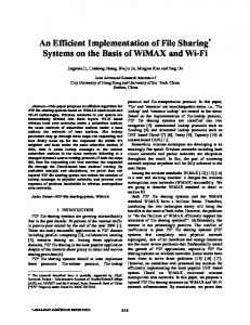
In lattice QCD the space-time is approximated by a four dimensional grid, the quarks are viewed as particles hopping between the grid sites and gluons are represented by parallel transporters that change the internal state of the quarks as they hop along the given link (see Fig. 1 for a schematic representation). The quark operator represents a discretization of the covariant derivative Dµ = ∂µ + igAµ , where Aµ is the color (gluon) field. The quark fields, ψn , are represented by 4 × 3 matrices at each lattice site and the gluon field Uµ (n) = eiagAµ (n) by SU (3) matrices. Wilson / = m + γµ Dµ is given by the discretization of m + D

U1 H6L

The structure of subnuclear particles like the proton and neutron is dictated by the dynamics of quarks and gluons. The strong force that binds them is described using quantum chromodynamics (QCD). Lattice QCD is a discretized version of this theory that makes it amenable to numerical simulations. The calculations involved are very demanding but they can be parallelized efficiently. Consequently, most lattice QCD simulations are run on traditional CPU clusters using fast interconnects. A recent alternative is to use graphics processing units (GPUs) for lattice QCD simulations [1], [2], [3], [4]. While difficult to program, these devices have very good floating point performance and very good memory bandwidth. For lattice QCD simulations, GPUs can outperform CPUs by large factors which allow us to build more compact and cost effective clusters. Currently most lattice QCD simulations run either in single GPU mode or on fat nodes with a few GPUs communicating over the PCI bus. This is the most efficient configuration if the memory requirements are relatively modest. However, this is not always feasible. Lattice QCD simulations can be performed using different discretizations of the QCD action depending on the problem studied. Traditional discretizations for the quark field introduce artifacts that are removed only in the continuum limit, i.e. when lattice spacing goes to zero. In particular, they break chiral symmetry which plays an important role for simulations close to the physical limit. Overlap discretization [5] of the quark field preserves this symmetry which allows us to capture the effects of chiral dynamics even at finite lattice spacing. Overlap formulation is numerically demanding and an efficient implementation requires significantly more memory

U1 H1L

I. I NTRODUCTION

U1 H10L

Keywords-Lattice QCD, GPU, overlap.

than traditional discretizations. To implement it on GPUs we need to be able to break the problem on multiple GPUs in order to satisfy the memory requirements. In this paper we present our implementation of the overlap operator in multiGPU context. The outline of the paper is the following. In Section II we review the numerical properties of the overlap operator. In Section III we discuss our parallelization strategy and the GPU-GPU communication structure. In Section IV we discuss the implementation of the dslash routine, which is the building block for the overlap operator. In Section V we discuss the implementation of the overlap operator, the required eigensolvers and conjugate gradient (CG) inverter used to compute the quark propagators.

U1 H5L

Abstract—Lattice QCD calculations were one of the first applications to show the potential of GPUs in the area of high performance computing. Our interest is to find ways to effectively use GPUs for lattice calculations using the overlap operator. The large memory footprint of these codes requires the use of multiple GPUs in parallel. In this paper we show the methods we used to implement this operator efficiently. We run our codes both on a GPU cluster and a CPU cluster with similar interconnects. We find that to match performance the CPU cluster requires 20-30 times more CPU cores than GPUs.

U1 H0L

arXiv:1106.4964v1 [hep-lat] 24 Jun 2011

Andrei Alexandru, Michael Lujan, Craig Pelissier, Ben Gamari, Frank Lee Department of Physics, The George Washington University 725 21st St. NW, Washington, DC 20052

ΨaΑ H3L U0 H3L

ΨaΑ H4L U0 H4L

Figure 1. Schematic representation of the lattice discretization: the quark a are associated with the sites of the lattice and the gauge variables fields ψα Uµ are defined on the links connecting the sites.

following matrix

1.0

±4 1 X Dw (m; U ) = (ma + 4)1 − Tµ (U ) , 2 µ=±1

∆

(1)

where Tµ are the parallel transporters for all 8 directions µ>0: µ cpu 2’:dslash bulk

3: cpu > cpu 4: cpu > gpu 5:scatter

stream 1

stream 2

Figure 5. Schematic diagram of the scheduling order for the multi-GPU dslash routine. The dashed lines represent CUDA synchronization points.

- a scatter routine that moves the data from the communication buffers to the appropriate sites and performs the required color multiplications, - communication routines that copy the GPU buffers from sender to receiver. The scatter/gather routines add very little overhead. Moving the data from one GPU to another is the most time consuming step. Fortunately, this step can be carried out in parallel with the bulk dslash calculation. As discussed in the previous section, the GPU to GPU communication occurs in three steps: GPU to CPU, CPU to CPU and CPU to GPU. The CPU to CPU transfer can be executed using a non-blocking MPI call. The CPU to GPU data transfer can be performed in parallel with the dslash kernel only if we use asynchronous CUDA copy instructions [12]. This only works if the CPU buffer involved uses pinned memory. Since the GPU kernels are issued asynchronously, we need to arrange carefully the execution order to ensure logical consistency. To achieve this we had to use CUDA streams: kernels attached to a particular stream are guaranteed to be executed in the order issued. Kernels, or asynchronous CUDA copy instructions, can be executed in parallel if they belong to different streams. The logical structure of the multi-GPU dslash routine is represented schematically in Fig. 5. Since gather, bulk dslash, and scatter kernels have to be executed sequentially, although they are attached to different streams, CUDA synchronization calls are used to enforce this constraint. A parallel code is efficient when the aggregate performance is proportional to the number of processes. We present here the results for strong scaling, i.e. performance of our codes for a lattice of fixed size that gets divided into smaller and smaller pieces as the number of processes is increased. Since the gather/scatter kernels take very little time, as long as the bulk dslash kernel takes more time than communication, the scaling will be almost perfect.

ææ

æ ç

æ

æ

æ

double precision performance model single precision

60 æ

40 æç ç æ

ç æ

ç æ

æ

ç æ

20

0

ç æ

0

5

10

15 20 GPU Count

25

30

Figure 6. Strong scaling for the multi-GPU dslash on a 243 ×64 lattice. The empty symbols represent the results of a performance model for the double precision routine and the solid points are measured on the GPU cluster described in the text.

However, as we increase the number of GPUs, the time for −1 the bulk dslash kernel will decrease as NGPU , whereas the −3/4 communication time will only decrease as NGPU . Eventually the communication time will dominate and scaling will suffer. The results presented here are measured on a GPU cluster with a single Tesla M2070 per node using QDR Infiniband network. On GPUs the error correction mode is turned on; this ensures the accuracy of the result at the expense of reducing the memory bandwidth. Since our kernels are memory bound their performance is also affected. The bandwidth measured in micro-benchmarks are 3.2 GB/s for the PCI bus and 4.2 GB/s for Infiniband. The gather/scatter kernels move 45/69 numbers per boundary site and their bandwidth performance is 55 GB/s. The double precision bulk dslash kernel performance is about 33 GFlops/s. Using these numbers we can construct a simple performance model for the multi-GPU routine. In Fig. 6 we present the performance of our codes and compare it with the predictions from the performance model. We see that for 32 GPUs our scaling efficiency is about 50% for a 243 × 64 lattice. For larger lattices the scaling is even better, for example for a 323 × 64 lattice the 32 GPUs scaling efficiency is about 60%. Our simple model follows closely the measured results for the double precision routine, but it overestimates slightly its performance. This is most likely due to the fact that, as in the case of the scalar product discussed in the previous section, the efficiency of the GPU kernels decreases as the size of the vectors gets smaller. To get a better picture, it is instructive to compare the performance of the GPU code with an equivalent code running purely on CPUs. The typical CPU dslash performance for double precision implementations is 1–2 GFlops/s [15]. Our own CPU implementation runs at 1.5 GFlops/s per core. This number was measured on a Cray XT-5 machine that uses very fast interconnects and dual hex-core AMD

Performance @GFLOPSD

Performance per GPU @GFLOPSD

80

æ

500 400

æ

300

æ æ

200 100 0

æ

æ æ æ ææ ææ æ æ

0

æ

CPU

æ

GPU

æ

10

20 30 40 GPU Equivalent Count

50

Figure 7. Strong scaling for the multi-GPU and multi-CPU dslash on a 243 × 64 lattice. The CPU-core count is rescaled by a factor of 22.

CPU per node. The CPUs run at 2.6 GHz. When comparing single-GPU performance it is then easy to see that the performance of one GPU is equivalent to 22 CPU cores. In the multi-GPU context it is less straightforward to define a measure, since scaling also plays an important role. To aid this comparison, we carried out a strong scaling study using our CPU dslash implementation running on the Cray machine. To compare the GPU and CPU performances we plot the aggregate performance of both CPU and GPU codes in Fig. 7: the CPU core count is translated into its GPU equivalent by dividing the total number of CPU cores by 22. This insures that the leftmost points in the graph overlap. If the CPU code scales similarly to the GPU code, the two curves should overlap. It is clear that the GPU codes scale better and that the equivalent CPU core count increases as we increase the number of GPUs. For example, the aggregate performance for 32 GPUs is 527 GFlops/s whereas the performance of 32×22 CPU-cores is only about 300 GFlops/s. V. OVERLAP OPERATOR IMPLEMENTATION Using the dslash and vector routines discussed in the previous sections we build now the overlap operator. To present the performance of our codes, we employ 243 × 64 lattices from one of our lattice QCD projects. The GPU cluster used for our testing has 32 GPUs with 3 GB of memory per GPU. The total GPU memory is then only sufficient to accommodate about 500 vectors. To compare the GPU performance with CPU codes, we run similar calculations on the Cray XT-5 machine described in the previous section. Since the scaling of the CPU codes is poorer than our GPU codes, we run our codes on 256 cores which is the minimum required to complete our tests in the time limit imposed by the scheduling system. Practical implementations for both polynomial and rational approximations require the calculation of the lowest lying eigenmodes of Hw . We also need to compute the

1200

0.12

1000 Polynomial Order

0.10

 Λ{¤

0.08 0.06 0.04 0.02

800 600 400 200

æ æ æ æ æ æ æ æ æ æ æ æ æ æ æ æ æ æ æ æ æ

æ æ æ æ æ æ æ æ æ æ æ æ æ æ æ æ æ æ æ æ æ æ æ æ æ æ æ æ æ æ æ æ æ æ æ æ æ æ æ æ æ æ æ æ æ æ æ æ æ æ æ æ æ æ æ æ æ æ æ æ æ æ æ æ æ æ æ æ æ æ æ æ æ æ æ æ æ æ æ æ æ æ æ æ æ æ æ æ æ æ æ æ æ æ æ æ æ æ æ æ æ æ æ æ æ æ æ æ æ æ æ æ æ æ æ æ æ æ æ æ æ æ æ æ æ æ æ æ æ æ æ æ æ æ æ æ æ æ æ æ æ æ æ æ æ æ æ æ æ æ æ æ æ æ æ æ æ æ æ æ æ æ æ æ æ æ æ æ æ æ æ æ æ æ æ æ æ æ æ æ æ æ æ æ æ æ æ æ æ æ æ æ æ æ æ æ æ æ æ æ æ æ æ æ æ æ æ æ æ æ æ æ æ æ æ æ æ æ æ æ æ æ æ æ æ æ æ æ æ æ æ æ æ æ æ æ æ æ æ æ æ æ æ æ æ

0.00 0

50 100 150 200 250 Number of Eigenvectors H{L

0

300

50

100 150 200 250 Number of Eigenvectors H{L

300

Figure 8. Eigenvalue magnitude for Hw as a function of eigenspace size. Each color represents a different 243 × 64 lattice.

Figure 9. Polynomial order required to approximate the sign function, sign(Hw ) with a precision δ = 10−9 in the subspace where |λ| > |λ` |.

eigenmodes of the overlap operator D to speed up propagator calculation. To compute these eigenmodes, we use implicitly restarted Arnoldi factorization [10], [11]. For a matrix A ∈ Cn×n , if we desire ` eigenmodes, we construct an Arnoldi factorization [16]:

order of the polynomial. Using the empirical formula [6]

AVk = Vk Hk + fk e†k

with (ek )n = δk,n ,

(10)

where Vk = {v1 , . . . , vk } ∈ Cn×k satisfies Vk† Vk = 1k , i.e. the n-dimensional vectors on the columns of Vk are orthonormal. The matrix Hk ∈ Ck×k is an upper Hessenberg matrix that is the restriction of A onto the Krylov space Kk (A, v1 ). The eigenvalues of Hk represent Ritz estimates of the eigenvalues of A and the residue, fk , can be used to gauge their accuracy. In practical calculations k  n. The implicitly restarted method uses a subspace of dimension k significantly larger than `, the desired number of eigenvectors. We set k = ` + ∆`, and at every step we remove from the k eigenmodes of Hk the ∆` undesired ones. The factorization is restarted using the new starting subspace and the whole process repeats until convergence. The optimal choice for our codes is ∆` ≈ 1.5` and then the number of vectors that need to be stored in memory is 2.5`. The first iteration in this algorithm requires k matrix multiplications and k(k − 1)/2 orthogonalizations. The subsequent iterations require only ∆` matrix-multiplications and k(k − 1)/2 − `(` − 1)/2 orthogonalizations. We now focus our discussion on the Hw eigensolver. The number of desired modes is dictated by both the structure of the low-lying spectrum of Hw and the available memory. In Fig. 8 we plot the magnitude |λ` | as a function of ` for a handful of lattices from our ensemble. It is clear that the spectral structure varies very little as we change the lattice. This can also be easily correlated with the performance of the overlap operator routine: the most expensive part is the sign multiplication routine, φ ← QP (Q2 )ψ, which for polynomial approximation is directly proportional to the

δ = Ae−bn

√



,

(11) √

with A = 0.41 and b = 2.1 and setting  = |λ` |/λmax we can compute the order of the polynomial required to achieve a precision of δ = 10−9 . The results are shown in Fig. 9. We see that going from ` = 100 to ` = 200 the polynomial order is reduced by about a factor of two. Since our GPU cluster can only store 500 vectors in device memory we set ` = 200 (recall that the Arnoldi eigensolver uses 2.5 × ` vectors). To accelerate the convergence of Hw eigenvectors we use Chebyshev acceleration [17]: we compute the eigenvectors of a polynomial Tn (Hw2 ) that has a more suitable eigenvalue structure but the same eigenvectors. We use a Chebyshev polynomial of the order 100 which speeds the convergence considerably (usually the Arnoldi eigensolver converges in one iteration). Our GPU cluster needs 0.27 hours to converge whereas the Cray machine needs 0.60 hours. Thus, one GPU is equivalent to 18 CPU cores for this code. Consumer level GPUs are significantly cheaper than the Tesla GPUs and offer similar performance for our codes. However, they have less memory available, usually 1.5–2 GB per GPU. We are forced then to use CPU memory to store the eigenvectors and the GPUs only to carry out the dslash multiplication. Due to the overhead associated with moving the vector over the PCI bus the effective performance of dslash is reduced by a factor of 5 to 10. In our case this problem is less severe because we use Chebyshev acceleration: computing T100 (Hw2 ) requires 200 dslash multiplications and the overhead is paid only once. Thus our effective dslash performance is very close to the pure GPU case. However, the orthogonalizations are computed on the CPU in this case and this adds a significant overhead. This mixed code takes 0.43 hours to converge on our GPU cluster, 60% more than the pure GPU code. This ratio depends on the number of eigenvectors requested, `, and

P (Q2 )ψ =

n X i=1

bi ψ, Q2 + ci

(12)

and compute (Q2 + ci )−1 ψ for all i’s at once using a multi-shifted CG method. The advantage of the polynomial approximation is that the memory requirements are small. Clenshaw recursion needs only 5 vectors whereas the multishifted CG needs 2n + 3 vectors. While the rational approximation converges very fast we still need n = 12–20. The double pass [18] variant of the rational approximation alleviates this problem at the cost of doubling the number of dslash matrix multiplications. In spite of this, the doublepass algorithm is faster than the single pass version [19] due to the reduced number of vector operations required. Moreover, it was found that the double-pass algorithm takes the same time irrespective of the order of the rational approximation. To decide on the optimal strategy, we compared the polynomial approximation with the double-pass algorithm and we run the codes on 8, 16, 24 and 32 GPUs. For this comparison we use ` = 40 to fit in the memory available in 8 GPU case. The double-pass algorithm used n = 18 and the exit criterion for CG was set to δ = 10−10 . The polynomial approximation was tuned to the same precision. The results of the test are presented in Fig. 10. It is clear that the polynomial approximation is the better choice and our codes are based on it. When we use all 200 eigenvectors the overlap multiplication routine requires 1.1 seconds on 32 GPUs whereas our Cray machine need 3.3 seconds. Thus, one GPU is equivalent to 24 CPU cores for this routine. We now turn our attention to the problem of computing the quark propagators. To use deflation, we have to compute the overlap eigensystem using the Arnoldi method. We first compute the eigenvectors of γ5 D in one chiral sector. Our γ-matrix basis is chiral and we can store the vectors that have definite chirality using only half the storage required for a regular vector. We can then store all ` = 200 Hw eigenvectors required for computing the overlap operator in device memory together with the 2.5×`0 = 250 half-vectors used by the Arnoldi algorithm. On our GPU cluster computing `0 = 100 eigenvectors to a precision of δ = 10−10

8 Time @sD

it will become worse as ` is increased. This is because the GPU time will increase linearly with ` since the GPUs are responsible for the dslash multiplications whereas the CPU time increases quadratically since the number of orthogonalizations required increases quadratically with `. We now turn our attention to the overlap operator D. As discussed in Section II, the sign function can be approximated using either a polynomial or a rational approximation. In the polynomial case, we expand the polynomials in terms of Chebyshev polynomials and use a Clenshaw recursion to evaluate P (Q2 )ψ. For the rational approximation we expand the rational function:

æ

æ

double pass

æ

polynomial

6 æ æ

4

æ

æ

æ æ

2 0 5

10

15

20 25 GPU Count

æ

30

Figure 10. Polynomial order required to approximate the sign function, sign(Hw ) with a precision δ = 10−9 in the subspace where |λ| > |λ` |.

takes 2.7 hours. On the Cray machine this takes 10.6 hours. Thus, one GPU is equivalent to 26 CPU cores for this code. On systems with reduced memory we can move the Arnoldi half-vectors on the CPU since they are accessed less frequently. In this case our GPU cluster requires 4.0 hours to converge which is 50% more than in the pure GPU case. We use an adaptive CG method [20] to compute D(m)−1 ψ with a precision of 10−8 . For a quark mass corresponding to mπ ≈ 200 MeV the adaptive method is 60% faster than the regular CG. To compute a full propagator for this mass the GPU cluster needs 0.52 hours and the Cray machine needs 2.3 hours. One GPU is then equivalent to 35 CPU cores for this code. Overall, a quark propagator calculation takes 3.5 hours on our 32 GPU cluster compared to 13.5 hours on the 256 cores Cray machine. This is consistent with the ratio of 22 CPU cores per one GPU that was computed for the dslash routine. VI. C ONCLUSIONS In this paper, we showed how to effectively employ GPUs for lattice QCD calculations using the overlap operator. The most challenging aspect of this calculation is the large amount of memory that needs to be accessed frequently. To deal with this issue, we had to implement our codes to run in parallel on multiple GPUs. Our optimization efforts focused on implementing the dslash routine efficiently. For 243 × 64 lattices our implementation scales reasonably well up to 32 GPUs where we still run at 50% efficiency. CPU clusters of comparable performance have worse scaling efficiency and the GPU/CPU core ratio for similar performance is even larger than 22, the ratio measured in the single-GPU case. To compute the overlap quark propagators we need to implement eigensolvers for both Hw and D. We used the implicitly restarted Arnoldi algorithm, and we found that the

performance is very similar to the dslash routine when all vectors reside in device memory. On systems where the device memory is not sufficient to hold all vectors, we found that storing the Arnoldi vectors in CPU memory is a reasonable alternative. The performance penalty is only 50–60%. We compared two different approximation strategies for the sign function used to define the overlap operator. We find that the polynomial approximation is better than the double-pass algorithm. Using this approximation the overlap operator runs at a rate equivalent to 24 CPU cores. In the future, we plan to investigate the single pass algorithm. The quark propagator is computed using an adaptive precision CG method which runs at a rate equivalent to 35 CPU cores. Overall, the GPU/CPU performance ratio for our codes is compatible with the ratio measured for the dslash routine. This result is not surprising since the most time consuming part of these codes is the dslash routine, but it takes careful planning to work around all possible bottlenecks. ACKNOWLEDGMENTS This work is partially supported by DOE grant DE-FG0295ER-40907. We wish to thank Mike Clark, Ron Babich and Balint Joo for useful discussions. The computational resources for this project were provided in part by the George Washington University IMPACT initiative. R EFERENCES [1] G. I. Egri et al., “Lattice QCD as a video game,” Comput. Phys. Commun., vol. 177, pp. 631–639, 2007. [2] M. A. Clark, R. Babich, K. Barros, R. C. Brower, and C. Rebbi, “Solving Lattice QCD systems of equations using mixed precision solvers on GPUs,” Comput. Phys. Commun., vol. 181, pp. 1517–1528, 2010. [3] R. Babich, M. A. Clark, and B. Joo, “Parallelizing the QUDA Library for Multi-GPU Calculations in Lattice Quantum Chromodynamics,” 2010. [4] A. Alexandru, C. Pelissier, B. Gamari, and F. Lee, “Multimass solvers for lattice QCD on GPUs,” 2011. [5] H. Neuberger, “Exactly massless quarks on the lattice,” Phys.Lett., vol. B417, pp. 141–144, 1998. [6] L. Giusti, C. Hoelbling, M. Luscher, and H. Wittig, “Numerical techniques for lattice QCD in the epsilon regime,” Comput.Phys.Commun., vol. 153, pp. 31–51, 2003. [7] T.-W. Chiu, T.-H. Hsieh, C.-H. Huang, and T.-R. Huang, “A note on the Zolotarev optimal rational approximation for the overlap Dirac operator,” Phys. Rev., vol. D66, p. 114502, 2002. [8] B. Jegerlehner, “Krylov space solvers for shifted linear systems,” unpublished, 1996. [Online]. Available: http: //arxiv.org/abs/hep-lat/9612014

[9] A. Li et al., “Overlap Valence on 2+1 Flavor Domain Wall Fermion Configurations with Deflation and Low-mode Substitution,” Phys.Rev., vol. D82, p. 114501, 2010. [10] D. C. Sorensen, “Implicit application of polynomial filters in a k-step Arnoldi method,” SIAM J. on Matrix Analysis and Applications, vol. 13, no. 1, pp. 357–385, 1992. [11] R. B. Lehoucq and D. C. Sorensen, “Deflation techniques for an implicitly restarted Arnoldi iteration,” SIAM J. Matrix Anal. Appl., vol. 17, no. 4, pp. 789–821, 1996. [Online]. Available: http://dx.doi.org/10.1137/S0895479895281484 [12] NVIDIA Corporation, “Cuda programming guide for cuda toolkit,” 2010. [Online]. Available: http://developer.nvidia. com/object/gpucomputing.html [13] MPI Forum, “MPI: A Message-Passing Interface Standard. Version 2.2,” September 4th 2009, available at: http://www. mpi-forum.org (Dec. 2009). [14] E. Gabriel, G. E. Fagg, G. Bosilca, T. Angskun, J. J. Dongarra, J. M. Squyres, V. Sahay, P. Kambadur, B. Barrett, A. Lumsdaine, R. H. Castain, D. J. Daniel, R. L. Graham, and T. S. Woodall, “Open MPI: Goals, concept, and design of a next generation MPI implementation,” in Proceedings, 11th European PVM/MPI Users’ Group Meeting, Budapest, Hungary, September 2004, pp. 97–104. [15] T. Wettig, “Performance of machines for lattice QCD simulations,” PoS, vol. LAT2005, p. 019, 2006. [16] W. E. Arnoldi, “The principle of minimized iteration in the solution of the matrix eigenvalue problem,” Quart. Appl. Math., vol. 9, pp. 17–29, 1951. [17] H. Neff, N. Eicker, T. Lippert, J. W. Negele, and K. Schilling, “On the low fermionic eigenmode dominance in QCD on the lattice,” Phys. Rev., vol. D64, p. 114509, 2001. [18] H. Neuberger, “Minimizing storage in implementations of the overlap lattice-Dirac operator,” Int. J. Mod. Phys., vol. C10, pp. 1051–1058, 1999. [19] T.-W. Chiu and T.-H. Hsieh, “A note on Neuberger’s double pass algorithm,” Phys. Rev., vol. E68, p. 066704, 2003. [20] N. Cundy et al., “Numerical methods for the QCD overlap operator. III: Nested iterations,” Comput. Phys. Commun., vol. 165, pp. 221–242, 2005.