Efficient Indexing Data Structures for Flash-Based Sensor ... - Cs.ucr.edu

Efficient Indexing Data Structures for Flash-Based Sensor Devices * SONG LIN University of California, Riverside and DEMETRIOS ZEINALIPOUR-YAZTI ** University of Cyprus and VANA KALOGERAKI, DIMITRIOS GUNOPULOS, WALID A. NAJJAR University of California, Riverside Flash Memory is the most prevalent storage medium found on modern Wireless Sensor Devices (WSDs). In this article we present two external memory index structures for the efficient retrieval of records stored on the local flash memory of a WSD. Our index structures, MicroHash and MicroGF (Micro Grid Files), exploit the asymmetric read/write and wear characteristics of flash memory in order to offer high performance indexing and searching capabilities in the presence of a low energy budget, which is typical for the devices under discussion. Both structures organize data and index pages on the flash media using a sorted by timestamp file organization. A key idea behind these index structures is that expensive random access deletions are completely eliminated. MicroHash enables equality searches by value in constant time and equality searches by timestamp in logarithmic time at a small cost of storing the index pages on the flash media. Similarly, MicroGF enables spatial equality and proximity searches in constant time. We have implemented these index structures in nesC, the programming language of the TinyOS operating system. Our trace-driven experimentation with several real datasets reveals that our index structures offer excellent search performance at a small cost of constructing and maintaining the index. Categories and Subject Descriptors: C.2.M [Computer-Communication Networks]: Miscellaneous; H.3.2 [Information Storage and Retrieval]: Information Storage; H.3.3 [Information Storage and Retrieval]: Information Search and Retrieval General Terms: Algorithms, Design, Experimentation Additional Key Words and Phrases: Wireless Sensor Networks, Flash Memory, Access Methods

* An earlier version of this paper appeared in [Zeinalipour-Yazti et al. 2005]. ** Corresponding Author: D. Zeinalipour-Yazti, [email protected], Tel: +357-22-892746, Fax: +357-22-892701, Address: 75 Kallipoleos Str., P.O. Box 20537, CY-1678, Nicosia, Cyprus. Authors’ addresses: S. Lin, Department of Computer Science & Engineering, University of California, Riverside, email: [email protected]; D. Zeinalipour-Yazti, Department of Computer Science, University of Cyprus, Cyprus, email: [email protected]; V. Kalogeraki, D. Gunopulos, W. Najjar, Department of Computer Science & Engineering, University of California, Riverside, email:{vana,dg,najjar}@cs.ucr.edu. Acknowledgements: This work was supported by grants from NSF ITR #0220148, #0330481. Permission to make digital/hard copy of all or part of this material without fee for personal or classroom use provided that the copies are not made or distributed for profit or commercial advantage, the ACM copyright/server notice, the title of the publication, and its date appear, and notice is given that copying is by permission of the ACM, Inc. To copy otherwise, to republish, to post on servers, or to redistribute to lists requires prior specific permission and/or a fee. c 20YY ACM 0362-5915/20YY/0300-0001 $5.00

ACM Transactions on Storage, Vol. V, No. N, Month 20YY, Pages 1–35.

2

·

S. Lin et al.

1. INTRODUCTION Rapid developments in wireless technologies and microelectronics have spawned a new generation of economically viable embedded sensor systems for monitoring and understanding the physical world [Warneke et al. 2001; Szewczyk et al. 2004; Intanagonwiwat et al. 2000; Sadler et al. 2004; Madden et al. 2002; Xu et al. 2004; Zeinalipour-Yazti et al. 2005]. Traditional sensing devices utilized over the years in meteorology, manufacturing and agriculture, are characterized by their passive mode of operation, their considerable size and the wired link that connects them to some centralized processing unit that enables storage and analysis. Wireless Sensor Devices (WSDs) on the other hand, are tiny computers on a chip that is often no bigger than a coin or credit card. These devices, equipped with a low frequency processor (≈4-58MHz) and a wireless radio, can sense parameters such as, light, sound, temperature, humidity, pressure, noise levels and movement at extremely high resolutions. This multitude of features constitute W SDs powerful devices which can be used for in-network processing, filtering and aggregation [Madden et al. 2003; 2002; Yao and Gehrke 2003]. The applications of sensor networks range from environmental monitoring (such as atmosphere and habitant monitoring [Szewczyk et al. 2004; Sadler et al. 2004]), to seismic and structural monitoring [Xu et al. 2004] and industry manufacturing (such as factory and process automation [Crossbow’05 ; Madden et al. 2002]). One of the key challenges in this new era of sensor networks, is the storage and retrieval of sensor data [Dai et al. 2004; Zeinalipour-Yazti et al. 2005; Ganesan et al. 2005]. Traditional techniques such as ([Madden et al. 2003; Deligiannakis et al. 2004; Intanagonwiwat et al. 2000]), work in a centralized way: the acquisition of data from the physical world is succeeded by the transmission of the respective data to the sink (querying node). The centralized repository, that contains the full resolution of sensor data, can then be utilized to resolve different types of queries. Such centralized data acquisition scenarios have a common problem of large energy consumption, as the whole universe of readings is transfered towards the sink, thus leading to a shorter sensor lifetime. In long-term deployments, it is often cheaper to keep a large window of measurements in-situ (at the generating site) [Zeinalipour-Yazti et al. 2005] and transmit the specific information to the sink only when requested. For example, biologists analyzing a forest are usually interested in the long-term behavior of the environment. Therefore the sensors are not required to transmit their readings to the sink at all times. Instead, the sensors can work unattended and store their reading locally until certain preconditions are met, or when the sensors receive a query over the radio that requests the respective data. Such in-network storage conserves energy from unnecessary radio transmissions, which can be used to increase the sampling frequency of the data and hence the fidelity of the measurements in reproducing the actual physical phenomena, and to prolong the lifetime of the sensing device. Currently, the deployment of the sensor technology is severely hampered by the lack of efficient infrastructure to store locally large amounts of sensor data measurements. The problem is that the local RAM memory of sensor nodes is both volatile and very limited (≈2KB-64KB). In addition, the non-volatile on-chip flash memory featured by most sensors is also very limited (≈32KB-512KB). However the limited ACM Transactions on Storage, Vol. V, No. N, Month 20YY.

Efficient Indexing Data Structures for Flash-Based Sensor Devices

·

3

local storage of sensor devices is expected to change soon. Several sensor devices, such as the RISE hardware platform [Neema et al. 2005; Banerjee et al. 2005], include off-chip flash memory which supplements each sensor with several megabytes of storage. Flash memory has a number of distinct characteristics compared to other storage media: Firstly, each page (typically 128B-512B) can only be written a limited number of times (≈10,000-100,000). Secondly, pages can only be written after they have been deleted in their entirety. Additionally, a page deletion always triggers the deletion of its respective block (≈8KB-64KB per block). Due to these fundamental constraints, efficient storage management becomes a challenging task. The problem that we investigate in this paper is how to efficiently organize the flash memory of a sensing device. Our desiderata are: (1) To provide efficient access to the data stored on flash by time or value, for both equality and range queries generated by the user. (2) To increase the longevity of the flash memory by spreading writes out uniformly so that the available storage capacity does not diminish at particular regions of the flash media. We present two new indexes, MicroHash and MicroGF, which serve as primitive structures for efficiently indexing temporal environmental and geographical data. Note that the data generated by sensor nodes has two unique characteristics: i) Records are generated at a given point in time (i.e. these are temporal records), and ii) The recorded readings are numeric values in a limited range. For example a temperature sensor might only record values between -40F to 250F with one decimal point precision, while the barometric pressure module used in the Mica Weather Board [Polastre 2003], measures pressure in the range 300mb to 1100mb, again with one decimal point precision [Polastre 2003]. Traditional indexing methods used in relational database systems [Fagin et al. 1979; Litwin 1980] are not suitable as these are mainly geared towards magnetic disks and do not take into account the asymmetric read/write behavior of flash media. Our indexing techniques have been designed for sensor nodes that feature large flash memories, such as the RISE [Neema et al. 2005] sensor, which provide them with several MBs of storage. MicroHash and MicroGF have been implemented in nesC [Gay et al. 2003] and use the TinyOS [Hill et al. 2000] operating system. This paper builds on our previous work in [Zeinalipour-Yazti et al. 2005], in which we presented the design and results of our MicroHash Index. In this paper we introduce several new improvements, such as an online compression algorithm and experimental evidence for efficient page read techniques. Additionally, we also develop an efficient solution to the problem of finding 2-D geographical information. Specifically, we present the design of the MicroGF index structure and experimentally demonstrate the advantages of such a structure against two popular alternatives: Grid Files and Quadtrees. Our contributions in this paper can be summarized as following: (1) We present the design and implementation of MicroHash, a novel index structure for supporting equality queries in environmental sensor nodes with limited processing capabilities and a low energy budget. ACM Transactions on Storage, Vol. V, No. N, Month 20YY.

4

·

S. Lin et al.

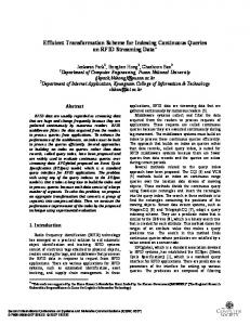
(2) We propose the design and implementation of MicroGF, a novel index structure for supporting spatial queries in sensor nodes equipped with GPS capabilities. (3) We present efficient algorithms for inserting, deleting and searching data records stored on flash media using our algorithms. (4) We describe the prototype implementation of MicroHash and MicroGF, and demonstrate the efficiency of our approach with an extensive experimental study using atmospheric readings from the University of Washington [ATMO’05 ], the Great Duck Island study [Szewczyk et al. 2004], and geographical readings from INFATI[Jensen et al. 2005]. The remainder of the paper is organized as follows: In Section 2 we present the memory hierarchy of a sensor node and a characterization of its performance characteristics using the RISE sensor. In Section 3 we formally define the indexing problem and then describe our data structures in Section 4. Section 5 and Section 6 describe the MicroHash index, search algorithms and search optimizations while Section 7 presents the MicroGF algorithm. Section 8 presents our experimental methodology and Section 9 the results of our evaluation. Finally we discuss related work in Section 10 and conclude the paper in Section 11. 2. THE MEMORY HIERARCHY In this section we briefly overview the architecture of a sensor node, with a special focus on its memory hierarchy. We also study the distinct characteristics of flash memory and address the challenges with regards to energy consumption and access time. 2.1 System Architecture The architecture of a sensor node (see Figure 1), consists of a microcontroller unit (MCU) which is interconnected to the radio, the sensors, a power source and the LEDs. The MCU includes a processor, a static RAM (SRAM) module and an on-chip flash memory. The processor runs at low frequencies (≈4-58MHz) which reduces power consumption. The SRAM is mainly used for code execution while in the latest generation of sensors, such as Yale’s 58MHz XYZ node [Lymberopoulos and Savvides 2005] and Intel’s 12MHz iMote (http://www.intel.com), it can also be used for in-memory (or SRAM) buffering. The choice of the right energy source is application specific. Most sensors either deploy a set of AA batteries or solar panels [Sadler et al. 2004]. Therefore a sensor node might have a very long lifetime. The on-chip flash provides a small non-volatile storage area (32KB-512KB) for storing the executable code or for accumulating values for a small window of time [Madden et al. 2003]. A larger external storage can also be supplemented to a sensor using the Serial Peripheral Interface (SPI) which is typically found on these devices. For example in the RISE platform, nodes feature a larger off-chip flash memory which provides the sensor with several GBs of storage. The external flash memory is connected to the MCU through a Serial Peripheral Interface (SPI), that operates at a fraction of the CPU frequency (e.g. cpuf8 req ). Therefore a faster processor would increase the maximum throughput of the SPI interface. Although it is currently not clear whether Moore’s Law will apply to the size and price of the sensor units or their hardware characteristics, we believe that ACM Transactions on Storage, Vol. V, No. N, Month 20YY.

Efficient Indexing Data Structures for Flash-Based Sensor Devices

·

5

MicroControllerUnit

Sensors

Processor ~4-58MHz

Power (AA, Solar)

Radio

SRAM ~8KB-64KB External Flash

SPI Bus 500KBps - 3MBps

Onchip Flash ~32KB-512KB LEDS

Fig. 1.

The Architecture of a typical Wireless Sensor.

future sensor nodes will feature more SRAM and flash storage, as more complex in-network processing applications, increase the memory and potentially the CPU demand. 2.2 Overview of Flash Memory Flash Memory is the most prevalent storage media used in current sensor systems because of its many advantages including: i) non-volatile storage, ii) simple cell architecture, which allows easy and economical production, iii) shock-resistance, iv) fast read access and power efficiency. These characteristics establish flash memory as an ideal storage media for mobile and wireless devices [Dipert and Levy 1994]. There are two different types of flash memory, NOR flash and NAND flash, which are named according to the logic gate of their respective storage cell. NAND flash is the newer generation of flash memory which is characterized by faster erase time, higher durability and higher density. NOR is an older type of flash which is mainly used for code storage (e.g. for the BIOS). Its main advantage is that it supports writes at a byte granularity as opposed to page granularity used in NAND flash. NOR flash has also faster access times (i.e. ≈200ns) than NAND (50-80µs) but lacks in all other characteristics such as density and power efficiency. For the rest of the paper we will focus on the characteristics of NAND memory as this is the type of memory used for the on-chip and off-chip flash of most sensors including the RISE platform. According to Micron (http://www.micron.com/), NAND memory is the fastest growing memory market in 2005 ($8.7 billion). Although reading from a NAND flash can be performed at any granularity, ranging from a single byte to a whole block (typically 8KB-64KB), it features a number of distinct constraints which can be summarized as following: (1) Delete-Constraint: Deleting data stored on flash memory can only be performed at a block granularity (i.e. 8KB-64KB). (2) Write-Constraint: Writing data can only be performed at a page granularity (typically 256B-512B), after the respective page (and its respective 8KB-64KB block) has been deleted. (3) Wear-Constraint: Each page can only be written a limited number of times ACM Transactions on Storage, Vol. V, No. N, Month 20YY.

6

·

S. Lin et al. NAND Flash installed on a Sensor Node Page Read Page Write Block Erase 1.17mA 37mA 57mA Time 6.25ms 6.25ms 2.26ms Data Rate 82KBps 82KBps 7MBps Energy 24µJ 763µJ 425µJ Flash Idle Flash Sleep 0.068mA 0.031mA Time N/A N/A Data Rate N/A N/A Energy 220µJ/sec 100µJ/sec

Table I. Performance Parameters for NAND Flash using a 3.3V voltage, 512B Page size and 16KB Block size

(typically 10,000-100,000). The design of our index structures in the remainder of this paper, considers the above constraints. 2.3 Access Time of NAND Flash Table I, presents the average measurements that we obtained from a series of microbenchmarks using the RISE platform along with a HP E3630A constant 3.3V power supply and a Fluke 112 RMS Multimeter. The first observation is that reading is three orders of magnitude less power demanding than writing. On the other hand, block erases are also quite expensive but can be performed much faster than the former two operations. Note that read and write operations involve the transfer of data between the MCU and the SPI bus, which becomes the bottleneck in the time to complete the operation. Specifically, reading and writing on flash media without the utilization of the SPI bus can be achieved in ≈50µ and ≈200µs respectively [Wu et al. 2003b]. Finally, our results are comparable to measurements reported for the MICA2 mote in [Dai et al. 2004] and the XYZ sensor in [Lymberopoulos and Savvides 2005]. Although these are hardware details, the application logic needs to be aware of these characteristics in order to minimize energy consumption and maximize performance. For example, the deletion of a 512B page will trigger the deletion of a 16KB block on the flash memory. Additionally the MCU has to re-write the rest unaffected 15.5KB. One of the objectives of our index design is to provide an abstraction which hides these hardware specific details from the application. 2.4 Energy Consumption of NAND Flash Another question is whether it is cheaper to write to flash memory rather than transmitting over the RF radio. We used the RISE mote to measure the cost of transmitting the data over a 9.6Kbps radio (at 60mA), and found that transmitting 512B (one page) takes on average 416ms or 82,368µJ. Comparing this with the 763µJ required for writing the same amount of data to local flash, along with the fact that transmission of one byte is roughly equivalent to executing 1120 CPU instructions, makes local storage and processing highly desirable. ACM Transactions on Storage, Vol. V, No. N, Month 20YY.

Efficient Indexing Data Structures for Flash-Based Sensor Devices

·

7

A final question we investigated is how many bytes we can store on local flash before a sensor runs out of energy. Note that this applies only to the case where the sensor runs on batteries. Double batteries (AA) used in many current designs operate at a 3V voltage and supply a current of 2500 mAh (milliAmp-hours). Assuming similarly to [Polastre 2003], that only 2200mAh is available and that all current is used for data logging, we can calculate that AA batteries offer 23, 760J (2200mAh * 60 * 60 * 3). With a 16KB block size and a 512B page size, we would have one block delete every 32 page writes (16KB/512B). Writing a page, according to our measurements, requires 763µJ while the cost of performing a block erase is 425µJ. Therefore writing 16KB of data requires: W rite16KB = (32pages ∗ 763µJ) + (425µJ) = 24, 841µJ

(1)

Using the result of the above equation, we can derive that by utilizing the 23, 760J offered by the batteries, we can write ≈15GB before running out of batteries ((23,760J * 16KB) / 24,841µJ). The interesting point is that even in the absence of a wear-leveling mechanism we would be able to accommodate the 15GB without exhausting the flash media. However this would not be true if we used solar panels [Sadler et al. 2004], which provide a virtually unlimited power source for each sensor device. Another reason why we want to extend the lifetime of the flash media is that the batteries of a sensor node could be replaced in cases where the devices remain accessible. 3. PROBLEM DEFINITION In this section we provide a formal definition of the indexing problems that the MicroHash and MicroGF structures address. We also describe how these cope with the distinct characteristics of flash memory. Let S denote some sensor that acquires readings from its environment every ǫ seconds (i.e. t = 0, ǫ, 2ǫ, ...). At each time instance t, the sensor S obtains a temporal data record drec = {t, v1 , v2 , ..., vx }, where t denotes the timestamp (key) on which the tuple was recorded, while vi (1 ≤ i ≤ x) represents the value of some reading (such as humidity, temperature, light, longitude and latitude, etc). Also let P = {p1 , p2 , ..., pn } denote a flash media with n available pages. A page canP store a finite number of bytes (denoted as psize ), which limits the capacity of P i n to i=0 psize . Pages are logically organized in b blocks {block1 , block2 , ..., blockb }, i each block containing n/b consecutive pages. We assume that pages are read on a page-at-a-time basis and that each page pi can only be deleted if its respective block (denoted as pblock ) is deleted as well (write/delete-constraint). Finally due i to the wear-constraint, each page can only be written a limited number of times (denoted as pwc i ). The MicroHash index supports efficient value-based equality queries and efficient time-based equality and range queries. These queries are defined as follows: Definition 3.1. Value-Based Equality Queries: a one dimensional query Q(vi , a) in which the field values of attribute vi are equivalent to value a. For example the query q=(temperature, 95F ) can be used to find time instances (ts) and other recorded readings when the temperature was 95F. ACM Transactions on Storage, Vol. V, No. N, Month 20YY.

8

·

S. Lin et al.

Definition 3.2. Time-Based Range and Equality Queries: a one dimensional query Q(t, a, b) in which the time attribute t, is between the lower and upper bound a and b respectively. The equality query is a special case of the range query Q(t, a, b) in which a = b. For example the query q=(ts, 100, 110) can be used to find the tuples recorded in the 10 second interval. The MicroGF index on the other hand, supports time-based equality and range queries, similarly to MicroHash. In addition, it supports efficient spatial queries defined as follows: Definition 3.3. Spatial Queries: a multi-dimensional query Q(v1 , v2 , ..., vx, Aquery ) in which the spatial attributes v1 , v2 ,...vx are in the query area Aquery . For example the query q=(x, y, cityN ewY ork) can be used to find all the positions appeared in New York city. Evaluating the above queries efficiently requires that the system maintains an index structure along with the generated data. Specifically, while a node senses data from its environment (i.e. data records), it also creates index entries that point to the respective data stored on the flash media. When a node needs to evaluate some query, it uses the index records to quickly locate the desired data. Since the number of index records might be potentially very large, these are stored on the external flash as well. Although maintaining index structures is a well studied problem in the database community [Fagin et al. 1979; Litwin 1980; Ramakrishnan and Gehrke 2002], the low energy budget of sensor nodes along with the unique read, write, delete and wear constraints of flash memory introduce many new challenges. In order to maximize efficiency our design objectives are as follows: (1) Wear-Leveling: Spread page writes out uniformly across the storage media P in order to avoid wearing out specific pages. (2) Block-Erase: Minimize the number of random-access deletions as the deletion of individual pages triggers the deletion of the whole respective block. (3) Fast-Initialization: Minimize the size of in-memory structures that will be required in order to use the index. 4. THE DATA STRUCTURES In this section we describe the data structures created in the fast but volatile SRAM to provide an efficient way to access data stored on the persistent but slower flash memory. First we describe the underlying organization of data on the flash media and then describe the involved in-memory data structures. 4.1 Flash Organization MicroHash and MicroGF use a Sorted-by-timestamp flash organization, in which records are stored on the flash media in a circular array fashion. This allows data records to be naturally sorted based on their timestamp and therefore our organization is Sorted by Timestamp. This organization requires the least overhead in SRAM (i.e. only one data write-out page). Additionally, as we will show in Section 5.4, this organization addresses directly the delete, write and wear constraint. When the flash media is full we simply delete the next block following ACM Transactions on Storage, Vol. V, No. N, Month 20YY.

Efficient Indexing Data Structures for Flash-Based Sensor Devices typedef struct Page { uint8_t typ:3; uint16_t crc:16; uint16_t pwc:15; uint8_t siz:7; uint32_t ppa:23; union { RootP rootP; DirP dirP; IdxP idxP; DataP dataP;}; } __attribute__((packed));

·

9

typedef struct IdxP { // optional anchor uint64_t lastTS; IdxRec records[IREC]; } __attribute__((packed)); typedef struct DataRec { timestamp_t ts; data_t val1; } __attribute__((packed)); typedef struct IdxRec { fladdress_t datap; // optional offset floffset_t offset; } __attribute__((packed));

typedef struct DataP { DataRec records[DREC]; } __attribute__((packed));

Fig. 2. Main data structures used in our nesC implementation. The example applies to the MicroHash Index while the MicroGF Index uses similar structures.

idx. Although other organizations in relational database systems, such as Sorted or Hashed on some attribute could also be used, they would have a prohibitive cost as the sensor would need to continuously update written pages (i.e. perform an expensive random page write). On the other hand, our Sorted-by-timestamp Organization always yields completely full data pages as data records are consecutively packed on the flash media. 4.2 In-Memory (SRAM) Data Structures The flash media is segmented into n pages, each with a size of 512B. Each page consists of a 8B header and a 504B payload. Specifically the header includes the following fields (also illustrated in Figure 2): i) A 3-bit Page Type (TYP) identifier. This identifier is used to differentiate between different types of pages such as data, index, directory and root pages. ii) A 16-bit Cyclic Redundancy Checking (CRC) polynomial on the payload, which can be used for integrity checking. When CRC is handled by lower levels then this field can be turned off. iii) A 7-bit Number of Records (SIZ), which identifies how many records are stored inside a page. Note that our implementation uses fixed size records that never span to more than one page. We chose such a scheme, as opposed to using variable length records, because records generated by a sensor always have the same size. To avoid segmentation, variable length records would require to keep a directory inside each page, which will keep track of the available space. iv) A 23-bit Previous Page Address (PPA), stores the address of some other page on the flash media giving in that way the capability to create linked lists on the flash. v) A 15-bit Page Write Counter (PWC), which keeps the number of times a particular page has been written to flash. While the header is identical for any type of page, the payload can store four different types of information: ACM Transactions on Storage, Vol. V, No. N, Month 20YY.

10

·

S. Lin et al.

SRAM p Write

Directory Page Index Page Data Page Empty Page

Flash Card

Fig. 3. Overview of the MicroHash Structure. While a node senses data from its environment it also creates index entries that point to the respective data stored on the flash media. When a node needs to evaluate some query, it uses the index records to quickly locate the desired data.

i) Root Page: contains information related to the state of the flash media. For example it contains the position of the last write (idx), the current cycle (cycle) and meta-information about the various indexes stored on the flash media. ii) Directory Page: contains a number of directory records (buckets) each of which contains the address of the last known index page mapped to this bucket. In order to form larger directories several directory pages might be chained using the 23-bit PPA address in the header. iii) Index Page: contains a fixed number of index records and the 8 byte timestamp of the last known data record. The latter field, denoted as anchor is exploited by timestamp searches which can make an informed decision on which page to follow next. Additionally, we evaluate two alternative index record layouts. The first, denoted as offset layout, maintains for each data record a respective pageid and offset, while the second layout, denoted as nooffset, maintains only the pageid of the respective data record. iv) Data Page: contains a fixed number of data records. For example when the record size is 16B then each page can contain 31 consecutively packed records. 5. INDEXING IN MICROHASH The MicroHash index is an efficient external-memory structure designed to support equality queries in sensor nodes that have limited main memory and processing capabilities. A MicroHash index structure consists of two modules (as shown in Figure 3): i) A Directory and ii) a set of Index Pages. The Directory consists of a set of buckets. Each bucket maintains the address of the newest (chronologically) index page that maps to that bucket. The Index Pages contain the addresses of the data records that map to the respective bucket. Note that there might be an arbitrarily large number of data and the index pages. Therefore these pages are stored on the flash media and fetched into main memory only when requested. The MicroHash index is built while data is being acquired from the environment and stored on the flash media. In order to better describe our algorithm we divide its operation in four conceptual phases: a) The Initialization Phase in which the root page and certain parts of the directory are loaded into SRAM, b) The Growing ACM Transactions on Storage, Vol. V, No. N, Month 20YY.

Efficient Indexing Data Structures for Flash-Based Sensor Devices

·

11

Phase in which data and index pages are sequentially inserted and organized on the flash media, c) The Repartition Phase in which the index directory is re-organized such that only the directory buckets with the highest hit ratio remain in memory, and the d) The Deletion Phase which is triggered for garbage collection purposes. 5.1 The Initialization Phase In the first phase the MicroHash index locates the root page on flash media. In our current design, the root page is written on a specific page on flash (page0). If page0 is worn out, we recursively use the next available page. Therefore a few blocks are pre-allocated at the beginning of the flash media for the storage of root pages. The root page indicates what types of indexes are available on the system and the addresses of their respective directories. Given that an application requires the utilization of an index I, the system pre-loads part of I ′ s directory into SRAM (detailed discussion follows in Section 5.3). The root and directory pages then remain in SRAM, for efficiency, and are periodically written out to flash. 5.2 The Growing Phase Let us assume that a sensor generates a temporal record drec = {t, v1 , v2 , ..., vx } every ǫ seconds, where t is the timestamp on which the record was generated and vi (1 ≤ i ≤ x) some distinct reading (e.g. humidity, temperature, etc). Instead of writing drec directly to flash, we use an in-memory (SRAM) buffer page pwrite (see Figure 4a). When pwrite gets full it is flushed to the address idx, where idx denotes the address after the last page write. Note that idx starts out as zero and this counter is incremented by one every time a page is written out. When idx becomes equal to the size of the flash media n, it is reset to zero. In order to provide a mechanism for finding the relative chronological order of pages written on the flash media, we also maintain the counter cycle, which is incremented by one every time idx is reset to zero. The combination of the provides the chronological order mechanism. Next we describe how index records are generated and stored on the flash media. The index records in our structure are generated whenever the pwrite buffer gets full. At this point we can safely determine the physical address of the records in pwrite (i.e. idx). We create one index record ir = [idx, of f set] for each data record in pwrite (∀drec ∈ pwrite ). For example assume that we insert the following 12 byte [timestamp, value] records into an empty MicroHash index: {[1000,50], [1001,52], [1002,52]}. This will trigger the creation of the following index records: { [0,0],[0,12],[0,24] }. Since pwrite is written to address idx the index records always reference data records that have a smaller identifier. The MicroHash Directory provides the start address of the index pages. It is constructed by providing the following three parameters: a) A lower bound (lb) on the indexed attribute, b) an upper bound (ub) on the indexed attribute and the number of available buckets c (note that we can only fit a certain number of directory buckets in memory). For example assume that we index temperature readings which are only collected in the following known and discrete range [−40..250], then we set lb = −40F , ub = 250F and c = 100. Initially each bucket represents exactly |lb..ub| c consecutive values although this equal splitting (which we call equiwidth splitting) ACM Transactions on Storage, Vol. V, No. N, Month 20YY.

12

·

S. Lin et al.

c. Deletion Phase

a. Growing Phase MicroHash

MicroHash

cycle=0 Flash Card

r = ts

v1

b1

b1 idx

v2

Directory [0-10]

cycle=1 Flash Card b0

b0 p write

idx

b2

Invalidation Threshold

b3



b2 b3

b. Repartition Phase

s=2 c=1

s=1 [10-20] c=3 s=0 [20-30] c=0

Directory s=2 c=1

s=0 [30-40] c=0

Index Pages

[0-10]

after

A:[10-15]

s=3 c=0

A1: [15-20]

s=4 c=1

s=0 [20-30] c=0

B: [30-40]

s=0 c=0

evicted to flash

Fig. 4. The three indexing phases: a) Growing Phase, b) Repartition Phase and c) Deletion Phase

is refined in the repartition phase based on the data values collected at run-time. 5.3 The Repartition Phase A drawback of the initial equiwidth bucket splitting approach is that some buckets may rarely be used while others may create long lists of index records. To overcome this problem, we use the following splitting policy: Whenever a directory bucket A links to more than τ records (user parameter), we evict to flash the bucket B, which was not used for the longest period of time (see Figure 4b). Note that this mechanism can be implemented using only two counters per bucket (one for the timestamp and one for the number of records). In addition to the eviction of page B, we also create a new bucket A1. Our objective is to provide a finer granularity to the entries in A as this bucket is the most congested one. Note that the values in A are not reassigned between A and A1 as it would happen in dynamic hashing techniques, such as extendible hashing [Fagin et al. 1979] or linear hashing [Litwin 1980]. The reason is that the index pages are on the flash media and updating these pages would result in a potentially very large number of random updates (which would be extremely expensive). Our equidepth, rather than equiwidth, bucket splitting approach keeps in memory finer intervals for index records used more frequently. Figure 4b shows that each bucket is associated with a counter s, that indicates the timestamp of the last time the buffer was used, and a counter c that indicates the number of index records added since the last split. In the example, the c = 3 value in bucket 2 (A:[10-20]) exceeds the τ = 2 threshold and therefore the index forces bucket 4 (B:[30-40]) to the flash media while bucket two is split into A:[10-15] and A1:[15-20]. Note that the A list now contains values in [10-20] while the A1 list ACM Transactions on Storage, Vol. V, No. N, Month 20YY.

Efficient Indexing Data Structures for Flash-Based Sensor Devices

·

13

contains only values in the range [15-20]. Although A currently stores records in the range [10-20], any future additions will only include values in the range [10-15]. The idea is that we don’t want to reassign the values of A, since these values reside on the flash media. In Section 6, we will show that this organization preserves efficient access to the data records. 5.4 The Deletion Phase In this phase the index performs a garbage collection operation of the flash media in order to make space for any newly acquired data. The phase is triggered after all n pages have been written to the flash media. This operation blindly deletes the next n/b pages, which is the whole block following the pointer idx (see Figure 4c). It is then triggered again whenever n/b pages have been written, where b is the number of blocks on the flash media. That leaves the index with n/b clean pages that can be used for future writes. Note that this might leave pointers from index pages referencing data that is already deleted. This problem is handled by our search algorithm described in the next section. The distinct characteristic of our garbage collection operation is that it satisfies directly the delete-constraint, because pages are deleted in blocks (which is cheaper than deleting a page-at-a-time). This makes it different from similar operations of flash file systems [Dai et al. 2004; Woodhouse ] that perform page-at-a-time deletions. Additionally, this mode provides the capability to ”blindly” delete the next block without the need to read or relocate any of the deleted data. The correctness of this operation is established by the fact that the index records always reference data records that have a smaller identifier. Therefore when an index page is deleted then we are sure that all associated data pages are already deleted. 6. SEARCHING IN MICROHASH In this section we show how records can efficiently be located by their value or timestamp. 6.1 Searching by Value The first problem we consider is how to perform value-based equality queries. Finding records by their value involves: a) locating the appropriate directory bucket, from which the system can extract the address of the last index page, b) reading the respective index pages on a page-by-page basis and c) reading the data records referred by the index pages on a page-by-page basis. Since SRAM is extremely limited on a sensor node we adopt a record-at-a-time query return mechanism, in which records are reported to the caller on record-by-record basis. This mode of operation requires three available pages in SRAM, one for the directory (dirP) and two for the reading pages (idxP,dataP), which only occupies 1.5KB. If more SRAM was available, the results could have been returned at other granularities as well. The complete search procedure is summarized in Algorithm 1. Note that the loadPage procedure in line 4 and 6 returns NULL if the fetched page is not in valid chronological order (with respect to its preceding page) or, if the fetched data records are not within the specified bucket range. We use these termination conditions, as the index records might point to deleted data pages. ACM Transactions on Storage, Vol. V, No. N, Month 20YY.

14

·

S. Lin et al.

Algorithm 1 EqualitySearch Input: value: the query (search predicate). Output: The records that contains value. 1: procedure EqualitySearch(value) 2: bucket = hash(value); 3: address = dirP [bucket].idxP ; 4: while ((idxP = loadPage(address)) != NULL) do 5: for i = 0 to |idxP.size| do 6: If ((dataP=loadPage(idxP[i].dataP))==NULL) 7: address=0; break; 8: If (dataP.record[idxP[i].offset]==value) 9: signal dataP.record[idxP[i].offset]; 10: end for 11: address = idxP.ppa; 12: end while 13: signal f inished; 14: end procedure

Recall that we do not update the index records during deletions for performance reasons. The validations applied by loadPage, ensure that we can safely terminate the search procedure. Finally, since the MicroHash index returns records on a record-at-a-time basis, we use a signal finished at the end to indicate that the search procedure has been completed. 6.2 Searching by Timestamp In this section we investigate time-based equality and range queries. First, note that if index pages were stored in a separate physical location, and thus not interleaved with data pages, the sorted (by timestamp) file organization would allow us to access any data record in O(1) time. However, this would also violate our wear leveling mechanism as we wouldn’t be able to spread out the page writes uniformly among data and index pages. Another approach would be to deploy an in-memory address translation table, such as the one used in [Wu et al. 2003b] and [Wu et al. 2003a], which would hide the details of wear-leveling mechanism. However, such a structure might be too big given the memory constraints of a sensor node and would also delay the sensor boot time. Efficient search can be supported by a number of different techniques. One popular technique is to perform a binary search over all pages stored on the flash media. This would allow us to search in O(log2 n) time, where n is the size of the media. For large values of n such a strategy is still expensive. For instance, with a 512MB flash media and a page size of 512B we would need approximately 20 page reads before we find the expected record. In our approach we investigate two binary search variants named: LBSearch and ScaleSearch. LBSearch starts out by setting a pessimistic lower bound on which page to examine next, and then recursively refines the lower bound until the requested page is found. ScaleSearch on the other hand exploits knowledge about the underlying distribution of data and index pages in order to offer a more aggressive search method that usually executes faster. ScaleSearch is superior to LBSearch when data and index pages are roughly uniformly distributed on the flash ACM Transactions on Storage, Vol. V, No. N, Month 20YY.

Efficient Indexing Data Structures for Flash-Based Sensor Devices lb

lb

lb t s LBSearch + Anchors

lb

lb tq

t q' shift t q''

te

lb t q' t q'' t q'''

te

t q'shift t q''

te

lb t q' t q'' t q'''

te

lb

scale t q shift

t s ScaleSearch + No Anchors

ts

15

lb t q shift

t s LBSearch + No Anchors

·

scale ScaleSearch + Anchors

lb tq

Fig. 5. Searching By Timestamp. ts : oldest timestamp on flash (te : newest), tq : the query (timestamp), lb: The lower bound obtained using either idxlb or idxscaled .

media but its performance deteriorates for skewed distributions. For the remainder of this section we assume that a sensor S maintains locally some indexed readings for the interval [ta ..tb ]. Also let x < y (and x > y) denote that the pair of x is smaller (and respectively greater) than the of y. When S is asked for a record with the timestamp tq , it follows one of the following approaches: i) LBSearch: S starts out by setting the lower bound : l m  tq −ts , if cycle == 0; ℜ l m idxlb (tq , ts ) t −t q s  idx + , otherwise ℜ

where idx is the address of the last written page and ℜ a constant indicating the maximum number of data records per page. It then deploys the LBSearch(ts, idxlb ) procedure as illustrated in Algorithm 2. It is easy to see that in each recursion step, LBSearch always moves clockwise (increasing time order) and that idxlb ≤ idxtq . Algorithm 2 LBSearch (No Anchors) Input: tq : the query (timestamp), current: begin search address Output: The page that contains tq . 1: procedure LBSearch(tq , current) 2: p = readP age(current); 3: if (isIndexP age(p)) then 4: // logical right shif t 5: return LBSearch(tq , current + 1); 6: else 7: t1 = P.record[0].ts; 8: t2 = P.record[P.lbu].ts; 9: if (t1 ≤ tq ≤ t2 ) then 10: return P ; 11: end if 12: return LBSearch(tq , current + idxlb (tq , t2 )); 13: end if 14: end procedure

ACM Transactions on Storage, Vol. V, No. N, Month 20YY.

16

·

S. Lin et al.

It is important to note that a lower bound can only be estimated if the fetched page, on each step of the recursion, contains a timestamp value. Our discussion so far, assumes that the only pages that carry a timestamp are data pages which contain a sequence of data records {[ts1 , val1 ]...[ts1 , valℜ ]}. In such a case, the LBSearch has to shift right until a data page is located. In our experiments we noted that this deficiency could add in some cases 3-4 additional page reads. In order to correct the problem we store the last known timestamp inside each index page (named Anchor). ii) ScaleSearch: When index pages are uniformly spread out across the flash media, then a more aggressive search strategy might be more effective. In ScaleSearch, which is the technique we deployed in MicroHash, instead of using idxlb in the first step we use idxscaled : l m  tq −ta ∗ idx , if cycle == 0; tb −tal m idxscaled (tq , ts ) t −t q a  idx + tb −ta ∗ n , otherwise.

We then use LBSearch in order to refine the search. Note that idxscaled might in fact be larger than idxtq in which case LBSearch might need to move counterclockwise (decreasing time order). Performing a range query by timestamp Q(tq , a, b) is a simple extension of the equality search. More specifically, we first perform a ScaleSearch for the upper bound b (i.e. Q(tq , b)) and then sequentially read backwards until a is found. Note that data pages are chained in reverse chronological order (i.e. each data page maintains the address of the previous data page) and therefore this operation is very simple. 6.3 Search Optimizations In this section we present three optimizations that increase the performance of the basic MicroHash approach. The first two methods alleviate the performance penalty that incurs because of index pages that are not fully occupied. Note that searching over partially full index pages, has as a result the unnecessary transfer of data between the MCU and the flash cells. The first method, named Elf-Like Chaining (ELC), eliminates non-full index pages, which as a result decreases the number of pages required to answer a query, and the second method, named TwoPhase Read minimizes the number of bytes transferred from the flash media. The third method attempts to minimize the amount of data that is read or written to the flash media. This is achieved by deploying some basic Run-Length Encoding compression scheme, while the sensor acquires the data.

6.3.1 Elf-Like Chaining (ELC). In the MicroHash index, pages are chained using a back-pointer as illustrated in Figure 6 (named MicroHash Chaining). Inspired from the update policy of the ELF filesystem [Dai et al. 2004], we also investigate, and later experimentally evaluate, the Elf-like Chaining (ELC) mechanism. The objective of ELC is to create a linked list in which each node, other than the last node, is completely full. This is achieved by copying the last non-full index page into a newer page, when new index records are requested to be added to the index. This procedure continues until an index page becomes full, at which point it is not ACM Transactions on Storage, Vol. V, No. N, Month 20YY.

·

Efficient Indexing Data Structures for Flash-Based Sensor Devices

17

further updated.

k

l

... pi

MicroHash Chaining

...

p i+3

copy

...

copy

...

k+l copy

pi

Elf-Like Chaining Fig. 6.

k

p i+3

Index Chaining Methods: a) MicroHash Chaining and b) ELF-like Chaining.

To better understand the two techniques, consider the following scenario (see Figure 6): An index page on flash (denoted as pi (i ≤ n)), contains k (k < psize ) index i records {ir1 , ir2 , ..., irk } that in our scenario map to directory bucket v. Suppose that we create a new data page on flash at position pi+1 . This triggers the creation of l additional index records, that in our scenario map to the same bucket v. In MicroHash Chaining (M HC), the buffer manager simply allocates a new index page for v and keeps the sequence {ir1 , ir2 , ..., irl } in memory until the LRU replacement policy forces the page to be written out. Assuming that the new index sequence is forced out of memory at pi+3 , then pi will be back-pointed by pi+3 as shown in Figure 6. In Elf-Like Chaining (ELC), the buffer manager reads pi in memory and then augments it with the l new index records (i.e. {ir1 , ..., irk , ..., irl+k }). However, pi is not updated due to the write and wear constraint, but instead the buffer manager writes the new l + k sequence to the end of the flash media (i.e. at pi+3 ). Note that pi is now not backpointed by any other page and will not be utilized until the block delete, guided by the idx pointer, erases it. The optimal compaction degree of index pages in ELC significantly improves the search performance of an index as it is not required to iterate over partially full index pages. However, in the worse case, ELC might introduce an additional page read per indexed data record. Additionally we observed in our experiments, presented in Section 9, that ELC requires on average 15% more space than the typical MicroHash chaining. In the worst case, the space requirement of ELC might double the requirement of M HC. k

...

k

copy

size-k pi

pi+2

Fig. 7.

k

copy

k

copy

size-k

size-k

...

pi+3

Sequential Trashing in ELC.

To understand the worst case scenario in ELC, consider again the scenario under discussion. This time assume that the buffer manager reads pi in memory and then augments psize (a full page) new index records as shown in Figure 7. That will evict i ACM Transactions on Storage, Vol. V, No. N, Month 20YY.

18

·

S. Lin et al.

Single vs Two Phase Page Read SRAM

Single versus Two Phase Page Read Phase I: Reads 8B Header, Phase II: Reads X Payload

SRAM

8

1 1,2

2 1

6

2

1

1

2

2

Flash Card

Flash Card

Time (ms)

1,2

Single Phase Two Phase

7

5 4 3 2 1 0 8

64

128

192

256

320

384

448

512

Bytes included in Page

Fig. 8. a) Illustration of the Single Phase and Two Phase Page Read strategies. b) Performance comparison of the strategies on the RISE platform.

pi to some new address (in our scenario pi+2 ). However some additional psize −k i records are still in the buffer. Assume that these pages are now evicted from main memory to some new flash position (in our scenario pi+3 ). So far we utilized three pages (pi , pi+2 and pi+3 ) while the index records could fit into only 2 index pages (i.e. k + psize records, k < psize ). When the same scenario is repeated, then we i i say that ELC suffers from Sequential Trashing and ELC will require double the required space to accommodate all index records. 6.3.2 Two-Phase Page Reads. Our discussion so far assumes that pages are read from the flash media on a page-by-page basis (usually 512B per page). When pages are not fully occupied, such as index pages, then many empty bytes (padding) is transferred from the flash media to memory. In order to alleviate this burden, we exploit the fact that reading from flash can be performed at any granularity (i.e. as small as a single byte). More specifically, we propose the deployment of a TwoPhase Page Read in which the MCU reads a fixed header from flash in the first phase, and then reads the exact amount of bytes in the next phase. The performance of two-phase reads versus single phase reads has been experimentally evaluated on the RISE platform [Neema et al. 2005] as is shown in Figure 8. Note that in order to initiate a read over the flash media there is a fixed 9-byte overhead for accessing the SPI bus. From our experimental analysis, it can be concluded that two-phase reading is almost always superior to its single phase counterpart, with an exception of pages which are adequately full (i.e. >90%). Minimizing the page reading time significantly minimizes energy consumption during searches. 6.3.3 Lossless Compression by Exploiting Temporal Locality. One common characteristic of real signals (or records) generated by sensing devices, is that consecutive time instances are correlated [Deligiannakis et al. 2004; Tang and Raghavendra 2004; Szewczyk et al. 2004]. For instance, a sensor device might generate the same temperature reading of 70F , for every second in the span of an hour. Therefore the ACM Transactions on Storage, Vol. V, No. N, Month 20YY.

Efficient Indexing Data Structures for Flash-Based Sensor Devices

·

19

temperature timeseries is characterized by temporal locality. In this subsection, we describe how a sensor device might exploit this additional parameter in order to perform some basic compression of the generated data values. Although one might argue that compression is of less importance, as flash storage can be very large and potentially very cheap, its importance originates from the fact that the predominant cost in the operation of a sensing device that records readings on local storage, comes from the bytes that are read or written to flash media. Therefore, we seek to reduce the amount of data stored on the flash media using some energy efficient compression algorithm that might significantly prolong the lifetime of the sensing device. Before outlining our solution, it is important to mention that any such technique, has to operate in a online fashion: the compression has to be performed before the data is stored on the flash media and while being generated by the sensing device. With this mode of operation the sensor can avoid the only other alternative which is the expensive offline compression method in which the data is compressed in a post-processing step. Finally, we seek to preserve the temporal order of data records, in order to keep the searching procedures outlined in section 6 unaffected. We propose the deployment of tools from the Information Theory field in order to address the online compression problem. Specifically, we utilize the Run-Length Encoding scheme in order to eliminate repetitive sequences that are a result of temporal locality. In Run-Length Encoding, consecutive values are replaced by a single value of the repeated value. For example the sequence {50,60,60,60,60,60,61,61} can be represented with {1:50,5:60,2:62}, where ”x : y” denotes that the value y is repeated for x consecutive time instances. In the example, this yields a saving of two integers. We examine how the encoding scheme can be applied in two different cases: i) Index Record Compression and ii) Data Record Compression. In the former case, which is illustrated in Figure 9b, we identify the correlated intervals and represent them using a single index record. Recall that the index records are generated as soon as the in-memory (SRAM) buffer page pwrite that contains the data records gets full. Therefore the correlated intervals are identified only within pwrite . In the example, we can see that each index record now stores the ranges [d2 , d5 ] and [d7 , d8 ] in which the temperature 60F was recorded, rather than one index record per data record (which is illustrated in Figure 9a). In the Data Record Compression case, which is illustrated in Figure 9c, we inverse the situation and record ranges of data values instead of ranges of index values. The compression is applied incrementally and directly on the data series which at this point resides in pwrite . Specifically, every time pwrite gets full, we execute in time O(k) the Run-Length Encoding technique on the k uncompressed data records of pwrite , where k ≤ n and n=|pwrite |. When k equals to zero, then this iterative procedure terminates, the respective index records are generated (using the typical microhash algorithm) and pwrite is written to flash. Although data record compression might be more storage efficient than index record compression, the former can only be applied on one-dimensional data records (i.e. (timestamp, val1 ) pairs). The N-dimensional case, where each data record has the following format: r=(timestamp, val1 , val2 , ..., valn ), turns out to be more complicated as the run-length encoding is designated to only run on a single ACM Transactions on Storage, Vol. V, No. N, Month 20YY.

·

20

S. Lin et al. MicroHash with Data Compression

MicroHash with Index Compression

MicroHash Index Page

Index Page

Index Page Index Records i2 i3

i1 d2

d3

i4

d4

Index Records i2 i3

i1

d5

d2,d5

Data Page

i4

d7,d8

i1

Index Records i2 i3

d2

d4

Data Page

Data Page

d1

d2

d3

d4

d5

d6

d7

d8

d1

d2

d3

d4

d5

d6

d7

d8

d1

59

60

60

60

60

61

60

60

59

60

60

60

60

61

60

60

59:1

Data Records

Data Records

Fig. 9.

i4

d2

d3

60:4 61:1

d4

d5

d6

d7

d8

60:2

Data Records

Exploiting Temporal Locality in order to compress MicroHash records .

correlated attribute rather than N attributes. Finally we mention that it would not be practical to apply any compression method directly on the binary sequence of records, as this prevents us from having direct access to each data record. For instance, suppose that we are given the following two sensor readings in their binary representation ([ts,val]): {[00000,00000], [00001,00000]}. Using run-length encoding we could have encoded this sequence using three numbers: {14, 1, 5} (14 consecutive ”0”, 1 consecutive ”1” and 5 consecutive ”0”). However such an encoding would not allow us to have direct access to the individual timestamps or values if the two data records, unless the data is first decoded.

7. INDEXING AND SEARCHING IN MICROGF In spatial query processing, the objective is to locate the data records which were recorded when the sensing device was within some predicate geographic region. For instance, a sensor device equipped with a GPS might provide the geographic coordinates of a moving zebra [Sadler et al. 2004] or car [Jensen et al. 2005]. A query might then be to locate the objects that were close to some predicate landmark. A naive method to cope with this kind of spatial queries, is to apply the MicroHash index directly on the two (or more) spatial dimensions. This would construct one index record for each respective spatial dimension. For example, data record < ts, x, y > can be indexed by keeping two different index records for x and y respectively. However, such an index structure is not very efficient, firstly due to the redundant space allocation, as we create multiple index records for each data record, and secondly because such a division can not efficiently capture the locality of spatial information for both equality and range queries. In this section we propose the MicroGF (Micro Grid File) index structure which is an external memory index structure designated for the efficient execution of spatial queries. The MicroGF index uses similarly to MicroHash, a set of directory and index pages to annotate where spatial data records are located on flash memory. The Directory consists of a set of buckets, which segments the recording space into multiple cells. Each bucket maintains the address of the newest (chronologically) index page that maps to the corresponding cell. The Index Pages contain the addresses of the data records that map to the respective bucket. ACM Transactions on Storage, Vol. V, No. N, Month 20YY.

Efficient Indexing Data Structures for Flash-Based Sensor Devices

·

21

7.1 MicroGF Index Data Structures Directory Page Data Structure: The directory of the MicroGF index structure consists of an N-dimensional grid of cells, where N denotes the number of spatial dimensions in the data records. To simplify discussion, we assume a 2-dimensional grid of cells in the xy-plane, that represents the coordinate space of some geographic area in which the sensing device generates spatial records. Therefore the MicroGF directory page consists of N*N square cells, each of which contains the address of the last known index page that mapped into this cell (geographic region). Index Page Data Structure: The Index Pages contain, similarly to MicroHash, the addresses of the respective data pages. In order to improve search performance each index record is divided into four equal-size quadrants. This essentially divides the recording space of a grid cell into four regions. Each quadrant then maintains the address for K records which map to the specific area. Algorithm 3 Insertion Input: MicroGF directory, data record < ts, x, y >. Output: updated MicroGF with < ts, x, y > inserted. 1: procedure Insert(ts, x, y) 2: Dir P = the directory entry that x, y resides in; 3: Idx P = Dir P.idx, Idx R = the first index record in Idx P ; 4: Q = f ind quadrant(Idx R, x, y); 5: if (Quadrant Insert(Q, x, y) == success) then signal finished; 6: else 7: Q.BID = f ind borrow quadrant(Q) 8: if (Quadrant Insert(Q.BID, x, y) == success) then signal finished; 9: else 10: if Idx P is not full then 11: Idx R′ = new index record, Q.SID = Idx R′ , 12: Q′ = f ind quadrant(Idx R′ , x, y), Quadrant Insert(Q′, x, y); 13: else 14: Idx P ′ = new index page, Idx P ′ → next = Idx P , 15: Dir P.idx = Idx P ′ , INSERT(ts, x, y); 16: end if 17: end if 18: end if 19: signal finished; 20: end procedure

7.2 Indexing in MicroGF The indexing procedure is triggered when the in-memory data record buffer pwrite , gets full. For each spatial record R we follow the following insertion algorithm (see Algorithm 3). First we locate the correct grid cell to which the data record R has to be assigned. This information is encapsulated in MicroGF’s directory. From there we extract the flash address of the newest (chronologically) index page (Idx P ) that maps to the corresponding cell. We then utilize the f ind quadrant(Idx R, x, y) function which identifies the quadrant Q, to which the data record R maps to. If this quadrant has enough ACM Transactions on Storage, Vol. V, No. N, Month 20YY.

22

1

·

S. Lin et al.

P3

P1

Borrow Bucket Index Page

00

1

01

10

11

00

01

10

11

2 3

1

P’1

P’3

4

0

P0

5

0

Next Record

P2

6

P’0

P’2 7

2

0

0

1

1

3 4

5 6

7

1

Fig. 10. Creation of a MicroGF Index Page. The two figures show at a high level how the trajectory on the left is encoded into a set of two index records.

space to accommodate R (i.e. if the number of indexed records is less than K), then the insertion is completed. Otherwise, the record R is assigned to adjacent quadrants having no records in it. These adjacent quadrants are named for convenience borrow quadrants. Note that borrow quadrants are allocated only within the same index record. If the number of records assigned to a cell does not fit into the adjacent borrow quadrants, then a new index record (Idx R′ ) is created. In this scenario, the original quadrant Q, is repartitioned into four sub-quadrants and the new index record is identified by a sub-region address (SID). To better understand the indexing process, assume that we have the trajectory shown in Figure 10 (left). The trajectory consists of seven data points, denoted with numbers 1 to 7. Also assume that the index record filling parameter K is set to 2. The first two records 1 and 2, are inserted into quadrants 01 and 00 separately (Figure 10 (right)). Record 3 and 4 are then both inserted into quadrant 10. As record 5 and 6 belong to quadrant 10 (but quadrant 10 is full), we check all 4 quadrants and find an empty quadrant 11, then we borrow the quadrant of 11 to index record 5 and 6 and update the BID of quadrant 10 as 11. When data record 7 comes, there is no space in either the mapping quadrant (10) or in the borrow quadrant (11). Therefore we create a new index record which accommodates the new record. Note that the borrow quadrant identifier (BID) of quadrant 10 is 11, which means we utilize 11 as the borrow quadrant to store the data records mapped into quadrant 10. In addition, the Sub-region Identifier (SID) of 10 in the first index record is 2, which means that there is no more space to index data record 7 in the first index record and we use the second index record to index it with smaller granularity. 7.3 Searching in MicroGF Searching in MicroGF is performed by first finding the directory cell Dir P , to which the query A belongs to. Then all the index pages that map to Dir P are searched. For each index page, we only have to check the quadrant Q that A ACM Transactions on Storage, Vol. V, No. N, Month 20YY.

Efficient Indexing Data Structures for Flash-Based Sensor Devices

·

23

Algorithm 4 Query Input: MicroGF directory, query area A. Output: data records < ts, P x, P y > within area A. 1: procedure Query(A) 2: Dir P = the directory entry that A overlaps; 3: Idx P = Dir P.idx; 4: while (Idx P != NULL) do 5: Q = f ind quadrant(Idx P, A); 6: while (Q != NULL) do 7: search(Q, A), search(Q.BID, A); 8: Q = Q.SID; 9: end while 10: Idx P = Idx P → next; 11: end while 12: signal finished; 13: end procedure

overlaps, the borrow quadrant of Q (Q.BID) and Q’s sub-region (Q.SID). The pseudocode of the MicroGF searching procedure is detailed in Algorithm 4. 7.4 The advantages of MicroGF Two other popular methods to index spatial records, are Grid Files [Nievergelt et al. 1984] and QuadTree [Samet 1984]. In Grid Files, a grid directory is utilized to partition the space into rectangle partitions and to index data page containing desired data records. However, the directory in Grid Files is very large and thus can not be maintained in SRAM as in MicroGF. In QuadTree, the recording space is recursively decomposed into quadrants. Each of the four quadrants becomes a node in the QuadTree. A larger quadrant is a node at a higher hierarchical level of the QuadTree, and smaller quadrants appear at lower levels. A problem with QuadTree, is the poor index space utilization for certain biased data distributions. For example, if all the data records are located under only one quadrant at each node, then only 25% of the index space is utilized. MicroGF, however, overcomes this problem by introducing the concept of borrow quadrants, which results in a better space utilization of index pages for any data set. With the more compact index pages, the query processing in MicroGF is faster and cheaper. These advantages of the MicroGF index structure are experimentally validated in Section 9.5. 8. EXPERIMENTAL METHODOLOGY In this section we describe the details of our experimental methodology. 8.1 Experimental Testbed We have implemented MicroHash along with a tiny LRU BufferManager in nesC [Gay et al. 2003], the programming language of TinyOS [Hill et al. 2000]. TinyOS is an open-source operating system designed for wireless embedded sensor nodes. It was initially developed at UC-Berkeley and has been deployed successfully on a wide range of sensors including our RISE mote. TinyOS uses a component-based architecture that enables programmers to wire together in on-demand basis the minimum required components. This minimizes the final code size and energy consumption ACM Transactions on Storage, Vol. V, No. N, Month 20YY.

24

·

S. Lin et al.

as sensor nodes are extremely power and memory limited. nesC [Gay et al. 2003] is the programming language of TinyOS and it realizes its structuring concepts and its execution model. Our implementation consists of approximately 5000 lines of code and requires at least 3KB in SRAM. Specifically we use one page as a write buffer, two pages for reading (i.e. one for an index page and one for a data page), one page as an indexing buffer, one for the directory and one final page for the root page. In order to increase insertion performance and index page compactness, we also supplement additional index buffers (i.e. 2.5KB-5KB). We had to write a library that simulates the flash media using an operating system file, in order to run our code in TOSSIM [Levis et al. 2003], the simulation environment of TinyOS. We additionally wrote a library that intercepts all messages communicated from TinyOS to the flash library and prints out various statistics and one final library that visualizes the flash media using bitmap representations. 8.2 PowerTOSSIM - Energy Modeling PowerTOSSIM is a power modeling extension to TOSSIM presented in [Shnayder et al. 2004]. In order to simulate the energy behavior of the RISE sensor we extended PowerTOSSIM and added annotations to the MicroHash structure that accurately provide information when the power states change in our environment. We have focused our attention on precisely capturing the flash performance characteristics as opposed to capturing the precise performance of other less frequently used modules (e.g. the radio stack). Our power model follows our detailed measurements of the RISE platform [Neema et al. 2005], which are summarized as following: We use a 14.8 MHz 8051 core operating at 3.3V with the following current consumption 14.8mA (On), 8.2mA (Idle), 0.2µA (Off). We utilize a 128MB flash media with a page size of 512B and a block size of 16KB. The current to read, write and block delete was 1.17mA, 37mA and 57µA and the time to read in the three pre-mentioned states was 6.25ms, 6.25ms, 2.27ms. Using these parameters, we performed an extensive empirical evaluation of our power model and found that PowerTOSSIM is indeed a very useful and quite accurate tool for modelling energy in a simulation environment. For example we measured the energy required to store 1 MB of raw data on an RISE mote and found that this operation requires 1526mJ while the same operation in our simulation environment returned 1459mJ, which has a error of only 5%. 8.3 Dataset Descriptions Since we cannot measure environmental conditions, such as temperature or humidity in a simulation environment, we adopt a trace-driven experimental methodology in which a real dataset is fed into the TOSSIM simulator. More specifically, we use the following datasets: Washington State Climate: This is a a real dataset of atmospheric data collected by the Department of Atmospheric Sciences at the University of Washington [ATMO’05 ]. Our 268MB dataset contains readings on a minute basis between January 2000 and February 2005. The readings, which are recorded at a weather logging station in Washington, include barometric pressure, wind speed, relative huACM Transactions on Storage, Vol. V, No. N, Month 20YY.

·

Efficient Indexing Data Structures for Flash-Based Sensor Devices

Temperature Histogram

Pressure Histogram

120000

200000 Pressure

100000

Number of Measurements

Number of Measurements

Temperature

80000 60000 40000 20000 0 -40

25

0 20 40 60 80 100 150 Temperature (Fahrenheit)

200

250

150000

100000

50000

0 900

950

1000 1050 Pressure (millibars)

1100

Fig. 11. Temperature (F) and Barometric Pressure (mb) readings recorded at an atmospheric monitoring site in Washington, USA. The last row indicates the respective distribution histograms for the two timeseries.

midity, cumulative rain and others. Since many of these readings are not typically measured by sensor nodes we only index the temperature and pressure readings, and use the rest readings as part of the data included in a record. Note that this is a realistic assumption, as sensor nodes may concurrently measure a number of different parameters. Figure 11 shows the timeseries for the readings used in our experiments along with the respective value distributions. Great Duck Island (GDI 2002): A real dataset from the habitat monitoring project on the Great Duck Island in Maine 1 . We use readings from one of the 32 nodes that were used in the Spring 2002 deployment, which included the following readings: light, temperature, thermopile, thermistor, humidity and voltage. Our dataset includes approximately 97,000 readings that were recorded between October and November 2002. INFATI: This is a real dataset derived from the INFATI Project [Jensen et al. 2005] carried out by Aalborg University. The readings are the GPS positions of 24 different cars moving in the city of Aalborg, Denmark in 2001. The readings include carid, timestamp, x-coordinate, y-coordinate, etc. Our dataset includes approximately 250,000 readings recorded between January and March 2001.

1 http://www.greatduckisland.net/

ACM Transactions on Storage, Vol. V, No. N, Month 20YY.

Space Overhead [Index/(Index+Data)] (%)

S. Lin et al. Index Space Overhead Ratio Varying Buffer Size and fixed 18B record size

45 Index on Temperature (Offset) Index on Temperature (noOffset) Index on Pressure (Offset) Index on Pressure (noOffset)

40 35 30 25 20 15 10 5 0 2.5

Fig. 12.

3

3.5 4 Buffer Size (KB)

4.5

5

Space Overhead [Index/(Index+Data)] (%)

·

26

Index Space Overhead Ratio Varying Record Size and fixed 3KB buffer Index on Temperature (Offset) Index on Temperature (noOffset) Index on Pressure (Offset) Index on Pressure (noOffset)

50 40 30 20 10 0 10

12 14 16 18 20 Record Size [8B/TS + 2B/attribute] (bytes)

22

Space Overhead of Index Pages with a) varying buffer size and b) varying record size.

9. EXPERIMENTAL EVALUATION In this section we present extensive experiments to demonstrate the performance effectiveness of the MicroHash Index structure. The experimental evaluation described in this section focuses on three parameters: i) Space Overhead, of maintaining the additional index pages, ii) Search Performance, which is defined as the average number of pages accessed for finding the required record and iii) Energy Consumption, for indexing the data records. Due to the design of the MicroHash and MicroGF index, each page is written exactly once during a cycle. Therefore there is no need to experimentally evaluate the wear-leveling performance. Finally we compare the performance of MicroGF with other spatial indexing techniques. 9.1 Overhead of Index Pages In the first series of experiments we investigate the overhead of maintaining the additional index pages on the flash media. For this reason we define the overhead ages ratio Φ as follows: Φ = DataPIndexP ages+IndexP ages . We investigate the parameter Φ using a) An increasing buffer size and b) An increasing data record size. We also evaluate two different index record layouts: a) Offset, in which an index record has the following form {pageid,offset} and NoOffset, in which an index record has the form {pageid}. We use the five year timeseries from the Washington state climate dataset and index data records based on their temperature and pressure attribute. The data record on each of the 2.9M time instances was 18 bytes (i.e. 8B timestamp + 5x2B readings). 9.1.1 Increasing Buffer Size. Figure 12 (left) presents our results using a varying buffer size. The figure shows that in all cases a larger buffer helps in fitting more index records per page which therefore also linearly reduces the overall space overhead. In both the pressure and temperature case, the noOffset index record layout significantly reduces the space overhead as less information is required to be stored inside an index record. The figure shows that indexing on pressure achieves a lower overhead. This is attributed to the fact that the pressure changes slower than the temperature over time. This leads to fewer evictions of index pages during the indexing phase which consequently also increases the index page occupancy. ACM Transactions on Storage, Vol. V, No. N, Month 20YY.

Efficient Indexing Data Structures for Flash-Based Sensor Devices

·

27

Index/Data Pages (left) — Grayscale Occupancy (right) 2.5K Buffer

Index/Data Pages (left) — Grayscale Occupancy (right) 10K Buffer

Fig. 13. Bitmap Illustrations of the Flash Media. Each pixel represents a page on flash media. The left column shows the index pages (in black) and the data pages (in white). The right column uses a 256-bit grayscale image to color the fullness of index pages (black=empty).

We found that a 3KB buffer suffices to achieve an occupancy of 75-80% in index pages. This can be viewed in the bitmap illustrations of the flash media in Figure 13. The figures show two characteristics: a) The number of index page on flash and b) the occupancy of these pages using a 256-bit grayscale pixel (where black denotes an empty page). As we can see, providing a larger buffer during the indexing phase not only decreases the number of index pages (i.e. less black pixels) on flash but also makes these index pages higher occupied (i.e. less darker pixels). 9.1.2 Increasing Data Record Size. Sensor nodes usually deploy a wide array of sensors, such as a photo sensor, magnetometer, accelerometer and others. Therefore the data record size on each time instance, might be larger than the minimum 10B size (8B timestamp and 2B data value). Figure 12 (right) presents our results using a varying data record size. The figure shows that in all cases a larger data record size decreases the space overhead proportion. Therefore it does not become more expensive to store the larger data records on flash. 9.2 Searching By Timestamp In the next experimental series, we investigate the average number of pages that must be read in order to find a record by its timestamp. Note that if we did not use an index, and thus had only data records on the flash, then we could ACM Transactions on Storage, Vol. V, No. N, Month 20YY.

·

28

S. Lin et al.

Search By Timestamp Performance (Index on Temperature)

Search By Timestamp Performance (Index on Pressure) 5.5

LBSearch + NoAnchor LBSearch + Anchor ScaleSearch + NoAnchor ScaleSearch + Anchor

10

Pages Read (Page Size 512B)

Pages Read (Page Size 512B)

11

9 8 7 6 5 4

LBSearch + NoAnchor LBSearch + Anchor ScaleSearch + NoAnchor ScaleSearch + Anchor

5

4.5

4

3.5

3 2.5

3

Fig. 14.

3.5 4 Buffer Size (KB)

4.5

5

2.5

3

3.5 4 Buffer Size (KB)

4.5

5

Search-By-Timestamp Performance of the MicroHash Index.

find the expected record in O(1) time as we could manipulate the position of the record directly. However, this would also violate our wear leveling mechanism as we wouldn’t be able to spread out the page writes evenly among data and index pages. We evaluate the proposed search by timestamp methods LBSearch and ScaleSearch under two different index page layouts: a) Anchor, in which every index page stores the last known data record timestamp and b) NoAnchor, in which an index page does not contain any timestamp information. Figure 14 shows our results using the Washington state climate dataset for both an index on Temperature (left) and an Index on Pressure (right). The figure shows that using an anchor inside an index pages is a good choice as it usually reduces the number of page reads by two, while it does not present a significant space overhead (only 8 additional bytes). The figure also shows that ScaleSearch is superior to LBSearch as it exploits the uniform distribution of index pages on the flash media. This allows ScaleSearch to get closer to the result, in the first step of the algorithm. The figure finally shows that even though the time window of the query is quite large (i.e. 5 years or 128MB), ScaleSearch is able to find a record by its timestamp in approximately 3.5-5 page reads. Given that a page read takes 6.25ms, this operation requires according to the RISE model only 22-32ms or 84-120µJ. 9.3 Searching by Value: MicroHash vs ELF-Like Chaining The cost of searching a particular value on the flash media is linear with respect to the size of the flash media. However, a simple linear scan over 256 thousands pages found on a 128MB flash media, would result in an overwhelming large search cost. One factor that significantly affects search performance, is the occupancy of index pages. In the basic MicroHash approach, index pages on the flash might not be fully occupied. If index pages are not fully utilized, then a search requires to iterate over more pages than necessary. In this section we perform an experimental comparison of the index chaining strategies presented in Section 6.3. We evaluate both MicroHash Chaining (MHC) and Elf-like chaining (ELC) using a fixed 3KB buffer. We deploy the chaining methods when the temperature is utilized as the index (we obtained similar results ACM Transactions on Storage, Vol. V, No. N, Month 20YY.

Efficient Indexing Data Structures for Flash-Based Sensor Devices Insertion Performance: ELC vs MHC Chaining Histogram

·

29

Search Performance: ELC vs MHC Chaining Histogram

5000

Pages

Number of Page Reads (Data+Index)

MHC Writes ELC Writes ELC Total (Read+Write)

4000

3000

2000

1000

0

MHC Index Read MHC Total Read ELC Index Read ELC Total Read

10000 8000 6000 4000 2000 0

20

40

60 Temperature

80

100

20

40

60 Temperature

80

100

Fig. 15. Comparing MicroHash Chaining (MHC) with ELF-like Chaining (ELC) using a) Insertion Performance and b) Searching Performance by Value.

for pressure). Our evaluation parameters are : a) Indexing Performance (pages written) and b) Search Performance (pages read). Figure 15 (left) shows that MHC always requires less page writes than ELC. The reason is that ELC’s strategy results in about 15% sequential trashing, which is the characteristic presented in Section 6.3. Additionally, ELC requires a large number of page reads in order to replicate some of the index records. This is presented in the ELC Total plot, which essentially shows that it requires as many page reads as page writes in order to index all records. On the other hand, ELC’s strategy results in linked lists of fully occupied index pages than MHC. This has as a result, an improved search performance since the system is required to fetch less index pages during search. This can be observed in Figure 15 (right), in which we present the number of index pages read and the total number of pages (index + data). On the other hand, we also observe that ELC only reduces the overall read gain to about 10%. This happens because the reading of data pages, dominates the overall reading cost. However when searches are more frequent, then the 10% is still an advantage and therefore ELC is more appropriate than its counterpart MHC. 9.4 Great Duck Island Trace We index measurements from the great duck island study, described in Section 8.3. For this study we allocate a fixed 3KB index buffer along with a 4MB flash media that has adequate space to store all the 97,000 20-byte data readings. In each run, we index on a specific attribute (i.e. Light, Temperature, Thermopile, Thermistor, Humidity and Voltage). We then record the overhead ratio of index pages Φ, the energy required by the flash media to construct the index as well as the average number of page reads that were required to find a record by its timestamp. We omit the search by value results since these are very similar to those presented in the previous subsection. Table II shows that the index pages never require more that 30% more space on the flash media. For some readings that do not change frequently (e.g. humidity), we observe that the overhead is as low as 8%. The table also shows that indexing the records has only a small increase in energy demand. Specifically, the energy cost ACM Transactions on Storage, Vol. V, No. N, Month 20YY.

30

·

S. Lin et al. Index On Attribute Light Temperature Thermopile Thermistor Humidity Voltage

Overhead Ratio Φ(%) 26.47 27.14 24.08 14.43 7.604 20.27

Energy Index (mJ) 4,134 4,172 4,005 3,554 3,292 3,771

ScaleSearch Avg Page Read 4.45 5.45 6.29 5.10 2.97 4.21

Table II. Performance Results from Indexing and Searching the Great Duck Island dataset.

of storing the records on flash without an index was 3042mJ, which is on average only 779mJ less than using an index. Therefore maintaining the index records does not impose a large energy overhead. Finally the table shows that we were able to find any record by its timestamp with 4.75 page reads on average.

Grid Files QuadTree

2000

MicroGF

1000

500

1 2 3 4 Dataset(1,2. Synthesis Datasets; 3. INFATI; 4. Weather Data)

Index Space Overhead Ratio Space Overhead [(Index/(Index+Data)](%)

Average Page Reads (Data+Index)

Search Performance: MicroGF vs Grid Files and QuadTree 3000

40 Grid Files QuadTree MicroGF 20

10

5 1

2 3 4 Dataset(1,2. Synthesis Datasets; 3. INFATI; 4. Weather Data)

Fig. 16. Comparing MicroGF with Grid Files and QuadTree using a)Searching Performance by Value. b)Space overhead of Index pages.

9.5 MicroGF vs Grid File and QuadTree In this section we compare the performance of the MicroGF structure with two hash-based spatial indexing techniques: Grid Files and QuadTree. We utilize four datasets: 2 synthetic data sets with 250K random points in a two dimensional space, the INFATI data set [Jensen et al. 2005] and the weather data set [ATMO’05 ]. We segment the recording space into 36 subregions and generate a random query area for each subregion. We then compare the average page access number for a query ages and the space overhead of index pages (Φ = DataPIndexP ages+IndexP ages ). As is shown in Figure 16, on average the MicroGF algorithm accesses 40% less pages than QuadTree and 80% less pages than Grid Files in query processing. In addition, the index space overhead of MicroGF is 15% less than QuadTree and 56% less than Grid Files. This is mainly attributed to the following two reasons: a) Borrow Quadrants can utilize the index page space more efficiently and b) Subregion segmentation adjusts the index structure dynamically according to the distribution of data. ACM Transactions on Storage, Vol. V, No. N, Month 20YY.

Efficient Indexing Data Structures for Flash-Based Sensor Devices

·

31

10. RELATED WORK In this section, we review prior work on storage and indexing techniques for sensor networks. While our work addresses both problems jointly, most prior work has considered them in isolation. A large number of flash-based file systems have been proposed in the last few years, including the Linux compatible Journaling Flash File System (JFFS and JFFS2) [Woodhouse ], the Yet Another Flash File System (YAFFS) [Wookey ] specifically designed for NAND flash with it being portable under Linux, uClinux, and Windows CE. Wear-Leveling techniques on flash memory have been reported by flash card vendors such as Sandisk [Sandisk ]. These techniques are executed by a microcontroller which is located inside the flash card. The Wear-Leveling techniques are only executed within 4MB zones and are thus local rather than global which is the case in MicroHash and MicroGF. A main drawback of the local wear-leveling techniques is that the writes are no longer spread out uniformly across all available pages. Finally these techniques assume a dedicated controller while our techniques can be executed by ordinary microcontroller of the sensor device. Other vendors might utilize their own proprietary wear-leveling techniques. However, it is difficult to compare our structure with these techniques because most vendors usually don’t disclose any details with regards to their architecture or algorithms. Recently various techniques have been proposed for data storage and indexing in sensor networks. Matchbox is a simple file system packaged with the TinyOS distribution [Hill et al. 2000]. It hides the lower details of wear-leveling and provides a pointer to each file (page in our context) on the flash memory. Had we used such an approach, would require a very large footprint to keep track of these pointers. The Efficient Log Structured Flash File System (ELF) [Dai et al. 2004] is a log-like file structure designed for wear-leveling. It works by updating desired file page and writing it into a new flash memory space. A few other indexing schemes have been proposed in the context of sensor networks. One such scheme is T SAR in [Desnoyers et al. 2005], which stores data locally at sensor nodes and index them by higher tier nodes called proxies. Distributed Index of Features in Sensor networks (DIFS [Greenstein et al. 2003]) and Multi-dimensional Range Queries in Sensor Networks (DIM [Li et al. 2003]) extend the data-centric storage approach to provide spatially distributed hierarchies of indexes to data. All these techniques provide index topologies at the network level, but do not provide details on how to efficiently write the index information into the sensor flash memories as we do in our approach. An R-Tree index structure for flash memory on portable devices, such as PDAs and cell phones, has been proposed in [Wu et al. 2003b]. These structures provide an efficient algorithm to compact several consecutive index units (R-tree nodes) into a page for better space utilization and search. In addition, they use an in-memory address translation table, which hides the details of wear-leveling mechanism. However, such a structure has a very large footprint (3-4MB) which constitute it inapplicable for all sensor nodes (2KB-64KB RAM) we have so far. Other hash-based techniques (like Z-ordering and grid files) have been proposed for spatial data indexing. Z-ordering [Orenstein and Merrett 1984] divides each attribute into equal ACM Transactions on Storage, Vol. V, No. N, Month 20YY.

32

·

S. Lin et al.

segments and impose a linear ordering on the domain. The position in high dimensional space is therefore mapped to a one dimensional array. A problem with Z-ordering is that not all the points close in X-Y plane is close in Z-value. Another problem is that the bucket boundary of Z-ordering is fixed at the very beginning which makes it inefficient on non-uniformly distributed data. Grid file [Nievergelt et al. 1984] is another kind of hash-based spatial index structure. The grid file partitions the space into rectangle partitions and utilizes grip directory (a matrix) to link to the data page containing a desired point. The size of the grid directory is adjusted as in extendible hashing. Several variants of grid files have been proposed [Seeger and Kriegel 1990; Whang and Krishnamurthy 1985] to improve the performance of grid files for biased distributed data. However, these algorithms read flash data records multiple times due to bucket update, which is inefficient in our context. As has been shown in our paper, the MicroGF algorithm is robust on biased distributed data while overcoming the small RAM and wear-leveling problems. Systems such as TinyDB [Madden et al. 2003] and Cougar [Yao and Gehrke 2003] achieve energy reduction by pushing aggregation and selections in the network rather than processing everything at the sink. Both approaches propose a declarative approach for querying sensor networks. These systems are optimized for sensor nodes with limited storage and relatively short-epochs, while our techniques are designated for sensors with larger external flash memories and longer epochs. Note that in TinyDB users are allowed to define fixed size materialization points through the STORAGE POINT clause. This allows each sensor to gather locally in a buffer some readings, which cannot be utilized until the materialization point is created in its entirety. Therefore even if there was enough storage to store MBs of data, the absence of efficient access methods makes the retrieval of the desired values quite expensive. In Data Centric Routing (DCR), such as directed diffusion [Intanagonwiwat et al. 2000], low-latency paths are established between the sink and the sensors. Such an approach is supplementary to our framework. In Data Centric Storage (DCS) [Shenker et al. 2003] data with the same name (e.g. humidity readings) is stored at the same node in the network, offering therefore efficient location and retrieval. However the overhead of relocating the data in the network will become huge if the network generates many MBs of GBs of data. Finally, local signal-based compression techniques, such as the one proposed in [Deligiannakis et al. 2004], could improve the compression efficiency of our framework and their investigation will be a topic of future research. 11. CONCLUSIONS In this paper we propose Microhash and MicroGF which are efficient external memory hash index structures that address the distinct characteristics of flash memory. We also provide an extensive study of NAND flash memory when this is used as a storage media of a sensor node and validate various design principles using our RISE platform. We expect that our proposed access method will provide a powerful new framework to cope with new types of queries, such as temporal or top-k [Zeinalipour-Yazti et al. 2005], that have not been addressed adequately to ACM Transactions on Storage, Vol. V, No. N, Month 20YY.

Efficient Indexing Data Structures for Flash-Based Sensor Devices

·

33

this date. Our experimental testbed written in nesC with real traces from environmental and habitant monitoring shows that the structures we propose are both efficient and practical. REFERENCES ATMO’05. Live From Earth and Mars Project. University of Washington, Seattle http://wwwk12.atmos.washington.edu/k12/grayskies/. Banerjee, A., Mitra, A., Najjar, W., Zeinalipour-Yazti, D., Kalogeraki, V., and Gunopulos, D. 2005. Rise co-s : High performance sensor storage and co-processing architecture. In Second Annual IEEE Communications Society Conference on Sensor and Ad Hoc Communications and Networks. Crossbow’05. Crossbow Technology Inc. http://www.xbow.com/. Dai, H., Neufeld, M., and Han, R. 2004. Elf: an efficient log-structured flash file system for micro sensor nodes. In Proceedings of the 2nd international conference on Embedded networked sensor systems. 176–187. Deligiannakis, A., Kotidis, Y., and Roussopoulos, N. 2004. Compressing historical information in sensor networks. In Proceedings of the ACM SIGMOD international conference on Management of Data. 527–538. Desnoyers, P., Ganesan, D., and Shenoy, P. 2005. Tsar: A two tier sensor storage architecture using interval skip graphs. In Proceedings of the 3rd international conference on Embedded networked sensor systems. 39–50. Dipert, B. and Levy, M. 1994. Designing with Flash Memory. Fagin, R., Nievergelt, J., Pippenger, N., and Strong, H. 1979. Extendible hashing - a fast access method for dynamic files. ACM Transactions on Database System 4, 3, 315–344. Ganesan, D., Greenstein, B., Perelyubskiy, D., Estrin, D., and Heidemann, J. 2005. Multiresolution storage and search in sensor networks. ACM Transactions on Storage 1, 3, 277–315. Gay, D., Levis, P., Von, B., Welsh, M., Brewer, E., and Culler, D. 2003. The nesc language: A holistic approach to networked embedded systems. In ACM SIGPLAN Conference on Programming Language Design and Implementation. Greenstein, B., Estrin, D., Govindan, R., Ratnasamy, S., and Shenker, S. 2003. Difs: A distributed index for features in sensor networks. In First IEEE Ineternational Workshop on Sensor Network Protocols and Applications. Hill, J., Szewczyk, R., Woo, A., Hollar, S., Culler, D., and Pister, K. 2000. System architecture directions for networked sensors. SIGPLAN NOTICE 35, 11, 93–104. Intanagonwiwat, C., Govindan, R., and Estrin, D. 2000. Directed diffusion: A scalable and robust communication paradigm for sensor networks. In Mobile Computing and Networking. 56–67. Jensen, C., Lahrmann, H., Pakalnis, S., and Runge, J. 2005. The infati data. Levis, P., Lee, N., Welsh, M., and Culler, D. 2003. Tossim: Accurate and scalable simulation of entire tinyos applications. In Proceedings of the First ACM Conference on Embedded Networked Sensor Systems. Li, X., Kim, Y., Govindan, R., and Hong, W. 2003. Multi-dimensional range queries in sensor networks. In Proceedings of the First ACM Conference on Embedded Networked Sensor Systems. Litwin, W. 1980. Linear hashing: A new tool for file and table addressing. In Sixth International Conference on Very Large Data Bases. 212–223. Lymberopoulos, D. and Savvides, A. 2005. Xyz: A motion-enabled, power aware sensor node platform for distributed sensor network applications. In Information Processing in Sensor Networks. 449–454. Madden, S., Franklin, M., Hellerstein, J., and Hong, W. 2002. Tag: a tiny aggregation service for ad-hoc sensor networks. ACM SIGOPS Operating Systems Review 36, SI, 131–146. ACM Transactions on Storage, Vol. V, No. N, Month 20YY.

34

·

S. Lin et al.

Madden, S., Franklin, M., Hellerstein, J., and Hong, W. 2003. The design of an acquisitional query processor for sensor networks. In Proceedings of the ACM SIGMOD international conference on Management of data. 491–502. Neema, S., Mitra, A., Banerjee, A., Najjar, W., Zeinalipour-Yazti, D., Gunopulos, D., and Kalogeraki, V. 2005. Nodes: A novel system design for embedded sensor networks. In IEEE Intl. Conference on Information Processing in Sensor Networks (IPSN’2005). Nievergelt, J., Hinterberger, H., and Sevcik, K. 1984. The grid file: An adaptable, symmetric multi-key file structure. ACM Transactions on Database Systems 9, 1, 38–71. Orenstein, J. and Merrett, T. 1984. A class of data structures for associative searching. In Proceedings of the 3rd ACM SIGACT-SIGMOD symposium on Principles of database systems. 181–190. Polastre, J. 2003. Design and implementation of wireless sensor networks for habitat monitoring. Master’s Thesis. University of California, Berkeley. Ramakrishnan, R. and Gehrke, J. 2002. Database management systems. McGraw-Hill, Third edition. Sadler, C., Zhang, P., Martonosi, M., and Lyon, S. 2004. Hardware design experiences in zebranet. In Proceedings of the 2nd international conference on Embedded networked sensor systems. 227–238. Samet, H. 1984. The quadtree and related hierarchical data structures. ACM Computing Surveys 16, 2, 187–260. Sandisk. Sandisk Flash Memory Cards Wear Leveling. http://sandisk.com/pdf/oem/WPaperWearLevelv1.0.pdf. Seeger, B. and Kriegel, H. 1990. The buddy-tree: an efficient and robust access method for spatial data base systems. In Proceedings of the sixteenth international conference on Very large databases. 590–601. Shenker, S., Ratnasamy, S., Karp, B., Govindan, R., and Estrin, D. 2003. Data-centric storage in sensornets. ACM SIGCOMM Computer Communication Review 33, 1, 137–142. Shnayder, V., Hempstead, M., Chen, B., Werner-Allen, G., and Welsh, M. 2004. Simulating the power consumption of large-scale sensor network applications. In Proceedings of the 2nd international conference on Embedded networked sensor systems. 188–200. Szewczyk, R., Mainwaring, A., Polastre, J., Anderson, J., and Culler, D. 2004. An analysis of a large scale habitat monitoring application. In Proceedings of the 2nd international conference on Embedded networked sensor systems. 214 – 226. Tang, C. and Raghavendra, C. 2004. Compression techniques for wireless sensor networks. Wireless sensor networks, 207–231. Warneke, B., Last, M., Liebowitz, B., and Pister, K. 2001. Smart dust: Communicating with a cubic-millimeter computer. IEEE Computer 34, 1, 44–51. Whang, K. and Krishnamurthy, R. 1985. Multilevel grid files. Yorktown Heights. Woodhouse, D. Jffs : The journalling flash file system. In Red http://sources.redhat.com/jffs2/jffs2.pdf.

Hat

Inc.

Wookey. Yaffs - a filesystem designed for nand flash. In Linux 2004 Leeds, U.K. Wu, C., Chang, L., and Kuo, T. 2003a. An efficient b-tree layer for flash memory storage systems. In The 9th International Conference on Real-Time and Embedded Computing Systems and Applications. Wu, C., Chang, L., and Kuo, T. 2003b. An efficient r-tree implementation over flash-memory storage systems. In Proceedings of the 11th ACM international symposium on Advances in geographic information systems. 17–24. Xu, N., Rangwala, S., Chintalapudi, K., Ganesan, D., Broad, A., Govindan, R., and Estrin, D. 2004. A wireless sensor network for structural monitoring. In Proceedings of the 2nd international conference on Embedded networked sensor systems. 13 – 24. Yao, Y. and Gehrke, J. 2003. Query processing in sensor networks. In Conference on Innovative Data Systems Research. ACM Transactions on Storage, Vol. V, No. N, Month 20YY.

Efficient Indexing Data Structures for Flash-Based Sensor Devices

·

35

Zeinalipour-Yazti, D., Lin, S., Kalogeraki, V., Gunopulos, D., and Najjar, W. 2005. Microhash: An efficient index structure for flash-based sensor devices. In 4th USENIX Conference on File and Storage Technologies (FAST). 31 – 44. Zeinalipour-Yazti, D., Neema, S., Gunopulos, D., Kalogeraki, V., and Najjar, W. 2005. Data acquision in sensor networks with large memories. In 1st IEEE International Workshop on Networking Meets Databases (NetDB). Zeinalipour-Yazti, D., Vagena, Z., Gunopulos, D., Kalogeraki, V., Tsotras, V., Vlachos, M., Koudas, N., and Srivastava, D. 2005. The threshold join algorithm for top-k queries in distributed sensor networks. In 2nd International VLDB Workshop on Data Management for Sensor Networks. 61–66.

ACM Transactions on Storage, Vol. V, No. N, Month 20YY.