An Efficient Method for Indexing Now-relative Bitemporal Data

An Efficient Method for Indexing Now-relative Bitemporal Data Bela Stantic

Sankalp Khanna

John Thornton

Institute for Integrated and Intelligent Systems Griffith University, Brisbane Australia, PMB 50 Gold Coast Mail Centre Queensland 9726 Australia, Email: {B.Stantic,J.Thornton}@griffith.edu.au, [email protected]

Abstract Most modern database applications contain a significant amount of time dependent data and a substantial proportion of this data is now-relative, i.e. current now. While much research has focussed on indexing temporal data in general, little work has addressed the indexing of now-relative data, which is a natural and meaningful part of every temporal database as well as being the focus of most queries. This paper proposes a logical query transformation that relies on the POINT representation of current time and the geometrical features of spatial access methods. Logical query transformation enables off-the-shelf spatial indexes to be used. We empirically demonstrate that this method is efficient on now-relative bitemporal data, outperforming a straightforward maximum-timestamp approach by a factor of more than 20, both in number of disk accesses and CPU usage.

Keywords: Bitemporal databases, access methods, now-relative data, performance 1

Introduction

Over the last two decades interest in the field of temporal databases has increased significantly, with contributions from several hundred international researchers (Date, Darwen & Lorentzos 2002), (Jensen 2000), (Snodgrass 2000). Although access methods for temporal data are crucial in the application of temporal databases, the momentum of research in this area has picked up fairly late, and many of the proposed access structures are based on the family of spatial R-tree indexing techniques. In temporal databases time can be captured along two distinct time lines: transaction time and valid time (Jensen & Snodgrass 1999). The valid time line represents when a fact is valid in the modelled world and the transaction time line represents when a transaction was performed. A bitemporal database is a combination of valid and transaction time databases and records the database states with respect to both time lines, which are considered to be orthogonal (Snodgrass & Ahn 1986). By supporting both valid time and transaction time lines, a bitemporal database can represent the world more accurately than conventional databases. However, being append only, bitemporal databases are usually very large in size, and the informational benefits of bitemporal data can, without effective management, easily be outweighed by the costs of poor access times. The need for efficient access methods is thus more c Copyright °2004, Australian Computer Society, Inc. This paper appeared at The Fifteenth Australasian Database Conference (ADC2004), Dunedin, NZ, January 2004. Conferences in Research and Practice in Information Technology, Vol. 27. Klaus-Dieter Schewe and Hugh Williams, Ed. Reproduction for academic, not-for profit purposes permitted provided this text is included.

crucial in bitemporal databases than in conventional databases. Many multidimensional access structures have been proposed and some have been recommended for temporal databases. However, only a few of these methods have addressed the issue of now-relative data, which are facts that are valid now and/or tuples that belong to the current database state, both of which are a natural part of bitemporal databases. To represent that a fact is valid now or that a tuple belongs to the current database state, special variables are used to represent current time, such as “now” , “UC” (until changed) or “∞”. Problems with variables that represent current time in index structures have been identified in the literature and several index structures that avoid variables have been proposed. The GR-Tree and the 4R-Tree support both now-relative valid and transaction time without using variables (Bliujute, Jensen, Saltenis & Slivinskas 2000). Essentially both seek to improve the efficiency of the underlying structures by reducing dead space in the tree formed by using the maximumtimestamp approach in a standard R∗ -Tree. Previously proposed techniques require query transformations and modification to the kernel, so off-the-shelf R-tree spatial indexes cannot simply be reused. In this paper we present a method to index nowrelative bitemporal data by logically dividing the regions of the two dimensional space defined by the orthogonal axes of transaction and valid time and additionally employing the geometrical features of spatial indexes. As we perform query transformations without requiring modification to the kernel, we can also use off-the-shelf spatial R-tree indexes. Because our approach reduces the dimensions of the spatial geometries, typically reducing rectangles to lines or points, this impacts positively on fan-out and performance, as the geometries will take up less room in the leaf nodes. The smaller dimensionality of the now-relative data means that there is less overlap between the maximum bounding regions, which form the boundaries of each node. In addition, because the representation of now-relative data generally does not extend beyond current time, the amount of dead space is reduced (i.e. those nodes that are searched but do not contribute to the answer). In the remainder of this paper we will refer to the MAX approach when current time is represented using the maximum-timestamp of the underlying database management system, and to the POINT approach when current facts or current tuples are represented as points, with end times equal to start times (Stantic, Thornton & Sattar 2003). In comparing these approaches, we give the first empirical demonstration, in a real environment, of the earlier hypothesis that a straightforward MAX approach is inefficient in the handling of now-relative bitemporal data (Bliujute, Jensen, Saltenis & Slivinskas 1998).

Conversely, the POINT approach, is shown to be significantly more efficient. In the following sections, we first look more closely at temporal data concepts. Then, in section 3, we briefly introduce existing methods to index nowrelative bitemporal data and highlight their limitations and disadvantages. In section 4, we present the “core” of the POINT approach by presenting the extension to the query notation and the logical query transformations. Section 5 explains the experimental methodology used to evaluate the POINT and MAX approaches using a real database environment. Further, it defines the measures used to evaluate results with respect to disk reads and CPU usage, and provides an analysis of the results. Finally, in section 6, we present our conclusions and discuss possible extensions and future work. 2

Temporal Data Concepts

A temporal database is one that supports some aspect of time distinct from user-defined time. While being ever changing, time is an important aspect of all real world phenomena. Each event bears a time attached to it, sometimes in more than one form. Time marks the starting and ending of an event and establishes the validity of data. Facts, i.e. data, valid today may have had no meaning in the past and may hold no identity in the future. Some data, on the other hand may hold historical significance or may continue to be valid up to a predefined point in time. This relationship with time adds a temporal identity to most data and in this light it would be hard to identify applications that do not require or would not benefit from database support for time-varying data. Most current database systems represent a single state of data and this is most commonly assumed to be the current state. Any modifications normally result in the overwriting of the data and the old data being discarded. Though commercial databases offer capabilities to keep track of old, discarded data (e.g. Oracle 9i Flash-Back), this is solely for the purpose of database recovery and not to retain the previous state of the data. Currently, support for time in conventional database systems is almost entirely at the level of user-defined time. In the literature, two time lines of interest have been mentioned, transaction time and valid time. The valid time line represents when a fact is valid in modelled world (i.e. when it was believed) and the transaction time line represents when a transaction was performed. A bitemporal database is a combination of valid time and transaction time databases where these two time lines are considered to be orthogonal (Snodgrass & Ahn 1986). The most common notation used to represent bitemporal data is the TQuel four-timestamp format (Snodgras & et al. 1987) where, in addition to nontemporal attributes, each tuple has four temporal attributes: V t` and V ta , representing the starting and ending time points of the validity of a fact in the modelled world, i.e. the valid time interval, and T t` and T ta , representing the time when a tuple is inserted in the database and the time it is logically deleted, i.e. the transaction time interval. The time intervals are defined as [t` , ta ), where t` represents the starting time instant and is closed while ta represents the ending time instant and is open. The valid time interval VT can be represented as: V T = [V t` , V ta ) where the start instant = V t` and the end instant < V ta (note as the ending time is open, V ta is not

included in the interval). Similarly, the transaction time interval, TT can be represented as: T T = [T t` , T ta ) where the start instant = T t` and the end instant < T ta . Now-relative data are facts that are valid now and/or tuples that belong to the current database state. In the literature, to represent that a fact is valid now or that a tuple is current, special variables are used, such as “now” , “UC” (until changed) or “∞”. The introduction of variables into temporal databases leads to the under researched area of variable databases (Clifford, Dyreson, Isakowitz, Jensen & Snodgrass 1997). It is our intention to avoid such variables in our approach. In general, the now-relative time interval can similarly be defined as [t` , CT ), where the CT represents the current time and is dependent on the approach used. We can now define the domain of bitemporal data: Definition 1: The domain of bitemporal tuples DCT on a domain of timestamp values T and the domain of tuple identifiers ID can be defined as follows: ∼ {hV t` , V ta , T t` , T ta , idi DCT = ∈ T × (T ∪ {CT }) × T × (T ∪ {CT }) × ID | (V ta = CT ∨ V t` < V ta ) ∧ (T ta = CT ∨ T t` < T ta ) By replacing CT with the maximum timestamp supported by the particular RDBMS, we can define the M AX approach to representing current facts or current tuples: Definition 2: The domain of bitemporal tuples DM AX on a domain of timestamp values T and the domain of tuple identifiers ID for the MAX approach to representing current time can be defined as follows: DM AX ∼ = {hV t` , V ta , T t` , T ta , idi ∈ T × T × T × T × ID | (V ta = Tmax ∨ V t` < V ta )∧ (T ta = Tmax ∨ T t` < T ta )} where Tmax represents maximum values in the domain of T. When defining CT, from Definition 1, for the P OIN T approach, where current facts or current tuples are represented as points with end times equal to start times (Stantic et al. 2003), it follows: Definition 3: The domain of bitemporal tuples DP OIN T on a domain of timestamp values T and the domain of tuple identifiers ID for the POINT approach to representing current time can be defined as follows: DP OIN T ∼ = {hV t` , V ta , T t` , T ta , idi ∈ T × T × T × T × ID | T t` ≤ T ta ∧ V t` ≤ V ta } In bitemporal databases time evolves discretely. When an object is first inserted, its transaction time temporal attribute has the form [T t` , now) indicating that the tuple is current and that the ending time is unknown. Updates are allowed on the objects of the most recent version only. No modification to the past is allowed, as the past cannot be changed. Deletion is logical not physical. When an object is deleted, its transaction temporal attribute is changed from [T t` , now) to [T t` , T ta ) where T ta is the current time when the transaction is executed. Tables 1, 2 and 3 provide sample bitemporal data for the different representations of now. Table 1 uses variables to represent current time, whereas Tables 2

ID 1 2 3 4 ... ...

N ame M egan Stephan M ark Steven ... ...

P osition DBA T eacher Admin Of f icer ... ...

[V t` 21.08.2002 23.07.2000 22.03.2001 21.02.2002 ... ...

V ta ) 10.05.2004 30.01.2001 now now ... ...

[T t` 16.02.2002 01.07.2001 01.07.2001 13.04.2000 ... ...

T ta ) UC 26.10.2002 UC 03.02.2001 ... ...

Table 1: Sample now-relative Bitemporal data ID 1 2 3 4 ... ...

N ame M egan Stephan M ark Steven ... ...

P osition DBA T eacher Admin Of f icer ... ...

[V t` 21.08.2002 23.07.2000 22.03.2001 21.02.2002 ... ...

V ta ) 10.05.2004 30.01.2001 31.12.9999 31.12.9999 ... ...

[T t` 16.02.2002 01.07.2001 01.07.2001 13.04.2000 ... ...

T ta ) 31.12.9999 26.10.2002 31.12.9999 03.02.2001 ... ...

Table 2: Sample bitemporal data with MAX representation of now ID 1 2 3 4 ... ...

N ame M egan Stephan M ark Steven ... ...

P osition DBA T eacher Admin Of f icer ... ...

[V t` 21.08.2002 23.07.2000 22.03.2001 21.02.2002 ... ...

V ta ) 10.05.2004 30.01.2001 22.03.2001 21.02.2002 ... ...

[T t` 16.02.2002 01.07.2001 01.07.2001 13.04.2000 ... ...

T ta ) 16.02.2002 26.10.2002 01.07.2001 03.02.2001 ... ...

Table 3: Sample bitemporal data with POINT representation of now and 3 use the MAX and POINT approaches respectively. Because bitemporal databases are append only, they are usually very large in size. Without effective management, the informational benefits of bitemporal data can be easily outweighed by the costs of poor access times (Dyreson, Snodgrass & Freiman 1995). For this reason, efficient access methods are even more important in bitemporal databases than in conventional databases. 3

Temporal Access Methods

Many multidimensional access structures have been proposed and some have been recommended for temporal databases (Kumar, Tsotras & Faloutsos 1997). The effectiveness of the majority of the proposed models has only been analysed on theoretical grounds based on worst case scenarios (Salzberg & Tsotras 1999). Despite now-relative data being a natural part of bitemporal databases, only a few access methods have addressed this issue. In this section we briefly review the relevant access methods for indexing now-relative bitemporal data. Further we provide a review of some commercial spatial access techniques, which could be used for bitemporal databases, considering that valid time and transaction time are orthogonal and can be represented in two dimensional space. 3.1

Indexing now-relative data

In the literature it is generally agreed that use of spatial indexes based on R-trees for bitemporal data is possible and that the maximum-timestamp approach is a straightforward solution, i.e. the MAX approach (Bliujute et al. 1998). Further, it is usually suggested as obvious that now-relative facts in the MAX approach are represented using very large rectangles, and that the resulting search performance should be poor due to excessive dead space in the index nodes and overlap between nodes.

Problems with using variables to represent current time in index structures have been identified in the literature and several index structures that avoid variables have been proposed. The GR-Tree (Bliujute et al. 1998) and the 4RTree (Bliujute et al. 2000) support both now-relative valid and transaction time. Essentially both seek to improve the efficiency of the underlying structures by reducing dead space in the tree caused by using the MAX approach in a standard R∗ -Tree. The GR-Tree extends the R∗ -Tree to offer storage for both static tuples (i.e. tuples with closed valid and transaction time ranges) and growing tuples (i.e. tuples with valid and/or transaction time end unknown, thus representing now-relative data). It does so by extending the domain of acceptable timestamp values to include the variables now and UC to represent current time in valid time and transaction time respectively. Further, it introduces two Flags, Hidden and Rectangle, in the non-leaf nodes where Hidden represents growing geometries that may be placed together with other regions in an MBR (Maximum Bounding Regions) that it would eventually overgrow, while Rectangle represents rectangular bounding areas in order to accommodate non-rectangle growing regions, thus helping reduce dead space and overlap. To achieve a similar reduction in dead space, and to facilitate the use of an off-the-shelf indexing solution, the 4R-Tree transforms the growing tuples into points and lines. It identifies that growing rectangles cannot be formally implemented using an existing or general spatial index such as an R-Tree or R∗ Tree and thus it transforms the growing rectangles to make them indexable in the following manner: Growing rectangles are mapped into a closed line while growing stairs are mapped into points. Also, to avoid overlap, the tuples are split into 4 R-Trees depending on whether valid time and transaction time are current or not. It consequently also requires queries to be transformed using the same logic before they can be implemented. The 4R-Tree provides a representation of the data and query transformations for each

of the R-Trees. It is claimed that the transformation of bitemporal shapes into intervals, and especially points, instead of the normal enlarged rectangles, may positively impact performance as these simple shapes take up less space and should thus lead to trees with higher fan-outs of the nodes. Also, although the index offers the possibility of using off-the-shelf indexing solutions, it requires an implementation layer on top of the four R∗ -Trees to apply the insertion, deletion and query algorithms. This approach requires query transformations and at the same time requires modifications to the kernel, so off-the-shelf R-tree spatial indexes can not simply be reused. In our approach, we logically divide the regions of the two dimensional space defined by the orthogonal axes of transaction and valid time and additionally employ the geometric power of spatial indexes to perform query transformations without requiring modification to the kernel, so off-the-shelf spatial R-tree indexes can be used. Further, in this representation the POINT approach impacts positively on performance. 3.2

Spatial Support offered by Commercial Databases

Several major commercial database vendors have introduced spatial indexing while others are still working on its support. Although R-Tree indexing is the most popular, not all database products offering spatial support use this approach. Another available option is to build a spatial index outside the server and store it in blobs. The index can then be accessed from middleware and blobs retrieved as needed. However, regardless of how good the index structure is, the need to retrieve and maintain blobs, containing portions of the index from outside the server, results in substantial I/O overhead and concurrency problems that make it slow and inefficient. IBM’s DB2 uses a 3-stage Grid indexing method for its Spatial Extender. Unlike the R-tree, which is a data partitioning strategy, the Grid index (like the QuadTree) is a space partitioning method, where space is partitioned into cells, according to a regular grid or other hierarchical structure (e.g., a quad-tree). Each cell is assigned a number, and each spatial object is then associated with the number(s) of the cells it overlaps. But space is not a linear sequence, and the irregular nature of many spatial features requires complex queries and a large number of false hits that have to be examined. In comparison to R-Trees, this approach proves to be a slow and inefficient. Sybase offers spatial support through Boeing Autometric’s Spatial Query Server, although the kind of indexing used is claimed to be one of a kind and is primarily targeted at data warehousing solutions. The Oracle R-Tree is called an R-Tree for simplicity, although it actually consists of a combination of techniques. The algorithms for insert, delete and query are based on the R∗ -Tree algorithm while the creation algorithm is a combination of many techniques including R-Tree, TGS, VAMSplit, STR, etc. The query algorithm also takes advantage of many unpublished optimisation techniques. Each Maximum Bounding Region (MBR) is stored only once in the index entries, thus providing efficient storage (Oracle R-Tree is therefore an R-Tree / R∗ -Tree structure and not an R+ -Tree structure). Oracle 9i was chosen as the platform for the empirical testing in this research because it offers R∗ -Tree indexing, which is the most popular spatial index.

4

The POINT Approach

In this section we define the queries chosen to measure the query performance of the spatial indexes on the now-relative bitemporal data and give query transformations for the POINT approach. Further, we extend the query notation to better define range and timeslice queries. 4.1

Query Notation

The notation presented in (Tsotras, Jensen & Snodgrass 1998) represents a unifying approach for referring to spatiotemporal queries. The basic notation cab be defined as follows: Key // Spatial Attributes // Temporal Attributes where “//” is used to distinguish the explicit, spatial and temporal attributes as inspired by (Kleinrock 1975). The extended form of the same can be represented as: Key // X dimension/Y dimension/Z dimension // Valid/Transaction From this, the notation of interest to this study, i.e. the Bitemporal Query, can be derived as follows: hBitemporal Queryi = Key // hVTQi / hTTQi where VTQ and TTQ represent the Valid Time Qualifier and Transaction Time Qualifier respectively. The various values that can be assigned to the temporal qualifiers are as follows: • “V” represents a single attribute value and corresponds to a single time instant. • “R” represents a specified range of attribute values and corresponds to a continuous time interval. • “S” represents a set of ranges of attribute values and corresponds to a set of specific time intervals or a set of specific time instants. • “*” indicates that any value is acceptable in this entry to satisfy the query. • “-” indicates that the data does not include this qualifier, making this entry inapplicable. A selection of classifications of interest for this study is shown in Table 4(Tsotras et al. 1998). These classifications were proposed to provide a unifying approach to referring to spatiotemporal queries. Proposed Name Bitemporal pure-timeslice Bitemporal range-timeslice General bitemporal query

Notation ∗//V /V R//V /V R//R/R

Table 4: Query notation for selected queries In this research, we extend the query notation so it can better indicate the actual range of interest in particular range queries by including the starting and ending points in the notation. For example, a range query stating from time zero, which represents the minimum value in time Domain T , up to now is represented as: R0now Similarly, a query that timeslices the time line at the time instant history is represented as: Vhistory

4.2

Query Transformations

A number of queries have been chosen to measure the query performance of the spatial indexes on nowrelative bitemporal data. These queries are spatial representations of the bitemporal timeslice queries proposed in (Torp, Jensen & Snodgrass 1997) and used in (Stantic et al. 2003) to measure the performance of the MAX and POINT representations in the non-spatial domain. Figure 1 represents the temporal semantics of the queries.

[VT = now ]. Also, geometries where [V t` ≤ now ∧ V ta > now] would be line geometries, parallel to the VT-Axis (since T ta = T t` ), which intersect the line [VT=now]. The POINT query thus returns all tuples representing point geometries that intersect with the area under the line [VT=now] and line geometries parallel to the VT-Axis intersecting with [VT=now]. For the POINT approach the current time slice query notation would be: (∗//R0now /R0now ) ∪ (∗//Vnow /R0now ) which represents a union set of the points and lines from the previously mentioned regions.

Figure 1: Timeslice queries Q1, Q2, and Q3 Query 1 retrieves the current state in both transaction time and valid time. Semantically, it retrieves our current belief about tuples that are valid in the current state of the modelled world. It selects tuples with valid time intervals that overlap with now and transaction times that meet now. It therefore selects tuples that have valid time intervals starting at or before now and ending after now and transaction time end equal to now. For Query 1, the MAX approach timeslice query notation would be ∗//Vnow /VTmax and it represents the domain of tuples that meet following criteria:

Figure 2: Query 1: Spatial MAX approach

[V t` ≤ now ∧ V ta > now ∧ T ta = Tmax ] Spatially transformed data from Table 2 are shown in Figure 2, where values for V t1 · · · V t6 represent the valid time values from Table 2, similarly for transaction time values T t1 · · · T t5 . A geometry that would have [V t` ≤ now ∧ V ta ≥ now ∧ T ta = Tmax ] would have to intersect the point [now, Tmax ]. For Query 1 using the POINT approach represents the domain of tuples that meets the following criteria: [(V t` ≤ now ∧ (V ta > now ∨ V ta = V t` )) ∧ T ta = T t` ] The spatial transformation of the POINT representation for Query 1, as shown in Figure 3, is a little more complex. Since we look for all tuples where transaction time is current, i.e. T ta =T t` , this means that the tuples of interest can be represented exclusively as points or lines (i.e. rectangles would not be part of the result set). Shape Point Line Rectangle

Geometry Type Type 1 Type 2 Type 3

a

Figures 2 and 3 represent the semantics of Query 1 with tuples representing geometries [V1, V2 ] being returned as part of the result set while tuples representing geometries [NV1,NV2 ] are rejected. Query 2 timeslices the relation as of current time in the transaction time domain and as of a past time in the valid time domain. Semantically, it retrieves our current belief about a past state of the world. In the non-spatial approach, the query condition for MAX is represented by: [V t` ≤ history ∧ V ta > history ∧ T ta = Tmax ]

Table 5: Spatial geometry types of interest `

Figure 3: Query 1: Spatial POINT approach

`

Tuples where [V t ≤ now ∧ V t = V t ] would be points (since T ta = T t` ) and would lie below the line

while the POINT query condition is: [V t` ≤ history ∧ (V ta > history ∨ V ta = V t` ) ∧ T ta = T t` ]

The spatial representation for Query 2 is somewhat similar to Query 1 and geometries satisfying the query in the MAX approach would have to intersect the point (history, Tmax ). The representation for the query would thus be: [∗//Vhistory /VTmax ] Similarly, the POINT approach query would be satisfied by all Point geometries that intersect with the area under the line [VT=history] and all Line geometries parallel to the VT-Axis intersecting with, but not ending at, [VT=history]. For the POINT approach, the history timeslice query notation would be: (∗//R0history /R0now ) ∪ (∗//Vhistory /R0now )

Figure 6: Query 3: Spatial MAX Approach

Figure 4: Query 2: Spatial MAX approach

Figure 7: Query 3: Spatial POINT Approach

Figure 5: Query 2: Spatial POINT approach Figures 4 and 5 represent the semantics of Query 2 with the tuple representing geometry [V1 ] being returned as part of the result set while tuples representing geometries [NV1..NV3 ] are rejected. Query 3 timeslices the relation as of a past time (history) in both the transaction time and valid time domains. Semantically, it retrieves our past belief about a past state of the world. In the non-spatial approach, the MAX query condition would therefore be represented as: [V t` ≤ history ∧ V ta >history ∧ T t` ≤ history ∧ T ta >history] while for the POINT representation: [V t` ≤ history ∧ (V ta >history ∨ V ta = V t` )∧ T t` ≤ history ∧ (T ta > history ∨ T ta = T t` )]

Spatially, geometries satisfying Query 3 in the MAX representation would have to pass through the point (history, history) and would be represented as a [∗//Vhistory /Vhistory ] query. Similarly, the POINT query would be satisfied by all Point geometries lying in the rectangle (0, history, 0, history), all Line geometries parallel to the VT-Axis intersecting with, but not ending at, [VT=history], all Line geometries parallel to the TT-Axis intersecting with, but not ending at, [TT=history] and all Rectangle geometries intersecting with the point (history, history). Figures 6 and 7 represent the semantics of Query 3 with the tuple representing geometry [V1 ] being returned as part of the result set while tuples representing geometries [NV1..NV3 ] are rejected. The large rectangles of current tuples in the MAX approach cause index entries to be spread across many nodes. In contrast the POINT approach can store many current tuple index entries in the same node. In addition the POINT approach enables current entries (long lived) to be stored efficiently with short lived entries. The POINT approach requires a smaller total area of MBR to cover the same tuples and needs relatively fewer leaf nodes. This reduces the total number of disk accesses required to answer the query, hence providing better performance, as is shown in Figures 8 and 9. In order to evaluate the efficiency and accuracy of our logical query transformations combined with spatial index geometry features, we decided to empirically compare the POINT and MAX approaches.

a quantitative evaluation is possible only within the various result sets obtained from the implementation. For the qualitative assessment and quantitative evaluation, we shall use the following criteria proposed by Gaede and Gunther (Gaede & Gunther 1998): Dynamics: Ability to keep track of changes as objects are inserted and deleted from the database in any order. Broad Range of Supported Operations : Ability to efficiently support insert, update, delete, and query processes. Simplicity: Ability to integrate easily and work efficiently in large-scale applications. Figure 8: MBR for MAX approach

Time Efficiency: Ability to perform fast searches as well as inserts, updates and deletions. Space Efficiency: Especially as compared to the data that it indexes. Concurrency and Recovery: Ability to efficiently manage concurrent access and support recovery operations. Minimum Impact: Ability to integrate well into an existing system with minimum impact on existing parts of the system.

Figure 9: MBR for POINT approach 5

Experiments

Although the poor performance of the MAX approach to indexing now-relative bitemporal data has been highlighted in the literature, we were unable to find empirical evidence to confirm this hypothesis. We therefore set out to perform our own tests of spatial indexes on bitemporal data in a real environment and to compare these results with the performance of the POINT approach tested in the same environment. The main objectives of the empirical study are: • To create spatial indexes on now-relative bitemporal data using both MAX and POINT approaches to represent now. Each approach will have three relations with one million randomly generated tuples, having 10%, 20% and 40% of the tuples overlapped with the current time in both transaction and valid time domains. • Use the most popular, and most widely accepted spatial access method proposed in literature, the R∗ −Tree index. • Do so completely within the scope of an existing commercial RDBMS, Oracle 9i - version 9.2.0.1.0. • Not require any modification to the database kernel nor any additional implementation layer. 5.1

Evaluation Criteria

There needs to be certain criteria against which the implementation can be assessed. To the best of our knowledge this is the first such implementation, so

Our implementation does not require any modification to the database kernel or additional implementation logic and is within the existing capability of commercial RDBMS, which ensures the Broad Range of Supported Operations (insert, update, delete), Concurrency and Recovery, and to a large extent Dynamics, so these criteria are satisfied and are not considered further. Since we investigate different distributions of now-relative data, the relationship between performance and the different data sets, especially different amounts of now-relative data, is also studied. The Theory of Indexability (Hellerstein, Koutsupias & Papadimitriou 1997) identifies I/O complexity cost, measured by the number of disk accesses, as one of the most important factors for measuring query performance. The Oracle 9i Performance Tuning Guide (Green 2002) also establishes the importance of disk scans (physical I/O) and terms reduction of this I/O overhead as an extremely important performance goal. Disk reads, also called disk accesses or disk scans, are thus used to assess the query performance. Other measures of importance such as CPU usage are also used in conjunction with the number of disk accesses to assess the performance of the create, insert, update and delete processes. To ensure environment parameters have no effect on the results, the Oracle Instance is tuned appropriately and parameters such as System Global Area (SGA) size and tolerance are varied to study their effect on accuracy, R-Tree structure and performance. These results will be mentioned briefly due to space limitations. 5.2

Environment

The implementation is carried out on a four 450MHZ CPU - SUN UltraSparc II processor machine, running Oracle 9.2.0.1.0 RDBMS, with a database block size of 8K using Oracle Spatial 9i Release 2 (Murray 2002), hereon referred to as Spatial. The spatial component of a Spatial feature is the geometric representation of its shape, referred to as its geometry and stored in the Spatial data type - MDSYS.SDO GEOMETRY, which acts as a container for storing points, lines

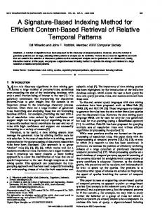
and polygons. Attributes consist of a geometry type identifier (SDO GTYPE), a Spatial reference system identifier (sdo srid), an element descriptor array (sdo elem info), and an ordinate array (sdo ordinates) among others. Sdo ordinates contains the values for coordinate pairs or triples that define the vertices of the geometric elements. Sdo elem info defines how these ordinates should be assigned to the element or elements that constitute the geometry. Spatial offers two types of indexing techniques, Quad-Tree indexing and R-Tree indexing. The Oracle Spatial R-Tree is essentially an Optimised R∗ -Tree structure. The algorithms for create, insert, delete and query are based almost entirely on the R∗ -Tree algorithm while the create and query algorithms also include packing optimisation using the TGS, VAMSplit, STR and other unpublished algorithms. Oracle 9i further introduced support for the function-based spatial indexes used in this implementation. Oracle 9i Release 2, added functionality to allow parallel creation of R-Trees and boasts performance enhancements of up to 50% in index creation and up to 40% with spatial queries using secondary filters.

Figure 10: Oracle Spatial: Query Model Spatial uses a two-tier Query Model to resolve spatial queries, as shown in Figure 10 (Murray 2002). The first operation, called Primary Filter, is implemented using the SDO FILTER function. It is a low cost filter that compares geometry approximations to return a superset of the exact result set. The second operation, called Secondary Filter, is implemented using the computationally expensive sdo relate function and is applied to the result set of the primary filter to yield an accurate answer to a spatial query. The R-tree index is responsible mainly for the primary filter while the Secondary Filter combines RTree based pruning (SDO FILTER) and geometrygeometry comparisons. Thus, the performance of both filters is studied as part of the implementation. A method of the SDO GEOMETRY type provided by Spatial and used in the implementation to exploit the computational advantage of the POINT approach, is the get gtype method which takes the geometry as input and returns the geometry type as per the sdo gtype parameter. Sample code for Query 1 for both approaches is provided bellow: @read_start_parameters select count(position) from max10 s where (sdo_filter(get_max_geo( s.Vts, s.Vte, s.Tts, s.Tte), get_max_ge(sysdate, sysdate, ‘31-DEC-9999’, ‘31-DEC-9999’), ‘querytype = WINDOW’ )=‘TRUE’ ); @read_end_parameters This query finds all geometries that intersect with the point (sysdate, ‘31-DEC-9999’). It uses the function get max geo which takes coordinates (V t` , V ta , T ta , T t` ) as input returns the corresponding geometry of sdo geom type.

@read_start_parameters select count(position) from point10 s where ((get_same_geo(s.Vts, s.Vte, s.Tts, s.Tte).get_gtype()=1 AND sdo_filter(get_same_geo( s.Vts, s.Vte, s.Tts, s.Tte), get_same_geo( 0, sysdate, 0 , sysdate), ’querytype = WINDOW’ )=’TRUE’) OR (get_same_geo(s.Vts, s.Vte, s.Tts, s.Tte).get_gtype()=2 AND sdo_filter(get_same_geo( s.Vts, s.Vte, s.Tts, s.Tte), get_same_geo( sysdate, sysdate, 0, sysdate), ’querytype = WINDOW’ )=’TRUE’) ); @read_end_parameters This query finds all point geometries (type 1) that are within the region (0, sysdate, 0, sysdate) and all line geometries (type 2) that intersect with the line defined by (sysdate, sysdate, 0, sysdate). It uses the function get same geo, which takes coordinates (attributes of the table point10 (Vts, Vte, Tts, Tte)) as input and returns the corresponding geometry type while taking care that different geometry types (i.e. points, lines and rectangles) are explicitly defined. As mentioned earlier, rectangle geometries (type 3) are not of interest for Query 1. Full query statements and scripts used for the population of data and index creations can be found in (Stantic & Khanna 2003). A series of problems were encountered during the implementation and analysis, such as undocumented memory bugs in Spatial and unexplained structural details critical for analysis. Considerable support was sought and provided from Oracle staff. Some of these solutions were documented for the benefit of future research, and can be found at (Stantic & Khanna 2003). 5.3

Analysis

The Query Performance results for Query 1, (see Figures 11 and 12), support the earlier hypothesis that the straightforward maximum-timestamp (MAX ) approach is inefficient in the handling of now-relative data. This inefficiency increases as the amount of now-relative data grows. Conversely, the POINT approach proved to be extremely efficient for the handling of now-relative data, with little or no effect from growing now-relative data, to the extent of outperforming the Spatial MAX approach by more than a factor of 20 in terms of the number of disk accesses. The better performance of the POINT approach is achieved by reducing the dimensions of the spatial geometries. Typically, rectangles representing nowrelative data are represented as lines or points, which take up less room in the leaf nodes than the original rectangles, leading to higher fan-out. The smaller dimensions of these geometries means there is less overlap between the maximum bounding regions, which form the boundaries of each node. In addition, because the representation of now-relative data in general does not extend beyond the current time, the amount of dead space (nodes that are searched but do not contribute to the answer) is reduced. Another explanation for the better performance of the POINT approach is its reduction of the search space, due to logically dividing the total space to the areas of interest and identifying only the geometry types of interest, which improves the performance significantly.

Approach Max Point Max Point Max Point

percentage 10% 10% 20% 20% 40% 40%

Disk Accesses 180353 142478 165980 92560 75038 35155

CPU 30291 47740 29538 65366 12134 31374

Table 7: Query 3: Disk Accesses and CPU usage

Figure 11: Query 1: Disk Accesses - Secondary Filter

worse for the POINT approach due to the complex logical query transformations. In addition to the select command, we tested the performance of the create, update and delete commands for both approaches using different quantities of now-relative data. The update performance, although not affected by the quantity of now-relative data, was greatly affected by the representation used. Similarly for the create command’s performance, the MAX approach consistently proved to be twice as computationally expensive in terms of CPU reads and significantly more expensive in terms of disk accesses. We could not identify any significant influence of parameters, such as size and tolerance of SGA, on the performance of the two methods tested. The space used for the POINT approach index structure is significantly smaller, as is the number of disk accesses and CPU usage during the initial index creation. 6

Conclusion and Future Work

This study makes the following contributions to the field: • We presented a method to efficiently index nowrelative bitemporal data by using the POINT approach, and • empirically demonstrated it to be an improvement, outperforming the Spatial MAX approach by a factor of over 20. • we found support for the previous hypothesis that a straightforward maximum-timestamp approach has poor performance; • the proposed method is based only on logical transformations of queries without the need for modification to the kernel, so an off-the-shelf spatial index can be used; Figure 12: Query 1: CPU Usage - Secondary Filter Approach Max Point Max Point Max Point

percentage 10% 10% 20% 20% 40% 40%

Disk Accesses 138147 127030 157983 67598 186681 30507

CPU 34111 45071 27681 42462 22925 38605

Table 6: Query 2: Disk Accesses and CPU usage The experimental results for Queries 2 and 3, shown in Tables 6 and 7, demonstrate that the POINT approach also has better performance in terms of disk accesses. Its relative performance, compared to the MAX approach, improves with larger amounts of now-relative data. As for Query 1, this can be explained by the reduction of both the maximum bounding regions, dead space, and a logical reduction of search space. However the CPU usage is

• we extended the spatiotemporal query notation for bitemporal databases, to better define range and timeslice queries; • we defined the domain of bitemporal tuples for different representations of now ; • we surveyed existing proposed spatial access methods to assess their effectiveness for indexing bitemporal data including now-relative data. • we identified the type and level of support offered by commercial databases for indexing spatial data. In future work, the advantages of the POINT approach for indexing now-relative bitemporal data could be employed to create a new more efficient access method. It would also be interesting to investigate the effectiveness of the POINT approach on other types of queries, such as interval queries.

References Bliujute, R., Jensen, C. S., Saltenis, S. & Slivinskas, G. (1998), R-Tree Based Indexing of Now-Relative Bitemporal Data, in ‘Proceedings of 24rd International Conference on Very Large Databases (VLDB’98)’, New York, USA, pp. 345–356. Bliujute, R., Jensen, C. S., Saltenis, S. & Slivinskas, G. (2000), Light-weight Indexing of General Bitemporal Data, in ‘Statistical and Scientific Database Management’, pp. 125–138. Clifford, J., Dyreson, C., Isakowitz, T., Jensen, C. S. & Snodgrass, R. T. (1997), ‘On the semantics of “Now” in databases’, ACM Transactions on Database Systems (TODS) 22(2), 171–214. Date, C., Darwen, H. & Lorentzos, N. (2002), Temporal Data and the Relational Model, Morgan Kaufmann. Dyreson, C. E., Snodgrass, R. T. & Freiman, M. (1995), Efficiently Supporting Temporal Granularities in a DBMS, Technical Report TR 95/07. URL: citeseer.nj.nec.com/dyreson95efficiently.html Gaede, V. & Gunther, O. (1998), ‘Multidimensional Access Methods’, ACM Computing Surveys (CSUR) 30(2), 170–231. Green, C. D. (2002), ‘Oracle9i Database Performance Tuning Guide and Reference, Release 2 (9.2) Part No. A96533-02’. URL: http://downloadwest.oracle.com/docs/cd/ B10501 01/server.920/a96533/title.htm Hellerstein, J., Koutsupias, E. & Papadimitriou, C. (1997), ‘On the Analysis of Indexing Schemes’, 16th ACM SIGACT-SIGMOD-SIGART Symposium on Principles of Database Systems . Jensen, C. S. (2000), ‘Introduction to temporal databases, research’, http://www.cs.auc.dk/ csj/Thesis/pdf/ chapter1.pdf . Jensen, C. S. & Snodgrass, R. (1999), ‘Temporal Data Management’, IEEE Transactions on Knowledge and Data Engineering 11(1), 36–44. Kleinrock, L. (1975), Queueing Systems: Theory, Vol. 1, 1 edn, John Wiley and Sons. Kumar, A., Tsotras, V. J. & Faloutsos, C. (1997), ‘Designing access methods for bitemporal databases’, University of Maryland at College Park; Report No. UMIACS-TR-97-24 . Murray, C. (2002), ‘Oracle Spatial User’s Guide and Reference, Release 9.2 Part No. A96630-01’. URL: http://downloadwest.oracle.com/docs/cd/ B10501 01/appdev.920/a96630/title.htm Salzberg, B. & Tsotras, V. J. (1999), ‘Comparison of Access Methods for Time Evolving Data’, ACM Computiong Surveys 31(1). Snodgras, R. & et al. (1987), ‘The Temporal Query Language TQEL’, ACM TODS 12(2), 247–298. Snodgrass, R. & Ahn, I. (1986), ‘Temporal databases’, IEEE Computer 19(9), 35–42. Snodgrass, R. T. (2000), Developing Time-Oriented Database Applications in SQL, Morgan Kaufmann.

Stantic, B. & Khanna, S. (2003), ‘The POINT representation of now in Temporal Databases’. URL: http://miami.int.gu.edu.au/POINT/ Stantic, B., Thornton, J. & Sattar, A. (2003), A Novel Approach to Model NOW in Temporal Databases, in ‘Proceedings of the 10th International Symposium on Temporal Representation and Reasoning (TIME-ICTL 2003)’, Cairns, Australia, pp. 174–181. Torp, K., Jensen, C. S. & Snodgrass, R. T. (1997), ‘Stratum Approaches to Temporal DBMS Implementation’, A TIMECENTER Technical Report . Tsotras, V. J., Jensen, C. S. & Snodgrass, R. T. (1998), ‘An Extensible Notation for Spatiotemporal Index Queries’, ACM SIGMOD Record 27(1), 47–53.