Efficient Informative Sensing using Multiple Robots - arXiv

Journal of Artificial Intelligence Research 34 (2009) 707-755

Submitted 08/08; published 04/09

Efficient Informative Sensing using Multiple Robots Amarjeet Singh Andreas Krause Carlos Guestrin William J. Kaiser

AMARJEET @ EE . UCLA . EDU KRAUSEA @ CALTECH . EDU GUESTRIN @ CS . CMU . EDU KAISER @ EE . UCLA . EDU

Abstract The need for efficient monitoring of spatio-temporal dynamics in large environmental applications, such as the water quality monitoring in rivers and lakes, motivates the use of robotic sensors in order to achieve sufficient spatial coverage. Typically, these robots have bounded resources, such as limited battery or limited amounts of time to obtain measurements. Thus, careful coordination of their paths is required in order to maximize the amount of information collected, while respecting the resource constraints. In this paper, we present an efficient approach for near-optimally solving the NP-hard optimization problem of planning such informative paths. In particular, we first develop eSIP (efficient Single-robot Informative Path planning), an approximation algorithm for optimizing the path of a single robot. Hereby, we use a Gaussian Process to model the underlying phenomenon, and use the mutual information between the visited locations and remainder of the space to quantify the amount of information collected. We prove that the mutual information collected using paths obtained by using eSIP is close to the information obtained by an optimal solution. We then provide a general technique, sequential allocation, which can be used to extend any single robot planning algorithm, such as eSIP, for the multi-robot problem. This procedure approximately generalizes any guarantees for the single-robot problem to the multi-robot case. We extensively evaluate the effectiveness of our approach on several experiments performed in-field for two important environmental sensing applications, lake and river monitoring, and simulation experiments performed using several real world sensor network data sets.

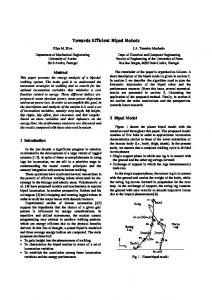
1. Introduction Global climate change and corresponding impetus on sustainable practices for environment-related activities has brought forth the challenging task of observing natural phenomena exhibiting dynamics in both space and time. Observing and characterizing these dynamics with high fidelity will be critical for answering several questions related to policy issues for monitoring and control and understanding biological effects on activity of microbes and other organisms living in (or dependent on) these environments. Monitoring algal bloom growth in lakes and salt concentration in rivers, as illustrated in Fig. 1, are specific examples of related phenomena of interest to biologists and other environment scientists (MacIntyre, 1993; Ishikawa & Tanaka, 1993; MacIntyre, Romero, & Kling, 2002). Monitoring environmental phenomena, such as algal bloom growth in a lake, requires measuring physical processes, such as nutrient concentration, wind effects and solar radiation, among others, across the entire spatial domain. One option to acquire data about such processes would be to statically deploy a set of sensing buoys (Reynolds-Fleming, Fleming, & Luettich, 2004). Due to the large spatial extent of the observed phenomena, this approach would require a large number of sensors in order to obtain high fidelity data. The spatio-temporal dynamics in these environments

c

2009 AI Access Foundation. All rights reserved.

S INGH , K RAUSE , G UESTRIN & K AISER

(a) Confluence of San Joaquin and Merced River

(b) Lake Fulmor, San Jacinto mountain reserve

Figure 1: Deployment sites used for performing path planning in-field. motivate the use of actuated sensors – robots carrying sensors together with an efficient approach for planning the paths of these actuated sensors. These actuated sensors have been used in the past (Dhariwal et al., 2006) for measuring the phenomena at various locations and hence providing the biologists with critical information about the state of the lake. Typically however, such robots have strict resource constraints, such as storage battery energy, that limits the distance they can travel or the number of measurements they can acquire before the observed phenomena varies significantly. These constraints necessitate careful motion planning for the robots – coordinating their paths in order to maximize the amount of collected information, while satisfying the given resource constraints. In this paper, we tackle this important problem of seeking informative paths for a collection of robots, subject to constraints on the cost incurred by each robot, e.g. due to limited battery capacity. In order to optimize the paths of these robots, we first need to quantify the informativeness of any particular chosen path. In this work, we adopt an approach from spatial statistics and employ probabilistic models of the spatial phenomena. Using these models, informativeness can be viewed in terms of the uncertainty about our prediction of the phenomena at unobserved locations, given the observations made by the mobile robots at a subset of locations (the selected path). In particular, we use a rich class of probabilistic models called Gaussian Processes (GPs) (Rasmussen & Williams, 2006) that has been shown to accurately model many spatial phenomena (Cressie, 1991), and apply the mutual information (MI) criterion (Caselton & Zidek, 1984) to quantify the reduction in uncertainty achieved through selected robot paths. Unfortunately, the problem of finding an optimal collection of paths, maximizing the mutual information criterion, is an NP-hard search problem, which is typically intractable even for small spatial phenomena. In this paper, we will develop an approximation algorithm which efficiently finds a provably near-optimal solution to this optimization problem. The key insight which will allow us to obtain such an algorithm is that the mutual information (and several other notions of informativeness (as discussed in Krause and Guestrin, 2007) satisfies submodularity, an intuitive diminishing returns property - making a new observation helps more if we have made only a few observations so far, and less if we have already made many observations (Krause et al., 2008). The problem of optimizing the path of a single robot to maximize a submodular function over the visited locations was studied by Chekuri and Pal (2005), who developed an algorithm, recursivegreedy, with strong theoretical approximation guarantees. Unfortunately, the running time of their 708

E FFICIENT I NFORMATIVE S ENSING USING M ULTIPLE ROBOTS

approach is quasi-polynomial: it scales as M log M , for M possible sensing locations. This property makes the algorithm impractical for most environmental sensing applications, with typical numbers (M ) of observation locations reaching to several hundreds and more. In this paper, we present two techniques – spatial decomposition and branch and bound search – for overcoming these limitations of the recursive-greedy approach of Chekuri et al., making it practical for real world sensing problems. We call this efficient approach for single robot path planning eSIP (efficient Single-robot Informative Path planning). We then provide a general approach, sequential-allocation, which can be used to extend any single robot algorithm, such as eSIP, to the multi-robot setting. We furthermore prove that this generalization only leads to minimal reduction (independent of the number of mobile robots) of the approximation guarantee provided by the single robot algorithm. We combine eSIP with sequentialallocation to develop the first efficient path planning algorithm (eMIP) that coordinates multiple robots, each having a resource constraint, in order to obtain highly informative paths, i.e. paths that maximize any given submodular function, such as mutual information. By exploiting submodularity, we prove strong theoretical approximation guarantees for our algorithm. We extensively evaluate the effectiveness of our approach on several experiments performed in-field for two important environmental sensing applications, lake and river monitoring. The river campaign was executed at the confluence of two rivers, Merced river and San Joaquin river, in California from August 7-11, 2007. Fig. 1a displays an aerial view of the San Joaquin deployment site. The lake campaign was executed at a lake located at the University of California, Merced campus from August 10-11, 2007. Fig. 1b displays an aerial view of lake Fulmor. In both campaigns, the Networked Info Mechanical System (NIMS) (Jordan et al., 2007), a cable based robotic system, was used to perform path planning while observing a two dimensional vertical plane (cross-section). In addition to analyzing data from these deployments, we provide extensive experimental analysis of our algorithm on several real world sensor network data sets, including the data collected using a robotic boat at lake Fulmor (Dhariwal et al., 2006). This manuscript is organized as follows. We formally introduce the Multi-robot Informative Path Planning (MIPP) problem in Section 2. In Section 3, we discuss the sequential-allocation approach for extending any single robot path planning algorithm to the multi-robot setting while preserving approximation guarantees. We then review the recursive-greedy algorithm proposed by Chekuri et al. (Section 5), an example of such a single-robot algorithm. Subsequently, we present our spatial decomposition (Section 6) and branch and bound techniques (Section 7) which drastically improve the running time of recursive-greedy and make it practical for real world sensing applications. In Section 8, we evaluate our approach through in-field experiments as well as in simulations on real world sensing datasets. In Section 9, we review related work, and we present our conclusions in Section 10. The proofs for all our results are presented in the Appendix.

2. The Multi-robot Informative Path Planning Problem We now formally define the Multi-robot Informative Path Planning (MIPP) problem. We assume that the spatial domain of the phenomenon is discretized into finitely many sensing locations V. For each subset A ⊆ V, let I(A) denote the sensing quality, i.e. the informativeness, of observing the phenomenon at locations A. Details on appropriate choices for the sensing quality I are given below. We also associate with each location v ∈ V, a sensing cost C(v) > 0, quantifying the expenses of obtaining a measurement at location v. When traveling between two locations, u and v, a robot in-

709


curs a traveling cost C(u, v) > 0. A robot traverses a path in this space: an s–t-path P is a sequence of l locations starting at node s, and finishing at t. The cost C(P) of path P = (s = vP 1 , v 2 , . . . , vl = l−1 t) is the sum of sensing costs and traveling costs along the path, i.e. C(P) = i=2 C(vi ) + Pl C(v , v ). In the case l = 2, cost of the path P will only involve traveling cost between the i−1 i i=2 starting and finishing locations C(s, t). We will use the notation P to both refer to the sequence of nodes in the path, and to the subset of sensing locations P ⊆ V (ignoring their sequence). For a collection of k paths P = {P1 , . . . , Pk }, one for each robot, I(P) = I(P1 ∪ · · · ∪ Pk ) denotes the sensing quality of the paths, which quantifies the amount of information collected by the k paths. The goal of the MIPP problem is to find a collection P of k paths, with specified starting and finishing location si and ti (not necessarily different), such that each path has bounded cost C(Pi ) ≤ B for some specified budget B, and that the paths are the most informative, i.e. I(P) is as large as possible. Formally, the problem can be defined as: max I(∪ki=1 Pi ); subject to C(Pi ) ≤ B, ∀ i ∈ {1, . . . , k}.

Pi ⊆V

(1)

In our lake monitoring example with the goal of performing surface monitoring using boats, we first discretized the two-dimensional surface of the lake into finitely many sensing locations (as depicted in Fig. 1b). For the single robot scenario, we then seek to find the most informative path P1 (in terms of predicting the algal bloom content) starting from location s and finishing in location t. The experiment cost C(vi ) corresponds to the energy required for making chlorophyll and related measurements (indicators of amount of algal bloom). The traveling cost C(vi−1 , vi ) corresponds to the energy consumption when traveling from location vi−1 to vi . The budget B quantifies the total energy stored in the boat’s battery. 2.1 Quantifying Informativeness: How can we quantify the sensing quality I? To model spatial phenomena, a common approach in spatial statistics is to use a rich class of probabilistic models called Gaussian Processes (GPs, c.f., Rasmussen and Williams, 2006). Such models associate a random variable Xv with each location v ∈ V. The joint distribution P (XV ) can then be used to quantify uncertainty in the prediction P (XV\A | XA = xA ) of phenomena at unobserved locations XV\A , after making observations XA = xA at a small subset A of locations. To quantify this uncertainty we use, for example, the mutual information (MI) criterion (as discussed by Caselton and Zidek, 1984). For a set of locations, P, the MI criterion is defined as: MI(A) ≡ H(XV\A ) − H(XV\A | XA )

(2)

where H(XV\A ) is the entropy of the unobserved locations V \ A, and H(XV\A | XA ) is the conditional entropy of locations V \ A after sensing at locations A. Hence mutual information measures the reduction in uncertainty at the unobserved locations. Therefore, in our lake monitoring example, we would like to select the locations that most reduce the uncertainty in the algal bloom content prediction for the lake environment. Conveniently, in a GP, the mutual information criterion can be computed efficiently and analytically (Caselton & Zidek, 1984). The effectiveness of mutual information to select informative sensing locations was studied by Krause et al. (2008). Several alternative information criteria such as entropy (Ko et al., 1995), information disk model (Bai et al., 2006) and alphabetical optimality criterion such as A-, D- and E-optimal have also been used to associate sensing quality with observation locations in related problem domain. 710


2.2 Submodularity: Even if we do not consider the constraints on the length of the paths of the robots, the problem of selecting locations that maximize mutual information is NP-hard (Krause et al., 2008). Hence, in general, we most likely cannot expect to be able to efficiently find the optimal set of locations. Instead, our goal will be to efficiently find near-optimal solutions, for which the sensing quality (e.g. mutual information), is provably close to the optimal sensing quality. The key observation, which will allow us to obtain such strong approximation guarantees, is that mutual information satisfies the following diminishing returns property (Krause et al., 2008): The more locations we have already sensed, the less information we will gain by sensing a new location. This intuition is formalized by the concept of submodularity: A function f is submodular (Nemhauser et al., 1978) if: ∀A ⊆ B ⊆ V and s ∈ V \ B; f (A ∪ s) − f (A) ≥ f (B ∪ s) − f (B).

(3)

Another intuitive property is that sensing quality is monotonic1 , which means that I(A) ≤ I(B) for all A ⊆ B ⊆ V. Hence, as we select more and more sensing locations, we will collect more and more information. Lastly, mutual information is normalized, i.e. I(∅) = 0. We thus define our MIPP problem as the problem of optimizing paths of length at most B for k robots, such that the selected sensing locations maximize a normalized, monotonic submodular function I(·). This definition of the MIPP problem allows our approach to be applied to any monotonic submodular objective function, not just mutual information. This generalization is very useful, as several other notions of informativeness can be shown to satisfy submodularity (Krause & Guestrin, 2007). 2.3 Online vs Offline Path Planning: Many robotic path planning applications, such as search and rescue, involve uncertain environments with complex dynamics that can only be partially observed. Informative path planning – selecting the best locations to observe subject to given sensing constraints, in such uncertain environments necessitates a trade off between exploration (gathering information about the environment) and exploitation (using the current belief about the state of the environment most effectively). We distinguish two different classes of algorithms: nonadaptive (offline) algorithms, that plan and commit to the paths before any observations are made, and adaptive (online) algorithms, that update and replan as new information is collected. Both the online and offline settings are NP-hard optimization problems. In this paper, we only discuss the approximation algorithms for the offline setting that exploit the known belief about the environment for efficient path planning. We plan to work towards extending our approach for an exploration-exploitation trade-off to incorporate online model adaptation in the future.

3. Approximation Algorithm for MIPP The problem of optimizing the path of a single robot (i.e. k = 1) to maximize a submodular function of the visited locations, constrained by an upper bound (B) on the path cost, was first studied by Chekuri and Pal (2005). We will review their recursive-greedy algorithm in detail in Section 5. 1. This monotonicity holds only approximately for mutual information (Krause et al., 2008), which however is sufficient for all purposes of this paper.

711


1

Algorithm:sequential-allocation

Input: B, k, starting / finishing locations s1 , . . . , sk , t1 , . . . , tk , V Output: A set of informative paths P1 , . . . , Pn 2 begin 3 A0 ← ∅; 4 for 1 ≤ i ≤ k do // Performing path planning for the ith robot 5 Pi ← SP P (si , ti , B, Ai−1 , V); // Committing to the previously selected locations 6 Ai ← Ai−1 ∪ Pi ; 7 return P1 , . . . , Pk ; 8 end Algorithm 1: Sequential allocation algorithm for multi robot path planning using any single robot path planning algorithm SPP. Output set of paths P1 , . . . , Pk provides an approximation guarantee of 1 + η where η is the approximation guarantee of single robot path planning algorithm SP P .

In our lake monitoring problem, we seek to plan multiple paths, one for each robot. One possibility is to apply the single-path algorithm to the product graph, i.e. plan a path over tuples of locations simultaneously representing the locations of all robots. However, such straightforward application of the single-robot planning algorithm would lead to an increase in running time which is exponential in the number of robots, and therefore intractable in practice. We are not aware of any sub-exponential approximation algorithm for this challenging multiple-robot path planning problem. In this paper, we present a simple algorithm for the multi-robot scenario that can exploit any approximation algorithm for the single robot case, such as the recursive-greedy algorithm, as discussed by Chekuri and Pal (2005), and (almost) preserve the approximation guarantee, while avoiding the exponential increase in running time. Our algorithm, sequential-allocation, successively applies the single robot path planning algorithm k times to get the paths for k robots. Hereby, when planning the jth path, the approach takes into account the locations already selected by the previous j − 1 paths. Committing to the (approximately) best possible path at each stage before moving on to the next stage makes our approach “greedy” in terms of paths. The pseudocode of the algorithm is presented in Algorithm 1 and Fig. 2 illustrates the approach for three robots. The algorithm takes as input the budget constraint B, number of available robots k, starting and finishing location for each available robot s1 , . . . , sk , t1 , . . . , tk and the complete set of discrete observation locations V to select from. Let us assume that we have a single robot path planning algorithm, SP P , that takes as input a starting location si , a finishing location ti , budget constraint B, a set of locations already selected for observation and a set of possible observation locations that can be visited. In Fig. 2, all the three robots have same starting and finishing location. While planning the path for the first robot (i = 1), the input set of already selected observation locations is empty. At each subsequent stage, we commit to the locations selected in all the previous stages and pass the already observed locations as input to our next call to SP P . Let Ai−1 be the locations already visited by paths P1 , . . . , Pi−1 , and A0 = ∅. Then the residual information, IAi−1 for a path P over unvisited locations is defined as IAi−1 (P) = I(Ai−1 ∪P)−I(Ai−1 ). It can be verified that if I is a normalized, monotonic and submodular function, then so is the residual information 712


Figure 2: Illustration of sequential allocation algorithm for three robots, each with the same starting and finishing location.

IAi−1 . Thus, at stage i we use SP P to find the most informative path with respect to the modified residual sensing quality function. In Fig. 2, when planning P2 , locations selected for P1 are considered and the sensing quality function used is IP1 . Similarly, while evaluating the path P3 , locations selected for P1 and P2 are taken into account and the sensing quality function used is IP1 ∪P2 . Perhaps surprisingly, this straight-forward “greedy” sequential allocation approach is guaranteed to perform almost as well as the black box algorithm used for path planning. More formally, assume we have an η -approximate algorithm for the single robot problem, i.e. an algorithm which, starting with budget B and a monotonic submodular function f , is guaranteed to find a path recovering at least a fraction of 1/η of the optimal information achievable with the same budget. In this case, the following theorem proves that the sequential allocation procedure has approximation guarantee close to η as well: Theorem 1. Let η be the approximation guarantee for the single path instance of the informative path planning problem. Then our sequential-allocation algorithm achieves an approximation guarantee of (1 + η) for the MIPP problem. In the special case, where all robots have the same starting (si = sj , ∀i, j) and finishing locations (ti = tj , ∀i, j), the approximation guarantee improves to 1/(1 − exp (−1/η)) ≤ 1 + η. The work by Blum et al. (2003) proved Theorem 1 for the special case of additive (modular) sensing quality functions. In this paper, we extend their result to general submodular functions. As an example of an η-approximate algorithm for the single robot problem, in the next section, we review the recursive-greedy algorithm as proposed by Chekuri and Pal (2005). This algorithm has an approximation guarantee η of O(log2 |P ∗ |), where |P ∗ | is the number of locations visited by an optimal solution P ∗ . Hence, for this algorithm, the performance guarantee obtained for the MIPP problem through sequential allocation is O(log2 |P ∗ |) as well2 . 2. In order to apply sequential allocation to the recursive-greedy algorithm, we can, when planning the ith path, simply pass the set of nodes visited by the previous i − 1 paths as the input parameter R, as is illustrated in Algorithm 2.

713


(a)

(b)

(c)

(d)

Figure 3: Illustration of performance of simple greedy approaches compared to an optimal approach.

4. A Note on Greedy Path Planning The work by Krause et al. (2008) considered the sensor placement problem, where a subset A ⊆ V of k locations is selected in order to maximize the mutual information, without considering path costs. By exploiting the submodularity property of MI, they proved that if the discretization V is fine enough and the GP satisfies mild regularity conditions, greedily selecting locations based on this criterion is near-optimal. More specifically, the greedy algorithm (which we call GreedySubset in the following), after selecting the first i locations Ai , picks the location with maximum residual information i.e. vi+1 = argmaxv IAi ({v}) and sets Ai+1 = Ai ∪ {vi+1 }. GreedySubset hence iteratively adds locations which increase mutual information the most. Using a result proposed by Nemhauser et al. (1978) on the performance of the greedy algorithm for submodular functions, the work by Krause et al. (2008) showed that GreedySubset selects sets which achieve mutual information of at least (1 − 1/e) OPT −ε, where OPT is the optimal mutual information among all sets of the same size, and ε is a small error incurred due to the discretization. The strong performance of the greedy algorithm in the unconstrained (no traveling costs between locations) case motivates the question of whether a simple greedy approach could perform well in the more complex path planning setting considered in this paper. While it is difficult to give a general impossibility statement for such a question, several natural extensions of the greedy algorithm can be shown to perform arbitrarily badly. For example, consider a setting where we define the cost C(A) of a set of nodes as the cost of the cheapest path connecting the nodes A. Assuming locations Ai have already been picked, a natural extension of the greedy algorithm will be to add a location v which most improves the benefit-cost ratio IA (v) v ∗ = argmax i , v∈V\A CAi (v) 714


where CAi (v) = C(Ai ∪ {v}) − C(Ai ) is the increase in cost after adding v to the already selected locations Ai . Fig. 3 shows a small example illustrating that this intuitive greedy procedure can perform arbitrarily poorly compared to an optimal approach. The example is illustrated in Fig. 3a, with s as both the starting and the finishing location and 2B as the total available budget. The reward associated with each observation location is displayed in parenthesis with the corresponding locations. For the ease of illustration, we assume that the reward associated with each observation location is some modular function (instead of a submodular function). Traveling cost is associated with the corresponding edges in the example. Starting at location s, possible options for the first observation location are to select either of o1 , g1 or t. Observation location o1 will lead to a cluster of n (= B/) locations each separated by a traveling cost and with an associated reward of 1 (except o1 that has an associated reward of ). o1 is separated from g1 by a traveling cost of B/2 while the rest of the locations in the cluster are assumed to be unreachable from any other location outside the cluster. Observation location g1 will lead to a series of m (= B/) locations, each separated from the previous one by traveling cost and with an associated reward of 2. As illustrated in Fig. 3b, an optimal approach would select o1 as the first location, paying a traveling cost of B/2 and earning a very small reward . Once the robot observes o1 , it can then observe the rest of (B/ − 1) locations in the cluster, each providing a reward of 1 and return back to s while spending a total of 2B as the traveling cost. Thus, the total reward collected by an optimal approach, for this example, will be 1(B/ − 1) + . As illustrated in Fig. 3c, a “greedy” approach based on the reward-cost ratio will select g1 as the first observation location (with the highest reward to cost ratio of 2). Since o1 is at a distance B/2 away from g1 and only provides a reward of , this approach will continue along the series, observing all the locations till gm and returning back to s. Total reward collected by such an approach will be 2B. On the other hand, a simple “greedy” approach based on reward (as illustrated in Fig. 3d) will simply select t as the first observation location and return back to s, collecting a total reward of 1. Since the ratio B/ can be arbitrarily large as → 0, the reward collected by simple intuitive greedy approaches (2B or 1) can be arbitrarily poor when compared to the reward collected by an optimal approach (1(B/ − 1) + ). Although, the reward function considered in the example was assumed to be a modular function, the submodular optimal reward can also be arbitrarily large, compared to submodular reward collected by simple greedy approaches (the difference between the submodular and modular reward will depend on the correlation of the selected observation locations). This insight necessitates the development of more complex algorithms for path planning as considered in this paper.

5. The Recursive-greedy Algorithm We will now review the recursive-greedy algorithm as proposed by Chekuri and Pal, since it forms the basis for our efficient single robot path planning approach. The basic strategy of the algorithm is a divide-and-conquer approach. Any path from the starting location (s) to finishing location (t) has a middle location (vm ) such that there are same number of locations (or different by at most 1) on either side of vm in the s − t path. Thus, the problem of finding a s − t path can be divided into two smaller subproblems of finding smaller subpaths (s − vm and vm − t) and then concatenating these small subpaths. While having the same number of locations, the subpaths on either side of the middle node can have different costs, i.e. the budget for the total path has to be split into two smaller

715


1

Algorithm:recursive-greedy (RG)

Input: s,t,B,R,iter Output: An informative path P 2 begin 3 if c(s, t) > B then 4 return Infeasible; 5 P ← s, t; 6 Base case: iter=0 return P; 7 m ← fR (P); // Trying each location as middle node 8 foreach vm ∈ V do // Trying all possible budget splits 9 for 1 ≤ B1 ≤ B do // Planning subpath on one side of the middle node 10 P1 ← RG(s, vm , B1 , R, iter − 1); // Planning subpath on other side of the middle node, committing to nodes selected in first subpath 11 P2 ← RG(vm , t, B − B1 , R ∪ P1 , iter − 1); 12 if fR (P1 ∪ P2 ) > m then 13 P ← P1 ∪ P2 ; 14 m ← fR (P); 15 return P; 16 end Algorithm 2: Recursive greedy algorithm for single robot instance of MIPP as proposed by Chekuri and Pal (2005). Output path P provides an approximation guarantee of IX (P) ≥ IX (P ∗ )/ d1 + log ke, where I represent the submodular reward function, P ∗ represent an optimal path and k represent the number of nodes in the optimal path.

budgets (not necessarily equal), one for each subpath. Searching for the best middle location and trying all possible budget splits on either side of the middle location, while optimizing the complete s − t path, would result in an exhaustive search for the optimal solution and therefore will be prohibitively expensive. Instead of performing this exhaustive search, the recursive-greedy algorithm follows a simple greedy strategy, wherein for each of the possible budget splits and each possible middle nodes considered, one can first plan the optimal subpath on one side of the middle location, then commit to the planned subpath and optimize for the subpath on the other side. Such a path, consisting of independently optimized subpath s−vm and a subpath vm −t optimized subject to observation locations already selected in s − vm , may result in a suboptimal s − t path. Nonetheless, Chekuri and Pal proved that such a path has an approximation guarantee of O(log2 |P ∗ |), where |P ∗ | is the number of locations visited by an optimal solution P ∗ . In order to implement such a greedy approach, the recursive calls planning the second subpath will – similarly as done in sequential allocation – optimize a residual reward function which measures the incremental gain taking into account the information already obtained by the locations selected in the first subpath. More formally, let the set P1 refer to the locations selected in the first subpath, and consider the residual submodular function fP1 over a set of locations A as 716


fP1 (A) = f (A ∪ P1 ) − f (P1 ). If P2 is the set of locations in the second subpath, then it holds that f (P1 ) + fP1 (P2 ) = f (P1 ∪ P2 ). Hence, if the first recursive call (with submodular function f ) returns path P1 , and the second recursive call (with submodular function fP1 ) returns path P2 , then the sum of the scores of the subproblems exactly equals the score of the concatenated path. Let us now formalize the intuitive description of the recursive-greedy algorithm. The pseudocode of the algorithm is presented in Algorithm 2. The inputs to the algorithm are a starting location s, a finishing location t, an upper bound on the path cost B, a parameter R that defines the residual for the submodular function such that the function that needs to be maximized is defined as fR (P) = f (P ∪ R) − f (R), and a parameter i that represents the recursion depth. The maximum number of locations that can be selected at each stage is calculated using the recursion depth as 2i . In the base case (recursion depth i = 0), the algorithm simply returns the path P = (s, t) (if the cost c(s, t) ≤ B). In the recursive case, the algorithm searches for a s − t path with maximum reward by iterating over all possible locations (that can be reached with given budget constraint) as middle locations (Line 8), i.e. locations that could possibly split the required path into two subpaths with equal number of locations on either side. For each such middle location, the algorithm explores all possible splits of available budget (Line 9) across the two subpaths on either side of the middle location. Reducing the recursion depth by 1, for each subpath, ensures that the same number of locations are selected on either side of the middle location. However, before exploring the second subpath, the algorithm commits to the locations selected in the first subpath by passing them as input through the “residual” parameter (Line 11). The two subpaths found in such a way are then concatenated to provide a complete s − t path. The algorithm stores the best possible s − t path over the already searched problem space, replacing it with a better path whenever such a path is found. 5.1 Structure of the Search Problem It is instructive to consider the recursive structure generated by the recursive-greedy algorithm. Fig. 4 illustrates an example of such a structure when running recursive-greedy for our lake sensing application with the given starting (s) and finishing (t) location and an upper bound on the path cost (B). The search using recursive-greedy can be represented graphically as a sum-max tree. At the root is a max node representing the objective of finding a s − t path with maximum possible reward, while the cost of the path is bounded by budget B. For each such max node, the children in the search tree represent sum nodes corresponding to sum of rewards collected from the two subpaths on either side of the middle location. Therefore, at the end of the first iteration, the graphical representation will have a max node as root with several sum nodes as children, for each feasible middle location and each possible budget splits around that middle location. A partial tree at the end of first iteration is shown in Fig. 4a. For each sum node, formed at the end of the first iteration, the algorithm is then applied recursively on the left subpath. Thus the first step of second iteration seeks to find a s − vm path with maximum possible reward under the budget constraint corresponding to the respective budget split for the sum node. Then, their approach commits to the selected locations on the left side, and recurses on the right subpath (to search for a vm − t path), given these selected locations. As a result, each sum node will have two max nodes as children, each representing an objective to find a subpath of maximum reward on either side of the selected middle location. This algorithm is “greedy” in that it commits to the locations selected in the first subpath before optimizing the second subpath.

717


(a) recursive-greedy during first iteration

(b) recursive-greedy during second iteration

Figure 4: Illustration of recursive greedy algorithm, as proposed by Chekuri and Pal, for the lake sensing application. Sum-max tree presents the graphical representation of the problem space.

A partial tree at the end of second iteration is shown in Fig. 4b. Despite the greedy nature, the recursive-greedy approach provides the following approximation guarantee: Theorem 2. (Chekuri & Pal, 2005) Let P ∗ = (s = v0 , v1 , . . . , vk = t) be an optimal s-t-path solution. Let P be the path returned by RG(s, t, B, R, i). If i ≥ d1 + log ke, then IX (P) ≥ IX (P ∗ )/ d1 + log ke. 1 Hence, the recursive-greedy solution P obtains at least a fraction of d1+log of the optimal 2 ke information, where k ≤ n, i.e. the total number of locations traversed by the optimal path will be smaller than the total number of locations in the discretized spatial domain. Referring back to Theorem 1, for the MIPP problem using recursive-greedy as the single robot path planning approach, η = d1 + log ke.

5.2 Running Time By inspecting the recursive structure, the running time of the recursive-greedy algorithm can be seen to be quasi-polynomial. More specifically, the running time of the algorithm is O((M B)O(log2 M ) ), where B is the budget constraint and M = |V| is the total number of possible observation locations. So, even for a small problem with M = 64 locations, the exponent will be 6, resulting in a very large computation time, making the algorithm impractical for observing several real world physical processes. The large computational effort required by recursive-greedy can be attributed to two issues: 1) the large branching factor at each of the max nodes of the recursion tree (sum nodes for each possible middle node and each possible budget split across that middle node) and 2) (possibly) unnecessary recursion while exploring subtrees in problem space that can not provide us with an improved reward compared to current best solution. In the following sections, we propose two complementary approaches (can be used independently of the others) which are intended to ameliorate these concerns: a spatial decomposition technique, and a branch and bound approach. Spatial decomposition 718


Starting node s

Starting cell Cs

Ending node t

Ending cell Ct

Cs

Middle cell Cm Ct P1, budget = B’ P2, budget = Be–B’

Incoming path P1

a

b

(a) Spatial decomposition of the phenomenon

d

c

Smoothed path

Exiting path P2

Cell center

(b) Cell paths and travel within cells

(c) Cell paths and path smoothing

Figure 5: Illustration of spatial decomposition in recursive-eSIP using surface sensing in lake environment as an example. The sensing domain ((a), top) is decomposed into a grid of cells ((a), bottom). recursive-eSIP jointly optimizes over cell-paths ((b), top) and allocations of experiments in the cells ((b), bottom). Within the cells, locations are connected to cell center. recursive-eSIP concatenates paths between-cell and within cell paths ((c), top) and finally heuristics are applied in eMIP to smooth the path ((c), bottom). (discussed in Section 6) seeks to reduce the high branching factor (i.e. the number of sum nodes in the search tree) by clustering the sensing locations and then running the recursive-greedy over these clusters instead of actual sensing locations. Branch and bound (discussed in Section 7) seeks to avoid unnecessary recursion by maintaining a lower and an upper bound on the possible reward from a subtree in the search tree and pruning the tree accordingly. These two approaches, together with sequential-allocation (discussed in Section 3) provide an efficient algorithm for multi robot informative path planning.

6. Spatial Decomposition – Approximating MIPP as SD-MIPP In this section, we explain in detail the process of spatial decomposition and the corresponding improvements in running time achieved through this process. Our approach assumes that the traveling cost between arbitrary locations is given by their euclidean distance. An intuitive approach for improving the running time is to spatially decompose the sensing region into smaller sub-regions, each containing a cluster of sensing locations. We can thus think about planning informative paths as deciding which sub-regions to explore, and then deciding which locations to sense within these sub-regions. The idea of exploring the sub-regions motivates the decomposition of the sensing domain into smaller regions (cells). We can then run the recursivegreedy algorithm on these cells instead of the actual sensing locations. Since the size of each cellular region is small, traveling cost within each cell can be ignored3 . Once we ignore the traveling cost within the cells, sensing locations inside the selected cells can be chosen using the GreedySubset approach (as proposed by Krause et al., 2008), taking advantage of its strong approximation guar3. There may be robotic platforms where non-holonomic motion constraints will make small motions much more challenging and thus traveling cost for smaller distances within a cell may become non-negligible. For such systems, with large traveling cost for smaller motions, some system specific constraints may be possible to account for while performing cellular decomposition or the greedy algorithm may be constrained to not select locations that are “too” close).

719


antee in an unconstrained setting as discussed in Section 4. Fig. 5 presents an illustration of our approach and is explained as follows: 1. We decompose the sensing region, containing finitely many discrete sensing locations (c.f., e = {C1 , C2 , . . . , CN } (c.f., Fig. 5a, Fig. 5a, top), into a collection of non-overlapping cells V bottom). The distance between two cells is defined as the distance between the centroids of these cells. Each cell Ci contains a set of locations vi ∈ V, representing sensing locations, such that the coordinates of these locations, in a euclidean metric space, lie within the boundary of the containing cell. 2. We approximate the original MIPP problem with the spatially decomposed MIPP problem, or e In SD-MIPP, we jointly optimize over cell-paths in V e (c.f., Fig. 5b, SD-MIPP problem on V. top) using the recursive-greedy algorithm, and over the allocation of observations within the cells visited by the paths using the GreedySubset algorithm. Thus, when allocating measurements to a cell, we ignore the traveling cost within the cell (c.f., Fig. 5b, bottom). Since the cells are not very large, this simplification only leads to a small additional cost when the SD-MIPP solution is transformed back to the original MIPP problem. 3. We transfer the (approximate) SD-MIPP solution, consisting of a cell-path and an allocation of observations to cells (c.f., Fig. 5c, top), back to the original MIPP problem. We then smooth the path (c.f., Fig. 5c, bottom) using heuristics, e.g. the tour-opt heuristics as discussed by Lin (1965). Dual optimization of cell paths and budget allocation for observations within each visited cell motivated splitting the available budget Be into a budget Bt for traveling between the cells and a budget Be for making experiments at sensing locations within the visited cells. Such a split can be easily incorporated in recursive-greedy algorithm as well but was not required as the paths in recursivegreedy were optimized over observation locations and not cells containing these locations. Formally, the SD-MIPP problem is the following: We want to find a path PC∗ = (Cs = Ci1 , . . . , Cil = Ct ), for each robot i with starting cell Cs containing the starting node s and finishing cell Ct containing the finishing node t, with a travel cost of at most Bt . This travel budget is measured in terms of distances between centers of visited cells, and the cost of traveling within the cells is defined as 0. In addition, for each visited cell Cij in PC∗ , we want to select a set of sensing locations Aij , such that the total experimental cost (for making observations within the visited cells) is upper bounded by Be , i.e. C(Ai1 ∪ · · · ∪ Ail ) ≤ Be , and that the information I(Ai1 ∪ · · · ∪ Ail ) is as large as possible. The optimal SD-MIPP solution uses the optimal split of the budget Be into Bt and Be . To simplify the presentation, we rescale the costs such that the cells form a uniform grid of quadratic cells with width L, and assume that the sensing cost Cexp is constant over all locations. These assumptions can easily be relaxed, but they allow us to relate the path costs to the number of cells traversed, to simplify the discussion. The following lemma states that there exists an SD-MIPP version (PC∗ ) of the MIPP-optimal path (P ∗ ), with (almost) the same cost, and the same information. Lemma 3. Let P ∗ = (s = v0 , v1 , . . . , vl = t) be an optimal s-t-path solution to MIPP, constrained by budget B. Then there exists a corresponding SD-MIPP path PC∗ = (Cs = Ci1 , . . . , Cil = Ct ), √ traversing through locations Ai1 ∪ · · · ∪ Ail , with budget Be of at most 2 2B + 4L collecting the same information.

720


Algorithm: eMIP e k, starting / finishing locations s1 , . . . , sk , t1 , . . . , tk Input: B, Output: A collection of informative paths P1 , . . . , Pk 2 begin 3 Perform spatial decomposition into cells; 4 Find starting and ending cells Csi and Cti ; 5 R ← ∅; // Path planning for each robot 6 for i = 1 to k do // Trying different combination of traveling and experimental budget e do for iter = 0 to blog2 Bc 7 iter e 8 Be ← B − 2 ; 0 9 Piter ←recursive-eSIP (Csi , Cti ,Be ,R,iter); 0 10 Smooth Piter using tour-opt heuristics; 0 ); 11 Pi ← argmaxiter I(Piter 12 R ← R ∪ Pi ; 13 return P1 , . . . , Pk ; 14 end Algorithm 3: eMIP algorithm for informative multi robot path planning. Procedure from Line 7 to Line 11 1

effectively implements eSIP algorithm. eSIP is then repeated (Line 6) using sequential allocation described in Section 3 (Line 6) to get paths for each robot i.

We now present an algorithm for finding an approximately optimal solution to SD-MIPP, and then we show that this solution √ gives us an approximate solution to the original MIPP problem, with just slightly increased cost of 2 2B + 4L, for ensuring that the optimal solution for MIPP exists in the corresponding SD-MIPP setting. 6.1 Algorithm for SD-MIPP e and then smooths out the paths over the Our eMIP algorithm solves the SD-MIPP problem on V selected observation locations to provide a solution to MIPP. Let us first clarify the algorithmic nomenclature specifically: • recursive-eSIP: implements an approach similar to recursive-greedy for selecting a path over e and greedily selects the observation locations within each visited cell using GreedySubset; V • eSIP: iterates through different values of traveling budget by calling recursive-eSIP with corresponding values of input Be and i and smoothing the output path from recursive-eSIP using tour-opt heuristics; • eMIP: effectively implements sequential-allocation with eSIP as the single robot path planning algorithm The complete algorithm works as follows: An outer loop (Line 6 in Algorithm 3) implements the sequential allocation algorithm for performing path planning for multiple robots. The procedure 721


inside the outer loop (Line 7 to Line 11 in Algorithm 3) implements the eSIP algorithm. This procedure iterates through different combination of traveling and experimental budget, allocating Bt (= 2iter ) out of the total budget Be for traveling between the cells, and Be (= Be − Bt ) for making experiments within the visited cells. Stepping through Bt in powers of 2 results in faster performance (log2 Be instead of Be iterations). If we increase the input budget Be by a factor of 2, the exponential increase in traveling budget is guaranteed to try traveling budget, Bt (= 2iter ≥ BtApp ) where BtApp is the traveling budget for the best approximation path. Since the overall budget Be is increased by a factor of 2, the remaining experimental budget is also guaranteed to be more than the experimental budget corresponding to the best approximation path. Therefore, exponential increase in traveling budget will only increase the required budget Be by at most a factor of 2. The eSIP procedure then calls recursive-eSIP (explained in Algorithm 4), selecting the cells to visit, and greedily allocating observations in the visited cells. Finally, the eSIP procedure calls tour-opt heuristics to smooth the output path from recursive-eSIP. The recursive-eSIP procedure takes as input a starting cell Cs , a finishing cell Ct , an experimental budget Be , a residual R indicating the locations visited thus far (initially passed empty from eMIP), and a maximum recursion depth, iter (initially passed log2 Bt from eMIP). We then: 1. Iterate through all possible choices of middle cells Cm (such that there are, almost, equal fe (of the available experimental number of cells on either side of Cm ) and budget splits B budget Be ) to spend for making experiments on the subpaths from Cs to Cm and Cm to Ct fe can either be linearly (more accurate) or exponentially (c.f., Fig. 5b). The budget splits B (faster) spaced, as described below. 2. Recursively find a subpath P1 from Cs to Cm , constrained by budget B 0 , leaving the remaining budget (Be − B 0 ) for the other subpath P2 . Reducing recursion depth (iter) by 1, for each of the subpaths P1 and P2 , ensures that equal number of cells are visited on either side Cm . The lowest level of recursion depth 0 signifies the cell selected for the corresponding path. At the lowest recursion level, we then use the GreedySubset algorithm (c.f., Section 4) to select the sensing locations based on the residual information function IR and constrained by budget B 0 . As an illustration, the black locations in the middle cell Cm in Fig. 5b bottom, are selected by the GreedySubset algorithm with budget B 0 = 4 such that they provide the maximum improvement in mutual information. 3. We then commit to the locations selected in P1 , and recursively find a subpath P2 from Cm to Ct , with experimental budget Be − B 0 . Committing to the locations selected in P1 requires that we greedily select the sensing locations at lowest recursion level based on the residual information function IR∪P1 . 4. Finally, we concatenate the locations obtained in P1 and P2 to output the best path from the algorithm (c.f., Fig. 5c, top).

6.2 Linear vs. Exponential Budget Splits Step 1 of the recursive-eSIP procedure (as explained in Section 6.1) considers different budget splits fe to the left and right subpaths. Similar to the recursive greedy algorithm, one can choose B0 ∈ B fe = {0, 1, 2, 3, . . . , Be −1, Be } to be linearly spaced. Since the branching factor is proportional to B the number of considered splits, linear budget splits leads to a large amount of computation effort. 722


1

2 3 4 5 6 7

8 9

10 11 12 13 14 15

Algorithm: recursive-eSIP Input: Cs , Ct , Be , R, iter Output: An informative path P from Cs to Ct begin if (d(Cs , Ct ) > 2iter L) then return Infeasible; // Greedy node selection within starting and finishing cell P ← GreedySubsetBe ,R (vi : vi ∈ Cs ∪ Ct ); if (iter = 0) then return P; reward ← IR (P); // Trying each cell as middle cell foreach Cm ∈ C do // Trying each possible budget split fe do for B 0 ∈ B // Planning subpath on one side of the middle cell P1 ← recursive-eSIP (Cs , Cm , B 0 , R, iter − 1); // Planning subpath on other side of the middle cell while committing to nodes selected in first subpath P2 ← recursive-eSIP (Cm , Ct , Be − B 0 , R ∪ P1 , iter − 1); if (IR (P1 .P2 ) > reward) then P ← P1 .P2 ; reward ← IR (P); return P; end Algorithm 4: recursive-eSIP procedure for path planning.

fe = {0, 20 , 21 , 22 , . . . , 2log2 Be } ∪ {Be , Be − An alternative is to consider only exponential splits: B 0 1 2 2 , Be−2 , Be−2 , . . . , 0}. In this case, the branching factor is only logarithmic in the experimental budget. Even though we are not guaranteed to find the same solutions as with linear budget splits, we can both theoretically (as given by Lemmas 4 and 7) and empirically (as illustrated in Fig. 14c and 14d) show that the performance only gets slightly worse in this case, compared to a significant improvement in running time. In addition to these two ways of splitting the budget, we also confe = {0, 20 , 21 , 22 , . . . , 2log2 Be }), which further sidered one-sided exponential budget splits (i.e. B reduces the branching factor by a factor of 2 compared to the exponential splits defined above. Although we do not provide theoretical guarantees for this third possibility, we experimentally found it to perform very well (c.f., Section 8). 6.3 Algorithmic Guarantees Our algorithm is greedy in two ways: • At recursion depth 0, the sensing locations are selected greedily based on the mutual information criterion. • Before exploring the subpath P2 , recursive-eSIP procedure commits to the locations selected in subpath P1 . 723


Due to the these greedy steps, recursive-eSIP is an approximation algorithm and does not necessarily find an optimal solution. The following lemma, however, guarantees a performance bound for the path output by the eSIP procedure: Lemma 4. Let PC∗ = (Cs = C1 , . . . , Ck = Ct ) be an optimal solution for single robot instance e where an optimal set of locations are selected within each of SD-MIPP, constrained by budget B, b be the solution returned for eSIP. Then I(P) b ≥ 1−1/e I(P ∗ ). visited cell Cj . Let P C 1+log k 2

6.4 Solving the MIPP Problem Now, we need to transfer the approximately optimal solution obtained for SD-MIPP back to MIPP. A path over cells, with observation locations selected greedily within each visited cell, is transformed into a path over observation locations by connecting all locations selected in cell Cij to the cell’s center, (as indicated in Fig. 5b bottom), then connecting all selected centers to a path (Fig. 5c top), and finally expanding the resulting tree into a tour by traversing the tree twice (by traversing each edge of the tree once in each direction, a set of nodes connected by a tree can be converted into a set of nodes connected by a path). This traversal results in a tour which is at most twice as long as the shortest tour connecting the selected vertices. (Of course, an even better solution can be obtained by applying an improved approximation algorithm for TSP, such as the algorithm proposed by Christofides, 1976). The following Theorem completes the analysis of our algorithm: Theorem 5. Let P ∗ be the optimal solution for the single robot instance of the MIPP problem with b achieving an information budget constraint B. Then, our eSIP algorithm will find a solution P √ √ 1−1/e ∗ ), whose cost is no more than 2(2 2B + 4L)(1 + L 2 ) in b ≥ value of at least I(P) I(P 1+log2 N Cexp √ √ fe and no more than 2(2 2B + 4L)(1 + L 2 )N log2 32 in the the case of linear budget split for B Cexp

fe . case of exponential budget split for B The performance guarantee is w.r.t. the number of cells N instead of the number M of sensing locations, as was the case in the work by Chekuri and Pal (2005). However, the input budget constraint is violated by an amount based on the size of cells during the spatial decomposition. This violation in input budget constraint leads to a tradeoff between computation effort and additional cost incurred that can be tuned based on specific application requirements. If the size of the cell is small (in the limit reducing each cell to each observation location), the number of cells will be large and will result in higher computation time with reduced additional cost. On the other hand, if the size of the cell is large, the computation time will be small and the algorithm needs to pay higher additional traveling cost. Running time analysis of eSIP is straightforward. The algorithm calls the routine recursive-eSIP log2 B times. If TI is the time to evaluate the mutual information I, then the time for computing greedy subset Tgs (Line 4, Algorithm 4) is O(NC2 TI ), where NC is the maximum number of locations per cell. At each recursion step we try all the cells that can be reached with the available traveling budget (Line 7, Algorithm 4). For the possible experimental budget split, we try all fe among the two subpaths P1 and P2 (Line 8, (linearly or exponentially spaced) splits of Be ∈ B e The following proposition states the Algorithm 4). The recursion depth would be log2 (min(N, B)). running time for eSIP:

724


Proposition 6. The worst case running time of eSIP for linearly spaced splits of the experimental budget is O Tgs log2 B(N B)log2 N , while for the exponentially spaced splits of the experimental budget it is O Tgs log2 B(2N log2 B)log2 N Comparing this running time to the recursive-greedy algorithm (O((M B)O(log2 M ) )), we note a reduction from B to log2 B in the base, and log of the number of locations (log2 M ) to log of the number of cells (log2 N ) in the exponent. These two improvements turn the impractical recursivegreedy approach into a much more viable algorithm. Varying the number of cells (and correspondingly the size of each cell) results in a trade-off between the computation effort and the traveling cost within the cell that is ignored by the eSIP algorithm. Proposition 6 states that the computation effort is directly proportional to the number of cells “N”. Therefore as we increase the number of cells, corresponding computation effort for the eSIP algorithm will also increase. On the other hand, reducing the number of cells will result in increasing the size of each of the cell. Since eSIP algorithm ignores the traveling cost within the cell, larger cell size will imply larger traveling cost ignored by the eSIP algorithm and hence larger overshoot in the cost of the resultant output path over the input budget B. Lemma 3 states the corresponding additional cost incurred by the output path calculated using eSIP algorithm in terms of the cell size “L”. Based on the specific application requirements, one can decide the appropriate number of cells and fine tune the trade-off between computation effort and additional path cost incurred. Fig. 14f shows that the corresponding collected reward did not vary significantly as we varied the number of cells for the application of observing temperature in a lake environment.

7. Branch and Bound The spatial decomposition technique effectively enables a trade-off between running time complexity and achieved approximation guarantee. However, the eSIP algorithm still has to solve a super-polynomial, albeit sub-exponential, search problem. In the following, we describe several branch and bound techniques which allow further reduction in the computation effort making our approach tractable for real world sensing experiments. 7.1 Problem Representation The specific structure of the search space representation motivated many of the proposed branch and bound approaches. Similarly to the recursive structure of the recursive-greedy algorithm (discussed in Section 5), the recursive-eSIP problem structure can also be represented as a sum-max tree, as shown in Fig. 6a. A small difference exists in the selection of observation locations along the solution path. In the case of recursive-greedy, each of the sum nodes traversed in the selected path represents a physical observation location. However, in the case of recursive-eSIP, each sum node in the selected path represents a cell in the corresponding traversed path. The observation locations at the sum node are selected greedily, within the corresponding cell, based on the available experimental budget. Using the sum-max tree problem structure, we now explain the proposed branch and bound approaches to prune parts of the tree that will not provide any further improvement over the currently known best solution path. All of the proposed branch and bound techniques are outlined in the recursive-eSIP procedure presented in Algorithm 5.

725


1

Algorithm: recursive-eSIP with branch and bound Input: Cs , Ct , Be , R, iter, rewardLB, α Output: An informative path P from Cs to Ct

2 3 4 5 6 7 8 9 10

begin if (d(Cs , Ct ) > 2iter L) then return Infeasible P ← GreedySubsetBe ,R (vi : vi ∈ Cs ∪ Ct ); if (iter = 0) then return P f ilterCells ← ∪Ci ∀Ci s.t. d(Cs , Ci ) ≤ 2iter L/2 and d(Ci , Ct ) ≤ 2iter L/2 ; foreach Cm ∈ f ilterCells do fe do for B 0 ∈ B

12

// Calculating upper bound using GreedySubset U BP1 ← calculateU B(Cs , Cm , B 0 , iter − 1, R); U BP2 ← calculateU B(Cs , Cm , Be − B 0 , iter − 1, R);

13

if ((U BP1 + U BP2 ) > α ∗ rewardLB) then

11

15

// Calculating lower bound for P1 heurP1 ← heuristicOP(Cs , Cm , B 0 , R, iter − 1); LBP1 ← max(IR (heurP1 ), rewardLB − U BP2 );

16

// Recursive search for P1 P1 ← recursive-eSIP (Cs , Cm , B 0 , R, iter − 1, LBP1 , α);

14

18

// Calculating lower bound for P2 heurP2 ← heuristicOP(Cm , Ct , Be − B 0 , R ∪ P1 , iter − 1); LBP2 ← max(IR∪P1 (heurP2 ), rewardLB − IR (P1 ));

19

// Recursive search for P2 P2 ← recursive-eSIP (Cm , Ct , Be − B 0 , R ∪ P1 , iter − 1, LBP2 , α);

17

if (Iresid (P1 .P2 ) > rewardLB) then P ← P1 .P2 ; rewardLB ← Iresid (P1 .P2 );

20 21 22 23 24

return P; end

Algorithm 5: recursive-eSIP procedure with branch and bound approaches for efficient path planning. Each procedure corresponds to a max node in the search space with input rewardLB representing the calculated lower bound. A sum node in the search space effectively combines the recursive calls to each of the subpaths (implemented in Line 16 and Line 19). Since recursion reduces the traveling budget (2iter L) by half, the initial pruning in Line 8 removes the cells that can not be reached in the next recursion step. Line 15 and Line 18 calculate the lower bound for subpaths on either side of the selected middle cell. Input α represents the scaling factor for one of the b ≥ 1−1/e I(P ∗ ) sub-approximation heuristics. Approximation guarantee for the output path P is given as I(P) 1+log2 N ∗ where I is the submodular reward function and P is the optimal path.

726


(a) sum-max tree

(b) Pruning of sum nodes

(c) Tighter lower bounds

Figure 6: Illustration of our branch & bound approach. (a) shows the sum-max tree representing the search space. Each max node selects a middle cell and a budget allocation, and each sum node combines two subpaths on either side of the selected middle cell. (b) shows how upper bound at a sum node (e.g. a value of 18 at Sum2 ), when smaller than the lower bound of the parent max node (e.g. a value of 20 for Max1 ) can be used to prune branches in the search tree. (c) shows how lower bound at a max nodes is tightened (e.g. a value of 7 at Max6 is improved to 9 using upper bound of 11 at sibling M axn7 and lower bound of 20 at grandparent Max1 ) to allow further pruning which otherwise may not have been possible (e.g. pruning of Sum4 with upper bound value of 8).

7.2 Efficient Search of the Problem Space In a naive implementation of recursive-eSIP, the entire recursion tree would eventually be traversed. However, many of the considered subpaths may be highly suboptimal. Several heuristics have been proposed in the past for similar path planning problem with empirical efficiency claims, but without any approximation guarantee. We use one such heuristic (c.f., Chao et al., 1996, hereafter referred to as heuristicOP) to calculate a solution path satisfying the budget constraints, while trying to maximize the collected reward. Since such a path can be efficiently calculated with small computation effort, we use this path as an initial known solution. The total reward collected in this path is used as an input lower bound (input variable rewardLB in Algorithm 5) for the root max node. Since the computation effort associated with heuristicOP is small, it is also used at the rest of the max nodes in the search tree to calculate the lower bound for these nodes (discussed in detail in Section 7.2.2). For each of the child sum nodes, an upper bound for the collected reward is calculated by exploiting the submodularity of the reward function (procedure calculateU B called in Line 11 and 12 727


1

Algorithm:calculateUB

Input: Cs , Ct , Be , iter, R Output: An upper bound UB on information gain 2 begin // Selecting set of reachable cells 3 possibleCells ← ∪Ci ∀Ci s.t. d(Cs , Ci ) + d(Ci , Ct ) ≤ 2iter L ; // Greedy node selection within reachable cells 4 P ← GreedySubsetBe ,R (vi : vi ∈ possibleCells); 5 UB ← Iresid (P); 6 return U B; 7 end Algorithm 6: Procedure for calculating upper bound at max nodes. Upper bound of child max nodes is added to obtain upper bound at parent sum node.

in Algorithm 5 and explained in detail in Algorithm 6). We then only need to process the sum node children with upper bounds greater than the current best solution (Line 13 in Algorithm 5). The current best solution for the parent max node is updated when the collected reward from any of the child sum nodes is greater than the previously known best solution reward (Line 20 in Algorithm 5). Fig. 6b presents a graphical illustration of this concept. After completely exploring branch Sum1 , the current best solution of value 20 is updated as a lower bound for Max1 . A smaller lower bound (18) at Sum2 results in pruning of sub-branch rooted at Sum2 . However, nodes such as Sum3 with upper bound (24) higher than the current best solution (20), need to be explored further as they can potentially provide a solution path with a better reward than the current best solution. 7.2.1 U PPER B OUND ON THE Sum N ODES Algorithm 6 presents the calculateUB procedure for obtaining an upper bound on the collected reward at each max node and is used in recursive-eSIP (Line 11, 12 in Algorithm 5) for pruning the search space. The upper bound at a sum node is calculated by adding the upper bound of each of the child max nodes. We calculate the upper bounds by relaxing the path constraints, and then finding an optimal set of reachable locations for each path (P1 and P2 ). Since this problem itself is NPhard, we exploit the submodularity of reward function and approximate it using the GreedySubset algorithm. Fig. 7 illustrates an example of calculating the upper bound. We first calculate the set of reachable locations w.r.t. the remaining traveling budget. These locations are contained within the cells Ci reachable from cells Cs and Ct (Line 3 in Algorithm 6). Such a boundary for reachable locations is illustrated by an ellipse in Fig. 7. Then, we run the GreedySubset algorithm to greedily select best possible Be locations from all the possible reachable locations (Line 4 of Algorithm 6). As an example, Vi and Vj are selected using GreedySubset in Fig. 7. Since GreedySubset guarantees a constant factor (1−1/e) approximation (Nemhauser et al., 1978), multiplying the resulting information value by (1 − 1/e)−1 provides an upper bound on the information achievable by the path (and hence the corresponding max child node). Therefore, in Fig. 7 the reward collected from locations Vi (MI(Vi )) and Vj (MI(Vj )) when multiplied by the factor (1 − 1/e)−1 provides upper bound for the collected reward. However, since the path cost constraint are relaxed, the total cost of observing Vi and Vj (dsi + dij + djt ) may be

728


Figure 7: Illustration of calculating upper bound using GreedySubset. more than the available budget B. In Fig. 6c, for example, we use calculateUB to get upper bounds 13 for Max6 and 11 for Max7 , resulting in an upper bound of 13 + 11 = 24 for Sum3 4 . 7.2.2 L OWER B OUND ON THE Max N ODES : Effective pruning of subtree rooted at sum nodes would require calculating the lower bounds for the parent max node efficiently. One way to calculate such lower bounds is by exploring one branch completely (as explained in Section 7.2). This procedure will be computationally expensive. Instead, we implement two other ways for acquiring such lower bounds faster: Using heuristicOP 5 (as explained above for obtaining the initial best solution), and based on the current best solution of the grandparent max node. We then use the larger of two different lower bounds. Fig. 6c illustrates the graphical presentation of the procedure for calculating the lower bounds using the current best solution of the grandparent max node. We call this procedure altLB. We calculate an upper bound (exploiting the submodularity) of 11 for Max7 node. For the node Max6 , since the grandparent node Max1 has a lower bound of 20, the subtree rooted at Max6 has to provide a reward of at least 9 (20 - 11) to be explored further. The lower bound of value 9 calculated using altLB is tighter than the lower bound provided by the heuristic (7), and enabled pruning of branch Sum4 (with upper bound 8). Lines 15 and 18 in Algorithm 5 illustrate the altLB procedure. While using altLB, the lower bound for subpath P1 (in Line 15), is calculated using the upper bound of subpath P2 . On the other hand, while calculating the lower bound using altLB for subpath P2 (in Line 18), the exact reward from P1 (IR (P1 )) is used instead of the upper bound. Since the actual reward is always tighter than the calculated upper bound, the lower bound calculated for subpath P2 (using altLB) will be tighter than the lower bound calculated for subpath P1 . This motivates exploring the subpath with higher experimental budget first such that the upper bound for the unexplored subpath (with lower experimental budget) is tighter making the lower bound for the first subpath tighter6 . The heuristic for 4. We can even compute tighter online bounds for maximizing monotonic submodular functions, as discussed by Nemhauser et al. (1978). 5. heuristicOP was only proposed for modular functions but we found it to provide good solution paths even in the submodular setting. 6. We note that with higher experimental budget, GreedySubset (used to calculate the upper bound) can potentially select more locations that are far apart (since the path cost constraint are ignored). When path cost constraint is incorporated, such locations will become infeasible and will make the upper bound loose.

729


exploring the subpath with higher experimental budget first was also exploited to further improve the computation effort. Maintaining a lower bound at each node in the search tree also makes our approach anytime, i.e. the search can be terminated at any point even before it is completed. The current best solution from the graph already searched will be available after this early termination. Early termination is particularly advantageous in scenarios when it is required to obtain the best possible path traversed by the robot with a hard upper bound on the available time to calculate such a path. 7.2.3 N ODE O RDERING The illustration in Fig. 6b demonstrates that a better currently known solution will likely help in increased pruning of the search tree. In order to improve the current best solution faster, at each max node we explore the sum nodes in the decreasing order of their upper bounds. The intuitive idea is that a higher upper bound is a likely indicator for higher reward value. Thus the upper bound in Line 11 and 12 in Algorithm 5 can be calculated separately and the rest of the computation (in loops implemented in Line 9 and 10 in Algorithm 5) can then be executed in decreasing order of upper bound. Such an approach is similar to node ordering that is employed to improve the pruning efficiency of Depth First Branch and Bound (DFBnB) (Zhang & Korf, 1995). 7.2.4 S UB - APPROXIMATION Upper and lower bounds derived as explained above can potentially be loose. We can address this issue, and further trade off collected information with improved execution time, by introducing several sub-approximation heuristics. As a first heuristic, once the node ordering is performed, we explore only the top K sum nodes. This heuristic, termed as sub-approximation (Ibaraki et al., 1983), is found to be effective in practice. As a second heuristic, instead of comparing the lower bound of a parent max node directly with the upper bound from the child sum nodes (when deciding which subproblems to prune), we scale up the lower bound by a factor of α > 1 (Line 13 of Algorithm 5). This scaling often allows us to prune many branches that would not have been pruned otherwise. Unfortunately, this optimistic pruning can also potentially cause us to prune branches that should not have been pruned, and decrease the information collected by the algorithm. In practice, for sufficiently small α values, this procedure can speed up the algorithm significantly, without much effect on the quality of the solution. This performance comparison for both computation effort and collected reward using several real world sensing datasets is discussed in Section 8.2.

8. Experimental Results We performed several experiments both in-field as well as in simulation (using real world sensing datasets) to demonstrate the usefulness of our proposed algorithm for several diverse environmental sensing applications. In-field experiments were performed using the Networked InfoMechanical System (NIMS) (Jordan et al., 2007), a tethered robotic system. Real world sensing datasets used for performing scaling and multi robot experiments in simulation were collected using either a network of static sensors or a robotic boat.

730


(a) Schematic representation of the system

(b) Image captured while performing path planning

Figure 8: Aquatic based NIMS (NIMS-AQ)is a platform in the NIMS family used for performing path planning in the lake environment.

8.1 In-field Experiments Several experiments were performed in-field to demonstrate the applicability of modeling a phenomenon as a Gaussian Process and using eMIP to perform path planning for diverse aquatic sensing applications. These include a river monitoring application with the objective of studying salt concentration, and lake monitoring for several applications of interest to limnologists. In each of these applications, NIMS was used to monitor a cross-section (two dimensional vertical plane in an environment) in the aquatic environment. The phenomenon of interest is then modeled as a Gaussian Process and we use the mutual information criterion as submodular reward function, quantifying the informativeness of observation locations. The learned Gaussian Process model and mutual information objective are then provided as input to eMIP and the subset of locations as output by the algorithm are subsequently observed, again using NIMS as the robotic platform. In order to quantify the efficiency of our approach, we predict the phenomenon at unobserved locations and compute the root mean square (RMS) error between the predicted phenomenon and the ground truth (calculated by observing at all the uniformly spaced locations before and after the path planning experiment). 8.1.1 ROBOTIC P LATFORM : The Aquatic Networked InfoMechanical Systems platform (NIMS-AQ) is the latest in the family of NIMS systems (Jordan et al., 2007; Pon et al., 2005; Borgstrom et al., 2006), developed specifically for aquatic applications and used during the lake deployment. The family of NIMS systems had been successfully deployed for several terrestrial and aquatic sensing applications. In 2006 alone, NIMS was used in several successful campaigns in forests (La Selva, Costa Rica and James Reserve, California), rivers (San Joaquin, California and Medea Creek, California), lake (Lake Fulmor, California), and mountain ecosystems (White Mountains, California), Fig. 8a displays the schematic view of the system. The basic infrastructure of the system includes a rigid sensing tower supported by two Hobie FloatCat pontoons7 in a catamaran configuration. An actuation module resides on top of the sensing tower that drives the horizontal cable and vertical payload cable (horizontal and vertical motion respectively) across a cross-section of the aquatic environment. Power for the system is provided by two deep cycle marine batteries housed on top of the pontoons. The horizontal drive cable is kept center-aligned to the craft by using guide 7. Developed by Hobie Cat Company.

731


(a) Observed distribution during a raster scan on August 11

(b) Predicted distribution after observing at locations as output by eMIP

Figure 9: Distribution of electrical conductivity (microSiemens per centimeter) as observed at the confluence of San Joaquin river, California. Points represent observation locations during the corresponding experiment.

pulleys that can be repositioned based on the type of aquatic environment in which NIMS-AQ is sampling (flowing or still water conditions). Fig. 8b shows NIMS-AQ performing path planning in the lake environment. 8.1.2 S ENSING IN A R IVER E NVIRONMENT The first in-field application of our approach was executed at the confluence of two distinct rivers, Merced river and San Joaquin river, in California from August 7-11, 2007 (hereafter referred to as San Joaquin deployment). Fig. 1a displays an aerial view of the San Joaquin deployment site. The scientific objective at the confluence zone is to characterize the transport and mixing phenomena at the confluence of two distinct rivers – Merced river (relatively low salinity) and the agricultural drainage-impacted San Joaquin River (relatively high salinity) by observing several parameters that may indicate the mixing behavior of the two streams. Such river observations are useful for answering important questions pertaining to the spatio-temporal variability of velocity and water quality dynamics resulting from pollutant inputs, hydrodynamic mixing regimes, and biogeochemical cycling processes that are themselves distributed in time and space. Understanding such mixing patterns are important for policy issues related to water distribution from river ecosystems (Brekke et al., 2004). The total width of the observed cross-section was 40 meters with the maximum depth of 1.4 meters (closer to the middle of the cross-section). Several experiments had been executed in the past to characterize the mixing phenomena at this confluence site (Singh et al., 2007a; Harmon et al., 2007). Primary experimental design during these campaigns comprised of making observations at uniformly spaced locations in a two dimensional cross-section (hereafter referred to as raster scan) and repeating these experiments several times to understand the spatial and temporal dynamics in the environment. Each of these experiments took several hours, thus restricting the experiments to a very small number of cross-sections (one or two) within the limited deployment time. However, a detailed understanding of the confluence environment would require observing multiple crosssections, within the limited time frame. This necessitates the use of an adaptive sampling approach that can model the observed phenomenon, make observations at a small number of locations based on that model and then effectively predict the phenomenon at the unobserved locations.

732


Mixing patterns were characterized at the confluence by observing electrical conductivity that indicated the amount of salt concentration in the water. Fig. 9a displays typical distribution at a cross-section in the confluence zone with x-axis representing the distance along the cross-section and y-axis representing the depth. Low concentration of electrical conductivity towards the lower x values is contributed by clear water from the Merced river with the other end displaying high concentration of salts carried by the San Joaquin river. We first use the data from one such raster scan performed on the first day of the deployment (displaying similar characteristics) to learn a non-stationary Gaussian Process model, using a covariance function parameterization as described by Krause and Guestrin (2007). The parameters are chosen by maximizing the marginal likelihood (Rasmussen & Williams, 2006). This non-stationary process was learned by dividing the complete region into smaller sub-regions and combining the locally-stationary GPs from each of these sub regions. A total of 114 locations were observed during the raster scan and used for learning the GP model. A set of 16 locations was selected out of the total of 114 (14%) using the eMIP algorithm with the starting and finishing location on either end of the cross-section as displayed in Fig. 9a. This set of 16 observation locations was then observed over the next few days. With the required dwelling time8 of 30 seconds for observing electrical conductivity, large reduction in number of observation locations resulted in a significant reduction in experimental time as well (14% compared to the raster scan). Since the environmental phenomena exhibit spatial and temporal dynamics, we performed raster scans before and after our experiment to get a measure of ground truth for electrical conductivity. The predicted electrical conductivity, as computed after making the observations at the subset of 16 locations selected using eMIP, is then compared with this ground truth. Fig. 9b displays the predicted distribution of specific conductivity with points representing the observed locations as output by eMIP. Fig. 9a displays the distribution as observed using raster scan performed just before the path planning experiment. The RMS error between the predicted distribution and the raster scan performed before the path planning experiment was 45.99 µS/cm. On the other hand, the RMS error between the predicted distribution and the raster scan performed after the path planning experiment was 53.87 µS/cm. The RMS error between the two raster scans performed before and after the path planning experiment, indicating the temporal variation in the environment, was 57.55 µS/cm. Low RMS error for our predicted distribution, when compared with the RMS error between the raster scans performed before and after the path planning experiment clearly indicates the effectiveness of our approach for modeling and path planning in such environments. Path planning experiments performed during other days also demonstrated similar prediction accuracy, while maintaining the significant reduction in total experimental time. 8.1.3 S ENSING IN A L AKE E NVIRONMENT The second set of in-field experiments was executed at a lake on the campus of University of California, Merced from August 10-11, 2007 (hereafter referred to as lake deployment). This site was chosen based on its convenience for being accessibly located on the university campus and its similarity to several other lakes that are of interest for diverse limnology applications, including the study for growth patterns of “algal bloom”. Nuisance algal bloom can impair the beneficial use of 8. Time for which the sensor has to be kept static to get an accurate measurement.

733


(a) Observed distribution during a raster scan on August 11

(b) Predicted distribution after observing at locations as output by eMIP

Figure 10: Distribution of temperature (o C) at the little on UC Merced campus. Points represent observation locations during the corresponding experiment.

aquatic systems, by blocking sunlight to underwater vegetation, consuming oxygen in the water, and producing surface scum and odors. The growth pattern of algal bloom in a lake is dependent on the spatial and temporal dynamics of temperature, dissolved nutrients and light occurring in different layers of its environment. Thus, temperature is one of the critical parameter to observe in the lake environment as it controls several physical processes occurring in such low flow aquatic environments (in contrast to the San Joaquin river environment where there is considerable water flow). The total width of the observed cross-section was 70 meters, with a maximum depth of up to 1.81 meters. Similarly to the San Joaquin deployment, we first learned the non-stationary GP model using the temperature data from one of the raster scans performed on August 10. Fig. 10a displays a typical surface distribution of temperature as observed during the raster scan at the lake. A total of 89 locations were observed during the raster scan. A set of 15 locations was selected out of these 89 locations (17%) using the eMIP algorithm with the starting and ending location on either end of the cross-section as displayed in Fig. 10a. This set of 15 observation locations was then observed the next day using NIMS as the robotic platform. Similar to San Joaquin deployment, we performed raster scans before and after our experiment to get a measure of ground truth for the temperature distribution. The predicted temperature, as computed after making the observations at the subset of locations selected using eMIP, is then compared with this ground truth. With a smaller dwelling time of 10 seconds (required for measuring temperature) and having to cover the entire length of the lake cross-section, the reduction in experimental time was 50% (when compared with the raster scan). Fig. 10b displays the predicted distribution of temperature with points representing the observed locations as output by eMIP. Fig. 10a displays the distribution as observed using raster scan performed after the path planning experiment. The RMS error between the predicted distribution and the raster scan performed after the path planning experiment was 0.73 o C. On the other hand, the RMS error between the predicted distribution and the raster scan performed before the path planning experiment was 0.82 o C. The RMS error between the two raster scans performed before and after the path planning experiment, indicating the temporal variation in the environment, was 1.25 o C. The low RMS error between the predicted distribution and the raster scans, in comparison with the temporal variation exhibited by the lake environment, indicates the effectiveness of our approach in the low-flow lake environment as well. 734


8.2 Experiments on Sensing Datasets Several experiments were performed in simulation using real world sensing datasets to analyze the scaling of our algorithm for different approaches such as varying the experimental cost, exponential increase in budget split, varying the size of the cells of the spatial decomposition and comparison of several heuristics, among others. Three different datasets, collected from real world sensing applications, were used for these experiments. The first dataset consists of measurements of the temperature in Lake Fulmor, James Reserve (hereafter referred to as lake temperature dataset). Fig. 1b displays the aerial view of Lake Fulmor. A robotic boat, part of Networked Aquatic Microbial Observing System (NAMOS) (Dhariwal et al., 2006), was used to collect the surface temperature data around the lake, of width around 50 meters and length around 250 meters. As discussed earlier, understanding temperature distribution is of prime importance in limnology since it governs several physical phenomena occurring in the lake environment, including the growth of algal bloom. The average speed of the boat was approximately 0.4 m/s. Half of the total measurements (218 different sensing locations) were used to learn a nonstationary Gaussian Process model by maximizing the marginal likelihood (Rasmussen & Williams, 2006), and the remaining measurements were used for experimentation. We divided the lake into 22 cells (except during the experiments for studying the effect of changing the size of the cell in spatial decomposition), with distance between adjacent cell approximately 21 meters. Based on the average speed, and motivated by a typical measurement duration of roughly 25 seconds, we set the experiment cost to be 10.5 meters (except during the experiment for understanding the effect of scaling the experimental cost). As our second dataset, we used data from an existing deployment of 52 wireless sensor motes to learn the amount of temperature variability at the Intel Research Laboratory, Berkeley (hereafter referred to as Berkeley temperature dataset). These sensing locations lie within a bounding region of length 45 meters and width 40 meters. We divided the complete region into a uniform grid containing 20 equal sized cells, and determined the experimental cost to be 9 meters (approximate distance to travel between adjacent cells). We learned a GP model as discussed by Krause et al. (2006). Finally, we explored the performance of our algorithm on a precipitation dataset collected from 167 regions of equal area, approximately 50 km apart, during the years 1949-1994. We followed the preprocessing and model learning described in the work by Krause et al. (2008). The large physical spread of the sensing regions makes this dataset unconventional for a mobile robot path planning application. To avoid this unrealistic scenario, we normalized the coordinates of the regions to lie within a bounding region of length 7 meters and width 9 meters, while keeping the actual sensing data observed at each location. We then divided the complete region into a uniform grid of 20 cells with experimental cost as 1.4 meters (approximate traveling distance between adjacent cells). For each of the plots comparing the performance of our algorithm, x-axis represent the total cost of the path including both the traveling cost between the selected locations and the sensing cost at each selected location (translated into distance as discussed above). When comparing the computation effort as a measure of performance, in seconds, y-axis is drawn in logarithmic scale. The computation effort is for running the code implemented in Matlab on a 3.2 GHz dual processor core with 4 GB RAM. When comparing the collected reward as a measure of performance, y-axis represent the mutual information (submodular reward function) collected by making observations at the selected locations.

735

5

10

10

Recursive greedy

4

10

Collected Reward

Execution Time (seconds)


3

10

2

10

eMIP

1

10

0

10 60

Recursive greedy

8

6

eMIP

4 60

80 100 120 140 160 Cost of output path (meters)

80

100

120

140

160

Cost of output path (meters)

(a) Comparison of computation effort

(b) Comparison of collected reward

Figure 11: Comparison of eMIP and recursive-greedy on a subset of Berkeley temperature dataset with 23 sensing

5

15

10

No sub−approximation Sub−approx: 10%

No sub−approximation Collected Reward


locations.

Sub−approx: 10%

Sub−approx: 20% Best Possible 20 subproblems

0

10 200

250

300

350

400

Sub−approx: 20%

10

5

Best possible 20 subproblems 0 200

450

250

300

Uniform density

350

400

450

Cost of output path(meters)


(a) Comparison of computation effort

(b) Comparison of collected reward

Figure 12: Comparison of computation effort and collected reward for several sub-approximation heuristics used to improve the running time of eMIP on lake temperature dataset. Significant improvement in execution time was observed, particularly for longer paths, without significant reduction in collected reward.

8.2.1 C OMPARISON WITH R ECURSIVE - GREEDY A LGORITHM : To compare the performance of our approach with the recursive-greedy algorithm, as proposed by Chekuri et al., we selected a subset of 23 locations from the total of 52 locations from the Berkeley temperature dataset. A small subset of locations was selected since the running time of recursivegreedy is quasi-polynomial and was very large for the complete dataset. Fig. 11a and Fig. 11b display the comparison in the computation effort and collected reward on this smaller dataset for the two algorithms. As is evident from the plots, our approach provides significant improvement in running time (of several orders of magnitude at higher budget values) with (almost) the same collected reward. Since the recursive greedy algorithm is essentially a search procedure with greedily restricted search space, this result also indicates that an exhaustive search over all paths is intractable for even a small real world sensing problem. The sudden jump in execution time of eMIP in Fig. 11a at budget = 100 meters is due to an additional iteration step (c.f., Line 7 in Algorithm 3) added due to the increase in the input budget constraint. Thereafter, additional increase in budget only results in increase in experimental budget. Since the recursive-eSIP computes efficiently for such a small problem, additional increase in experimental budget does not increase the computation effort significantly.

736


300

Distance (meters)

250

Lake Boundary Starting Location

200 Cells 150

eMIP Path

100 50 0 0

Possible observation locations 50

100 150 200 Distance (meters)

250

300

Figure 13: Illustration of a path selected using eMIP on lake temperature dataset. 8.2.2 C OMPARISON WITH U NIFORM S AMPLE S PACING : We compared the performance of eMIP with a simple uniform sample spacing algorithm, referred to as Uniform density. For the case of Uniform density, starting and finishing at given locations, we greedily select two observation locations within each of the nearest cells and compute the corresponding path cost and path reward. Uniform density algorithm will output the best possible path amongst all possible simple uniform sample spacing algorithms due to greedy observation selection within each cell. Fig. 12b, compares the collected reward for Uniform density with eMIP for the lake temperature dataset. Increased collected reward by eMIP, compared to Uniform density, empirically justifies the complexity of eMIP. Additionally, eMIP also provides a strong approximation guarantee which is not possible for any uniform sample spacing algorithm. Fig. 13 illustrates a path selected by eMIP for the lake temperature dataset, demonstrating that eMIP does not tend to cause uniform sample spacing. For a few of the traversed cells, there was no location selected for observation, while for others as many as three observation locations were selected from within the cell. 8.2.3 C OMPARISON OF S UB - APPROXIMATION H EURISTICS : Various sub-approximation heuristics discussed in Section 7 were compared empirically to analyze their utility in improving the execution time and the corresponding reduction in collected reward, if any. As is displayed in Fig. 12a that compares these heuristics for computation effort, each of these sub-approximation heuristic provides improvement in the execution time over the scenario when all branch and bound heuristics other than sub-approximation heuristics were used. The most improvement at higher values of input budget was observed when the lower bound is increased by a factor of α(= 1.2 or 20%). Fig. 12b displays the corresponding comparison of these heuristics for collected reward. It was interesting to observe that none of the sub-approximation approaches resulted in considerable reduction in collected reward.

737

5

10

8

Cost = 1.12

4

Cost = 0.56 Collected Reward



Cost = 0.84

10

Cost = 0.56

3

10

Cost = 1.4 2

10 15

20 25 Cost of output path (meters)

Cost = 0.84 6 Cost = 1.12 5

5

14

Collected Reward

Linear variation 4

Exponential variation from both ends

3

10

30

Exponential variation from both ends

12

Linear variation 10

8

Exponential increase from 0 2

10 200

Exponential variation from 0 250

300

350

400

6 200

450

250

300

350

400

450



(c) Computation effort with variation in experimental budget split using lake temperature dataset

(d) Collected reward with variation in experimental budget split using lake temperature dataset

5

10

20

Grid: 20 cells 4

Collected Reward


20 25 Cost of output path (meters)

(b) Collected reward with variation in sensing cost using precipitation dataset

10

10

Cost = 1.4

4 3 15

30

(a) Computation effort with variation in sensing cost using precipitation dataset


7

Grid: 14 cells

10

3

10

2

10

Grid: 22 cells

0

Grid: 22 cells

10

Grid: 20 cells

5

Grid: 33 cells

1

10

Grid: 14 cells 15

200

400

600

0 0

800

Grid: 33 cells 200

400

600

800



(e) Computation effort with variation in grid size for spatial decomposition using lake temperature dataset

(f) Collected reward with variation in grid size for spatial decomposition using lake temperature dataset

Figure 14: Comparison of collected reward and computation effort with variation in several approaches used in eMIP.

738


8.2.4 VARIATION IN S ENSING C OST: Fig. 14a and Fig. 14b compare the computation effort and collected reward as the sensing cost is varied for the precipitation dataset. With the reduction in experimental cost, more locations were observed for the same total input budget resulting in increased collected reward. However, for each of the experiments, the computation effort was approximately the same. Due to the diversity in environmental applications, the sensing cost will depend on the sensors (settling time) and the scale of dynamics occurring in the observed phenomena. This experiment indicates that eMIP can be used over a diverse range of sensing costs, as per the demands of diverse environmental applications. 8.2.5 VARIATION IN E XPERIMENTAL B UDGET S PLIT: As discussed in Section 6, the strategy of exponentially increasing the experimental budget split results in an increased additional path length required to guarantee the approximation factor for the collected reward. We performed several experiments with the available datasets to analyze the empirical performance of increasing the budget splits exponentially. Fig. 14c and Fig. 14d compares the computation effort and collected reward for linear increase, one sided exponential variation from 0 and two-sided exponential variation from both 0 and budget B for the lake temperature dataset. Since a smaller number of budget splits are considered in recursive-eSIP in the case of an exponential increase, the computation effort will be smaller as compared to the linear increase in the budget splits. Interestingly, there was very small reduction in collected reward, for only a few budget values, when the exponential increase was employed. Hence, even though the theoretical approximation guarantee with exponential increase in experimental budget is weaker, empirically the collected reward for both the linear and exponential increase in budget splits was found to be comparable over a wide range of input budgets. 8.2.6 A NALYSIS OF S PATIAL D ECOMPOSITION : As discussed in Section 6, the conversion of an SD-MIPP solution (a cell path) into a solution for MIPP (a path over observation locations) will result in additional path length exceeding the input budget B. This additional path length will depend on the size of the cell (or size of the grid covering the complete spatial domain) in SD-MIPP problem and will result in trade-off with the computation effort. Variation in grid-size will result in corresponding variation in the traveling cost between the neighboring cells. This will result in an opportunity to travel more cells for a denser grid with the same input budget constraint. However, to keep the experimental cost constant across the varying grid size (since the experiment cost only depends on observed phenomena and is independent of the spatial decomposition), it was scaled accordingly, in proportion to the traveling cost between the neighboring cells. Fig. 14f compares the collected reward for varying grid sizes on the lake temperature dataset, changing the grid size from 14 to 33 cells. It is interesting to observe that such a change in grid size had (almost) negligible effect on the collected reward. On the other hand, such increase in grid density resulted in a larger number of cells over which path planning is to be performed thus leading to increased computation effort for the same input budget. The comparison of the computation effort for the varying grid size is displayed in Fig. 14e. Note the drastic increase in computation time as the grid discretization is made finer.

739

16

20

3 Robots

Total RMS Error

Total Collected Reward


15

2 Robots 10

14 2 Robots

12 3 Robots

10

1 Robot 5 200

250

300

350

400

8 200 250 300 350 400 450 Average cost of output path per robot (meters)

450

Average cost of output path per robot (meters)

(a) Collected reward for same starting location

(b) RMS error for same starting location 15

25

3 Robots

Total RMS Error

Total Collected Reward

1 Robot

20

2 Robots 15

Single Robot 10 5 200

250

300

350

5

2 Robots

3 Robots

0 250 300 350 400 450 Average cost of output path per robot (meters)

400

Average cost of output path per robot (meters)

(c) Collected reward for different starting location

Start 3

10

1 Robot

(d) RMS error for different starting location

Boundary

Cells

1

33

Start 2

73

Start 1

Robot-2 Robot-1

Robot-3

(e) Paths selected using MIPP

Figure 15: Analysis of experiments performed for multiple robots with different (optimized) starting location using the lake temperature dataset.

8.2.7 M ULTI - ROBOT E XPERIMENTS We evaluated the performance of our eMIP multi-robot algorithm in simulation using several sensing datasets. Fig. 15 displays the empirical analysis of several experiments using the lake temperature dataset. The first experiment was performed with each robot starting from the same starting location. Fig. 15a and Fig. 15b display the collected reward and root mean square (RMS) error when the number of robots were varied from one to three. Due to the sequential-allocation ap-

740


proach (wherein we remove the locations that are already selected before selecting the locations for the next robot) and “information never hurts” principle, collected reward increases as the number of robots were increased and hence the corresponding root mean square error for prediction at the unobserved locations gets reduced. However, the incremental change in performance from one to two robots was larger than the incremental change from two to three robots, which is expected from the submodularity (diminishing returns) property of mutual information. Fig. 15c and Fig. 15d display the collected reward and RMS error when a different starting location is chosen for each robot. In this scenario, a set of four starting locations is pre-determined with each location at one end of the lake (see for reference Fig. 15e where three of the four starting locations are marked). The starting location for each of the three robots was selected greedily based on the collected information. With a different starting location selected on the opposite end of the lake for the second robot, the incremental change in collected reward (and corresponding decrease in root mean square error) as the number of robots was increased from one to two is much higher than the corresponding change when the same starting location was chosen for the second robot as well. However, similar to the scenario with same starting location, the incremental change as the number of robots was increased from one to two is higher as compared to when the number of robots was increased from two to three (due to submodularity of mutual information). Fig. 15e illustrates the selected paths for each of the three robots as selected using eMIP.

9. Related Work There is a large body of related work both in the theory of path planning and its applications. Approximation algorithms have been proposed for several related problems. Variants of path planning have been studied in the field of Operations Research as the Traveling Salesman Problem (TSP) or the Vehicle Routing Problem (VRP). In robotics, several path planning approaches have been studied for applications such as Simultaneous Localization and Mapping (SLAM) and search and exploration. In sensor networks and geostatistics, a closely related work studies optimal placement of static sensors modeling the phenomenon as Gaussian Processes. Several adaptive sampling approaches have been studied to decide on the subset of locations to observe in order to understand the phenomenon dynamics effectively. In addition, similar approaches are explored for planning paths for mobile robots acting as data mules, collecting data sampled by the network of static sensors. 9.1 Operations Research An interesting special case of the MIPP problem is given in the case where each node has a fixed reward, and the goal is to find a path that maximizes the sum of these rewards (Traveling Salesman Problem with Profits, TSPP, Feillet et al., 2005). Such a sum of rewards is a modular (additive) function, which is a special case of submodular functions. A subcategory of TSPP is an optimization problem defined to maximize the collected reward while keeping the associated cost less than some given budget B. This was studied as Orienteering Problem (OP) or selective TSP (Laporte & Martello, 1990), or Maximum Collection Problem (Kataoka & Morito, 1988) in the literature. The additivity assumption made in the orienteering problem is very unrealistic in our informative path planning setting, as it assumes that the information provided by adjacent locations is independent, whereas we would typically expect a strong amount of correlation. In fact, if the observations were all independent, there would be no point in selecting observations for spatial prediction. In this

741


paper, we hence study the more general orienteering problem with submodular reward functions, proposed earlier as Submodular Orienteering Problem (Chekuri & Pal, 2005). 9.1.1 M ULTIPLE - PATH E XTENSIONS : The extension of TSPP to multiple paths was studied as Vehicle Routing Problem with Profits (VRPP) in the literature. Like TSPP, several variants of VRPP have been previously considered. The Prize Collecting VRP (PCVRP) (Tang & Wang, 2006) is a class of VRPP where the objective is to determine a subset of all customers to visit so as to minimize the total distance traveled, minimize the vehicles used and maximize the collected reward. The multi-robot version of the OP (in the case of additive reward functions) was studied as the Team Orienteering Problem by I-Ming et al. (1996) and Multiple Tour Maximum Collection Problem by Butt and Ryan (1999). 9.1.2 K NOWN A PPROXIMATIONS FOR THE O RIENTEERING P ROBLEM : The OP is known to be NP-hard (Golden et al., 1987). Several versions of the OP studied in the literature can be classified into those for which the starting (and the finishing) location (root) is pre-specified or not. For the case of the unrooted OP (when no starting location is specified), the approximation guarantees known for Prize Collecting TSP and k-TSP can be easily extended (Johnson et al., 2000). There are several constant factor approximations known for the PC-TSP and k-TSP problems with the best one being a 2 approximation (Garg, 2005). However the same extension does not apply for the rooted version of the problem as the best path for the unrooted version may not contain the root and may be far away from the root thus leading to violation of the budget constraint. For the rooted OP, Arkin et al. (1998) gave a (2 + ) approximation for the OP in geometric settings. Blum et al. (2003) gave the first constant factor approximation for the rooted OP in general undirected graphs. They also extended their algorithm for multi-path OP. The running time of their algorithm, though polynomial, is very large (more specifically, O(πn5 log( 1 )) where π is the total reward in the path). Recently Chekuri et al. (2008) gave a polynomial time algorithm for the OP in undirected graphs with an improved approximation guarantee of (2 + ). Our problem formulation with specified starting location (s) and finishing location (t) falls under the category of rooted OP with submodular (non-additive) reward function. Another classification of OP can be done based on the symmetry of the space of the possible locations. All of the above approximation guarantees hold true on symmetric spaces (undirected graphs). Obtaining good approximation algorithm for the directed (asymmetric) orienteering problem was stated as an open problem by Blum et al. (2003). Chekuri and Pal (2005) gave the first approximation algorithm with O(log n) guarantee that runs in quasi-polynomial running time. The running time was recently improved independently by two different works (Chekuri et al., 2008; Nagarajan & Ravi, 2007), each proposing a poly-time approximation algorithm providing an approximation guarantee of O(log2 n), though using different approaches. The metric space conversion procedure used during our spatial decomposition approach limits eMIP to symmetric spaces only. 9.1.3 S EQUENTIAL A LLOCATION : Blum et al. (2003) proposed a sequential allocation approach to extend algorithms for single-robot orienteering to the multiple robot setting, but only for the special case of additive (modular) reward functions. In this paper, we generalize their result to submodular reward functions. After the initial 742


version of this paper was published (Singh et al., 2007b), we realized that our sequential-allocation procedure is an instance of maximizing a submodular function subject to a matroid constraint (Calinescu et al., 2007). We can define a partition matroid on the disjoint union M = M1 ∪ · · · ∪ Mk of k ground sets Mi , one for each robot. Each set Mi contains all feasible paths for robot i. The collection I ⊆ 2M of all subsets P ∈ I such that |P ∩ Mi | ≤ 1 (i.e. each P corresponds to a collection of paths, with the constraint that we can pick at most one from each set Mi ) forms independent sets of the partition matroid. Hence, the problem of finding a collection of maximally informative paths is the problem of finding an independent set of a matroid maximizing a submodular function. Current work in progress by Goundan and Schulz (2008) provides general results on the performance of a sequential allocation procedure in such a setting, which can be used to prove the same sequential allocation results originally presented by Singh et al. (2007b). 9.2 Robotic Applications There is considerable work in path planning in the robotics community for several applications, including simultaneous localization and mapping (SLAM) and search and exploration. Several different approaches have been studied for each of these applications, including auction based algorithms, data-adaptive approaches and information gain based algorithms. 9.2.1 S IMULTANEOUS L OCALIZATION AND M APPING : The goal of Simultaneous Localization And Mapping (SLAM) is to build maps of an environment by performing an exploration of the environment with an objective to estimate the robot position and world features simultaneously. Several approaches optimizing different objective functions had been proposed to perform path planning for SLAM. Bourgault et al. (2002) proposed an exploration framework using an occupancy grid (OG) environment model (performing spatial decomposition of the observed environment) with an objective to maximize mutual information over the OG map. Stachniss et al. (2005) developed a greedy algorithm for selecting the next location to visit to maximize information gain about the map. In contrast to such approaches, Sim and Roy (2005) attempted to optimize the entire trajectory, not just the next step, but their algorithm introduces some approximations without theoretical bounds. Simmons et al. (2000) proposed a distributed approach for exploration and mapping with multiple robots by minimizing the overlap in information gain amongst multiple robots. They provided quantitative results from simulation but did not provide any theoretical bounds for their approach. There is little work in SLAM setting with an upper bound on the total cost of the path. In addition, we are not aware of any approaches to SLAM which carry approximation guarantees for either the single or multi-robot cases. An interesting direction for future work would be to analyze the applicability of our approach to the SLAM setting. 9.2.2 S EARCH AND E XPLORATION : The search and exploration application involves path planning for a robot with the goal of searching for a moving target(s) in a given environment, e.g. target surveillance in security applications and patient tracking in health care domain. Performing path planning using stochastic inference provides advantage of robustness to sensing and motion uncertainty though with an added complexity of computational intractability. Roy and Earnest (2006) proposed an approach to effectively compute the trajectories for target tracking based on maximizing mutual information (evaluated using the change 743


in variance of the probability distribution). They used a particle filter approach, performing clustering over the particles followed by path planning over these clusters. Lau et al. (2006) formulated the target tracking in indoor environments as a generalization of an NP-complete optimal searcher path (OSP) problem (Trummel & Weisinger, 1986). They sought to optimize the probability of detection within a given time horizon while accounting for the undetected target probability that is a function of previously visited locations during the search. They used several branch and bound approaches to speed up the search process. The objective of maximizing information gain subject to the budget constraints on the path cost makes eMIP a suitable candidate for performing path planning for such problems. Ryan (2008) used an approach of partitioning the search space into subgraphs for multi-robot path planning. We take a conceptually similar approach, also reducing the search space by decomposing the space into regions and then performing path planning over those regions. However, we address more complex utility functions, such as quantifying the informativeness of visited locations and are not limited to specific graph structures such as stacks, halls, cliques, rings as is the case in the work of Ryan (2008). Recently, Thompson and Wettergreen (2008) used our eMIP algorithm for near-term path planning while performing autonomous exploration of surficial units at Amboy Crater in Mojave desert, California. 9.2.3 P LANNING S YSTEMS AND A PPLICATIONS : Certain applications in robotic path planning used plan graphs (Blum & Furst, 1997) to compute an estimate of the resources and time required to achieve goals from states encountered in the search process. In the case of over-subscription planning problem – wherein only a subset of goals that can be accomplished within the limited time or resources available for the planning system, the work by Smith (2004) used an orienteering heuristic to provide an ordered set of goals to be considered by the planner. Briel et al. (2004) proposed several heuristics for efficiently solving the over-subscription planning problem. However, in each of the earlier proposed heuristics, the reward function considered is modular (additive). eMIP can be used to efficiently solve the oversubscription planning problem in the submodular setting with strong approximation guarantees. 9.3 Sensor Networks Phenomenon modeling to decide on the optimal placement of a set of static sensors is well studied in the sensor networks and geostatistics communities. Gaussian Process models for spatial phenomena had been studied extensively (Cressie, 1991). Guestrin et al. (2005) proved that, in the case of phenomena governed by Gaussian Process models, selecting the placement of sensors greedily based on mutual information is near-optimal. Krause et al. (2006) extended this work to include communication cost between sensors while optimizing the sensor placement. In the communication constrained setting, similar to the path planning problem considered in this paper, the greedy algorithm performs badly, and more involved algorithms have to be developed. Batalin et al. (2004) showed that combining the static and mobile sensing devices, even in a simple scenario, can result in significant improvement in sensing performance. In such a scenario, where a combination of static and mobile sensing devices are available, several approaches for optimal placement of static sensors can be combined with eMIP to observe a given phenomenon efficiently.

744


9.3.1 DATA C OLLECTION FROM A S ENSOR N ETWORK : A different scenario where a mobile robot can be combined with a network of static sensors is to improve the lifetime of the sensor network by performing the tours for collecting the data sampled by the static network. Somasundara et al. (2007) showed that the problem of collecting the data when the environment shows both spatial and temporal dynamics is NP-complete and provided an integer linear programming formulation for the same. They compared the performance of several heuristics in simulation for both single and multi-robot scenario. Meliou et al. (2007) proposed a nonmyopic approach for the application of data gathering tours using an algorithm for submodular orienteering (SOP) as a black box. They provided strong approximation guarantees and extensive empirical evaluation that indicates the applicability of their approach for such applications. In this setting, eMIP can be used as an orienteering algorithm to provide a better approximation guarantee in addition to improved running time. 9.3.2 A DAPTIVE S AMPLING FOR E NVIRONMENTAL A PPLICATIONS : Recent advances in robotics have opened up opportunities for high fidelity monitoring of dynamic environmental sensing applications. Rahimi et al. (2004) explored several policies for adaptively sampling the environment. Singh et al. (2006) proposed a multiscale adaptive sampling approach with uniformly sampling the environment in the first stage followed by sampling at locations in order to minimize the mean square error the most. They also extended their approach for multiple robots, although without providing any theoretical bounds. Using several in-field experiments as well as simulations using real world sensing datasets, we demonstrate here that several such environmental phenomenon can be effectively sampled adaptively using eMIP.

10. Conclusions and Future Work In this paper, we presented eSIP, an approximation algorithm for efficient planning of informative paths. eSIP near-optimally solves the NP-hard problem of maximizing the collected information with an upper bound on path-cost. Our eSIP algorithm builds on the recursive-greedy algorithm of Chekuri and Pal (2005). eSIP preserves the approximation guarantees of recursive-greedy, while overcoming its computational intractability through spatial-decomposition and several branch and bound approaches. We also presented a general approach, sequential-allocation, which extends any single-robot algorithm, such as eSIP, to the multiple-robot setting while providing a provably strong approximation guarantee. We also provide extensive empirical evaluation to demonstrate the effectiveness of our approach for real world sensing applications. We performed several in-field experiments for two important environmental sensing applications – lake monitoring (at a small lake at UC Merced campus) and river monitoring (at San Joaquin river, California). The Networked Info Mechanical System (NIMS) was used as the robotic system for performing path planning during each of these deployments to demonstrate the practicality of our algorithm. We also performed extensive simulation experiments using several real world sensor network data sets. With global climate change and corresponding impetus on sustainable practices, we expect that such efficient path planning approaches can help address the challenge of monitoring environment-related activities effectively. In the future, we plan to explore the applicability of our algorithm in other application domains such as SLAM and search and rescue. We plan to work towards understanding the limitations of

745


learning a static GP model in real world scenarios, and extend our approach for online model adaptation.

Acknowledgments We would like to thank Maxim Batalin for helpful discussions, Bin Zhang for providing the lake data set and Michael Stealey, Henry Pai and Victor Chen for help during the river and lake deployment. This work was partially supported by NSF Grants No. CNS-0509383, CNS-0625518, CNS0331481, ANI-00331481, CCR-0120778, ECCS-0725441, ONR MURI W911NF0710287 and a gift from Intel. Carlos Guestrin was partly supported by an Alfred P. Sloan Fellowship and an IBM Faculty Fellowship. Andreas Krause was partially supported by a Microsoft Research Graduate Fellowship.

APPENDIX Theorem-1. Let η be the approximation guarantee for the single path instance of the informative path planning problem. Then our sequential-allocation algorithm achieves an approximation guarantee of (1 + η) for the MIPP problem. In the special case, where all robots have the same starting (si = sj , ∀i, j) and finishing locations (ti = tj , ∀i, j), the approximation guarantee improves to 1/(1 − exp (−1/η)) ≤ 1 + η. Proof of Theorem 1. For the case when all the robots start and finish at the same location, let Π be the total reward collected by the optimal solution. Additionally, define Πi to be the difference between the reward collected by the optimal solution, and by the approximation algorithm, at the end of stage i. Hence, Π0 = Π. Let Ai = P1 ∪ · · · ∪ Pi be the nodes selected by the approximation algorithm up to stage i (A0 = ∅), and let P ∗ = {P1∗ , . . . , Pk∗ } denote the collection of paths chosen in the optimal solution. ) − f (Ai ) = Πi Consider the residual reward fAi . We find fAi (P ∗ ) = f (Ai ∪ P ∗ ) − f (Ai ) ≥ f (P ∗ P due to monotonicity of f . If there were no path Pj∗ with fAi (Pj∗ ) ≥ k1 Πi , then j fAi (Pj∗ ) < Πi = fAi (P ∗ ), contradicting the monotonic submodularity of fAi . Hence there is such a path Pj∗ with fAi (Pj∗ ) ≥ k1 Πi , and thus the approximation algorithm is guaranteed to find a path Pi such 1 that fAi (Pi ) ≥ ηk Πi . The difference in the reward collected by the optimal solution and the reward collected by Algorithm 1 after stage i + 1 is at most: Πi+1 ≤ (1 − 1/ηk)Πi , ≤ (1 − 1/ηk)i+1 Π. Thus after k stages, the difference in the reward is bounded by Πk ≤ (1−1/ηk)k Π ≤ exp (−1/η)Π. Hence, the reward collect by Algorithm 1 is at least (1 − exp (−1/η)) times the optimal reward, resulting in approximation factor of 1/(1 − exp (−1/η)). For the case when each robot has different starting and finishing location, let Pi∗ be the set of nodes visited by the optimal path at stage i. Let Oi be the set of nodes visited by the optimal path until stage i, i.e., Oi = ∪ij=1 Pj∗ , with O0 = ∅ and O1 = P1∗ . The reward collected by the 746


approximation algorithm at stage i can be bounded as: fAi−1 (Pi ) ≥ 1/η(fAi−1 (Pi∗ )). After k stages, the total collected reward can be given as: k X

k X fAi−1 (Pi ) ≥ 1/η( fAi−1 (Pi∗ )).

i=1

(4)

i=1

Since the left hand side is a telescopic sum, we get: k X

fAi−1 (Pi ) = f (∪ki=1 Pi ) = f (Ak ).

(5)

i=1

On the right hand side (RHS): k X R.H.S. = 1/η( fAi−1 (Pi∗ )), i=1 k X = 1/η( (f (Pi∗ ∪ Ai−1 ) − f (Ai−1 ))). i=1

Adding Oi−1 to both the terms and using the submodularity property, we get k X R.H.S. ≥ 1/η( (f (Oi ∪ Ai−1 ) − f (Oi−1 ∪ Ai−1 ))), i=1

= 1/η [f (O1 ) − 0 + f (O2 ∪ A1 ) − f (O1 ∪ A1 ) + · · · + f (Ok ∪ Ak−1 ) − f (Ok−1 ∪ Ak−1 )] . Rearranging the terms, we get: " R.H.S. ≥ 1/η f (Ok ∪ Ak−1 ) −

k−1 X

# (f (Oi ∪ Ai ) − f (Oi ∪ Ai−1 )) .

i=1

Using the monotonicity (f (Ok ∪ Ak−1 ) ≥ f (Ok )) and submodularity of f ( f (Oi ∪ Ai ) − f (Oi ∪ Ai−1 ) ≤ f (Ai ) − f (Ai−1 )), we get " # k−1 X R.H.S. ≥ 1/η f (Ok ) − (f (Ai ) − f (Ai−1 )) , i=1

= 1/η [f (Ok ) − f (Ak−1 )] . Using the monotonicity (f (Ak ) ≥ f (Ak−1 )), we get R.H.S. ≥ 1/η [f (Ok ) − f (Ak )] . Substituting Equation (5) and (6) into Equation (4), we get: f (Ak ) ≥ 1/η [f (Ok ) − f (Ak )] , 747

(6)


and thus: f (Ak ) ≥ 1/(η + 1)f (Ok ). resulting in an approximation guarantee of (1 + η). The above theorem and proof is inspired by the proof of multi-path orienteering provided by Blum et al. (2003). Lemma 3. Let P ∗ = (s = v0 , v1 , . . . , vl = t) be an optimal s-t-path solution to MIPP, constrained by budget B. Then there exists a corresponding SD-MIPP path PC∗ = (Cs = Ci1 , . . . , Cin = √ Ct ), traversing through locations Ai1 ∪ · · · ∪ Ail , with budget Be of at most 2 2B + 4L collecting the same information. Proof of Lemma 3. Let P ∗ be the optimal path for MIPP, constrained by budget B. We need to ensure that when MIPP is transformed into SD-MIPP, with PC∗ as the corresponding optimal solution, we have enough budget such that PC∗ is feasible in the new problem domain. To recall, for the new problem domain, SD-MIPP, traveling to a new cell costs L (distance between the centroids of adjacent cells), irrespective of the sensing location within the cell.

L

1

2

4

3

5 6

Figure 16: Illustration for the increased budget requirement for SD-MIPP. For the corresponding SD-MIPP, an optimal path may just make 4 experiments in 4 different cells (Cells 1,2,3 and 4 in Fig. 16) sharing a common vertex, with each sensing location in different cell close to the common vertex, while only requiring an infinitesimally small traveling cost. Increasing the budget by 4L accounts for this case. Furthermore, by paying only an additional cost L for traveling between the two corners of an edge of a cell, PC∗ can make experiments at 2 new cells (Cells 5,6 in Fig. 16. Thus, the total number of cells visited by the PC∗ is upper bounded by 2(B/L) + 4. Hence, a budget of 2B + 4L suffices to render PC∗ a feasible SD-MIPP solution. Now to convert MIPP from the two-dimensional Euclidean distance into the corresponding L1 distance, √ the budget needs to be increased to 2B to ensure that P ∗ is feasible in the L1 metric. Accounting ˜ required for SD-MIPP, to for the conversion from Euclidean distance into L1 , the total budget B √ ensure the feasibility of the optimal solution in MIPP, is upper bounded by 2 2B + 4L. Lemma 4. Let PC∗ = (Cs = C1 , . . . , Ck = Ct ) be an optimal solution for single robot instance e where an optimal set of locations are selected within each of SD-MIPP, constrained by budget B, b b ≥ 1−1/e I(P ∗ ). visited cell Cj . Let P be the solution returned for eSIP. Then I(P) C 1+log k 2

Proof of Lemma 4. We will prove this by induction on the length n of the optimal path. Let Fg (= (1 − 1/e)) be the constant factor due to the greedy selection of sensing locations within each cell. 748


Also assume Be be the budget constraint for SD-MIPP problem. For the case n = 1, iter = 0 and Algorithm 4 will select the greedy subset of nodes from the set Cs = Ct . This will give an approximation guarantee of Fg (Krause et al., 2008) compared to the optimal set of the same number of observations selected in this cell (and hence of the information obtained by the optimal SD-MIPP path visiting only this cell). Now, assuming the induction hypothesis holds for n = k/2, we get: Fg IX (P ∗ ), (1 + log(k/2)) Fg ≥ IX (P ∗ ). log k

IX (P) ≥

This will hold true for traveling budget of Bek/2 and experimental budget up to Be − Bek/2 . Let us now analyze the case n = k. Let P1∗ be the optimal path from Cs to Ck/2 constrained by budget B 0 . Since we increase the experimental budget split linearly, B 0 will vary from 0 to Be − Bek , where Bek is the traveling cost for visiting k cells. Since this cost will be less than Be − Bek/2 , using the induction hypothesis, Fg IX (P1∗ ). (7) IX (P1 ) ≥ log k Similarly, with X 0 = X ∪ P1 following approximation guarantee holds true for P2 : IX 0 (P2 ) ≥

Fg IX 0 (P2∗ ). log k

By definition of our submodular function: IX 0 (P2∗ ) = I(P2∗ ∪ P1 ∪ X) − I(P1 ∪ X), = IX (P1 ∪ P2∗ ) − IX (P1 ). Substituting in (8), we get IX 0 (P2 ) ≥

Fg (IX (P1 ∪ P2∗ ) − IX (P1 )). log k

Using monotonicity of I, IX 0 (P2 ) ≥

Fg (IX (P2∗ ) − IX (P)). log k

Adding this to (7), we finally get: Fg (IX (P1∗ ) + IX (P2∗ ) − IX (P)), log k (Fg + log k) IX (P) ≥ Fg (IX (P1∗ ) + IX (P2∗ )), IX (P) ≥

(1 + log k) IX (P) ≥ Fg (IX (P1∗ ) + IX (P2∗ )). Since IX is a submodular function, (1 + log k) IX (P) ≥ Fg (IX (P ∗ )), Fg (IX (P ∗ )). IX (P) ≥ 1 + log k

749

(8)


The above proof is inspired by the analysis of the recursive greedy algorithm for submodular orienteering proposed by Chekuri and Pal (2005). In the case of exponential budget splits, the budget needs to be increased, albeit sub-linearly: Lemma 7. Let PC∗ = (Cs = Ci1 , . . . , CiN = Ct ) be an optimal SD-MIPP solution constrained e Let P be the solution returned by eMIP with exponential splits of the experimental by budget B. 3 e Then I(P) ≥ 1−1/e I(P ∗ ). budget, started with increased budget N log2 2 B. C 1+log N Proof of Lemma 7. The set of paths which eMIP considers under exponential splits – let us call them exponential paths – is in general a strict subset of the linear paths considered under linear splits. The proof of Lemma 4 indeed shows that the path returned by eMIP achieves at most a factor 1−1/e 1+log N less information than the optimal exponential path. We need to show that increasing the 3 budget by a factor of N log2 2 Be guarantees that the optimal linear path is a feasible exponential path. Every exponential path can be represented by a complete binary tree, whereby every internal node at a given level in the tree corresponds to a choice of middle node and experimental budget allocation to the left and right sub-path at the corresponding recursion level. Further, every leaf in the tree corresponds to a set of observations selected in a visited cell. Consider the tree T ∗ representing the e At each inner node, the restriction to exponential splits can lead to optimal linear path with budget B. a situation, where either the left or right sub-path receives less experimental budget than allocated by the optimal path. Our proof strategy is to turn T ∗ into a new tree T 0 , which selects the same observations and corresponds to a valid exponential path. In order to achieve this, we will annotate each inner node v, which receives Bv experimental budget in the optimal linear allocation, by a new feasible exponential budget Bv0 ≥ Bv . It then suffices to show that for the root R it holds that 0 ≤ (n)log2 3/2 B = (3/2)log2 n B . Label the edges of T ∗ with 0 and 1, such that the sub-path BR R R corresponding to the edge labeled with 1 receives the smaller part of the linear budget split. Hence, e a leaf v on a path with k ones receives at most Bv ≤ (1/2)k of the total linear budget requirement B. m 0 0 Let us derive the bounds Bv bottom up. We prove by induction that Bv ≤ (3/2) Bv where m is the height of v (distance from the leaves). This will suffice the condition Br0 ≤ (3/2)log2 n Br , that we want to prove. For the leaves v clearly Bv0 = Bv is sufficient, since no further split is done and hence the reward collected by both linear and exponential split will be same. Let v be an inner node with children l and r, where w.l.o.g., the left child l is annotated by 0. By construction, Br ≤ Bv /2. By induction hypothesis, Bl0 ≤ (3/2)m−1 Bl , and Br0 ≤ (3/2)m−1 Br . If we choose Bv0 = Bl0 + 2Br0 , then we can find a feasible exponential budget split allocating at least Bl0 to l and Br0 to r. This split will require increasing the budget exponentially till we suffice r and allocating the rest to l. To ensure that we always have a budget split that suffice r with exponential budget irrespective of whether it represents P1 or P2 , we need to do exponential splits from both sides, trying both exponential increase from 0 (Bexp ) and Bv − Bexp for the cases when r represents P1 and P2 respectively. Now we have Bv0 ≤ (3/2)m−1 Bl + 2(3/2)m−1 Br = (3/2)m−1 Bv + (3/2)m−1 Br ≤ (3/2)m Bv . Theorem 5. Let P ∗ be the optimal solution for the single robot instance of the MIPP problem b achieving an information with budget constraint B. Then, our eSIP algorithm will find a solution P √ √ 1−1/e 2 ∗ b ) in value of at least I(P) ≥ 1+log N I(P ), whose cost is no more than 2(2 2B + 4L)(1 + L Cexp 2 √ √ 3 fe and no more than 2(2 2B + 4L)(1 + L 2 )N log2 2 in the the case of linear budget split for B Cexp

fe . case of exponential budget split for B 750


˜ be the budget requirement for SD-MIPP according to Lemma 4 (or Proof of Theorem 5. Let B Lemma 7 in the case of exponential splits) and P be the corresponding solution returned by eMIP. Let Cexp be the cost of making an observation at each sensing location. Maximum number of ˜ sensing locations visited by P will be CB . Since we do not account for traveling to the sensing exp locations, an additional cost equivalent to traveling from the centroid of the visited cells to the corresponding sensing location is to be paid when the solution from SD-MIPP is transformed back to √ get the solution for MIPP. For each sensing location, a maximum additional cost of L 2 is incurred for traveling to the sensing location and returning back to the centroid, where L is the length of the cell. Thus the additional cost for the solution path for MIPP problem, transformed from SD-MIPP √ ˜ 2 problem is upper bounded by BL Cexp . Since eMIP only considers exponential budget splits into traveling and experimental budget, an increase of the budget by another factor of 2 guarantees that the split defined by the optimal MIPP solution is feasible. Combining this analysis with Lemma 3 and Lemma 4 completes the proof.

References Arkin, E. M., Mitchell, J. S. B., & Narasimhan, G. (1998). Resource-constrained geometric network optimization. In Symposium on Computational Geometry, pp. 307–316. Bai, X., Kumar, S., Xua, D., Yun, Z., & Lai, T. H. (2006). Deploying wireless sensors to achieve both coverage and connectivity. In Proceedings of the 7th ACM international symposium on Mobile ad hoc networking and computing, pp. 131–142. Batalin, M. A., Rahimi, M., Yu, Y., Liu, D., Kansal, A., Sukhatme, G. S., Kaiser, W. J., Hansen, M., Pottie, G. J., Srivastava, M., & Estrin, D. (2004). Call and response: experiments in sampling the environment. In Proceedings of the 2nd international conference on Embedded networked sensor systems, pp. 25–38. Blum, A., Chawla, S., Karger, D. R., Lane, T., Meyerson, A., & Minkoff, M. (2003). Approximation algorithms for orienteering and discounted-reward tsp. In Annual Symposium on Foundation of Computer Science (FOCS), p. 46. Blum, A. L., & Furst, M. L. (1997). Fast planning through planning graph analysis. Artificial Intelligence, 90, 1636–1642. Borgstrom, P. H., Stealey, M. J., Batalin, M. A., & Kaiser, W. J. (2006). NIMS3D: A novel rapidly deployable robot for 3-dimensional applications. In IEEE/RSJ International Conference on Intelligent Robots and Systems, Beijing, China. Bourgault, F., Makarenko, A., Williams, S., Grocholsky, B., & Durrant-Whyte, H. (2002). Information based adaptive robotic exploration. In IEEE/RSJ International Conference on Intelligent Robots and Systems (IROS), pp. 540–545. Brekke, L. D., Miller, N. L., Bashford, K. E., Quinn, N. W., & Dracup, J. A. (2004). Climate change impacts uncertainty for water resources in the san joaquin river basin, california. Journal of the American water resource association, 40, 149–164. Briel, M. V. D., Sanchez, R., Do, M. B., & Kambhampati, S. (2004). Effective approaches for partial satisfaction (over-subscription) planning. In In AAAI, pp. 562–569. AAAI Press.

751


Butt, S. E., & Ryan, D. M. (1999). An optimal solution procedure for the multiple tour maximum collection problem using column generation. Computers and Operations Research, 26, 427– 441. Calinescu, G., Chekuri, C., Pl, M., & Vondrk, J. (2007). Maximizing a submodular set function subject to a matroid constraint (extended abstract). In Integer Programming and Combinatorial Optimization (IPCO), Vol. 4513 of Lecture Notes in Computer Science, pp. 182–196. Caselton, W., & Zidek, J. (1984). Optimal monitoring network design. Statistics and Probability Letters. Chao, I.-M., Golden, B. L., & Wasil, E. A. (1996). A fast and effective heuristic for the orienteering problem. European Journal of Operations Research, 88, 475–489. Chekuri, C., Korula, N., & P´al, M. (2008). Improved algorithms for orienteering and related problems. In Proc. 19th Annual ACM-SIAM Symposium on Discrete Algorithms (SODA’08). SIAM. To appear. Chekuri, C., & Pal, M. (2005). A recursive greedy algorithm for walks in directed graphs. In Annual Symposium on Foundation of Computer Science (FOCS), pp. 245–253. Christofides, N. (1976). Worst-case analysis of a new heuristic for the traveling salesman problem. Tech report,CMU. Cressie, N. A. C. (1991). Statistics for Spatial Data. Wiley. Dhariwal, A., Zhang, B., Stauffer, B., Oberg, C., Sukhatme, G. S., Caron, D. A., & Requicha, A. A. (2006). Networked aquatic microbial observing system. In IEEE International Conference on Robotics and Automation (ICRA). Feillet, D., Dejax, P., & Gendreau, M. (2005). Traveling salesman problem with profits. Transportation Science, 39(2), 188–205. Garg, N. (2005). Saving an epsilon: a 2-approximation for the k-mst problem in graphs. In ACM Symposium on Theory of Computing (STOC), pp. 396–402. Golden, B., Levy, L., & Vohra, R. (1987). The orienteering problem. Naval Research Logistics, 34, 307–318. Goundan, P. R., & Schulz, A. S. (2008). Revisiting the greedy approach to submodular set function maximization.. Working paper, MIT. Guestrin, C., Krause, A., & Singh, A. P. (2005). Near-optimal sensor placements in gaussian processes. In International Conference on Machine Learning (ICML). Harmon, T. C., Ambrose, R. F., Gilbert, R. M., Fisher, J. C., Stealey, M., & Kaiser, W. J. (2007). High-resolution river hydraulic and water quality characterization using rapidly deployable networked infomechanical systems (NIMS RD). Environmental Engineering Science, 24(2), 151–159. I-Ming, C., Golden, B., & Wasil, E. (1996). The team orienteering problem. European Journal of Operation Research, 88, 464–474. Ibaraki, T., Muro, S., Murakami, T., & Hasegawa, T. (1983). Using branch-and-bound algorithms to obtain suboptimal solutions. Mathematical Methods of Operations Research, 27(1), 177–202.

752


Ishikawa, T., & Tanaka, M. (1993). Diurnal stratification and its effects on wind-induced currents and water qualities in lake kasumigaura, japan. Journal of Hydraulic Research, 31(3), 307– 322. Johnson, D. S., Minkoff, M., & Phillips, S. (2000). The prize collecting steiner tree problem: theory and practice. In Symposium on Discrete Algorithms (SODA), pp. 760–769. Jordan, B. L., Batalin, M. A., & Kaiser, W. J. (2007). NIMS RD: A rapidly deployable cable based robot. In IEEE International Conference on Robotics and Automation (ICRA), Rome, Italy. Kataoka, S., & Morito, S. (1988). An algorithm for the single constraint maximum collection problem. Journal of the Operational Research Society of Japan, 31, 515–530. Ko, C.-W., Lee, J., & Queyranne, M. (1995). An exact algorithm for maximum entropy sampling. Operations Research, 43(4), 684–691. Krause, A., & Guestrin, C. (2007). Near-optimal observation selection using submodular functions. In AAAI Nectar track. Krause, A., Singh, A., & Guestrin, C. (2008). Near-optimal sensor placements in Gaussian processes: Theory, efficient algorithms and empirical studies. In Journal of Machine Learning and Research (JMLR), Vol. 9, pp. 235–284. Krause, A., & Guestrin, C. (2007). Nonmyopic active learning of gaussian processes: an exploration-exploitation approach. In International Conference on Machine Learning (ICML), pp. 449–456. Krause, A., Guestrin, C., Gupta, A., & Kleinberg, J. (2006). Near-optimal sensor placements: Maximizing information while minimizing communication cost. In Proceedings of the fifth international conference on Information processing in sensor networks (IPSN), pp. 2–10. Laporte, G., & Martello, S. (1990). The selective travelling salesman problem. Discrete Applied Mathematics, 26, 193–207. Lau, H., Huang, S., & Dissanayake, G. (2006). Probabilistic search for a moving target in an indoor environment. In IEEE/RSJ International Conference on Intelligent Robots and Systems (IROS), pp. 3393–3398. Lin, S. (1965). Computer solutions of the traveling salesman problem. Bell System Technical Journal, 44, 2245–2269. MacIntyre, S. (1993). Vertical mixing in a shallow, eutrophic lake: Possible consequences for the light climate of phytoplankton. Limnology and Oceanography, 38(4), 798–817. MacIntyre, S., Romero, J. R., & Kling, G. W. (2002). Spatial-temporal variability in surface layer deepening and lateral advection in an embayment of lake victoria, east africa. Limnology and Oceanography, 47(3), 656–671. Meliou, A., Krause, A., Guestrin, C., & Hellerstein, J. M. (2007). Nonmyopic informative path planning in spatio-temporal models. In Association for Advancement of Artificial Intelligence (AAAI), pp. 602–607. Nagarajan, V., & Ravi, R. (2007). Poly-logarithmic approximation algorithms for directed vehicle routing problems. In Proc. 10th Internat. Workshop on Approximation Algorithms for Combinatorial Optimization Problems (APPROX’07), Vol. 4627 of LNCS, pp. 257–270. Springer. 753


Nemhauser, G., Wolsey, L., & Fisher, M. (1978). An analysis of the approximations for maximizing submodular set functions. Mathematical Programming, 14, 265–294. Pon, R., Batalin, M., Gordon, J., Rahimi, M., Kaiser, W., Sukhatme, G., Srivastava, M., & Estrin, D. (2005). Networked infomechanical systems: A mobile wireless sensor network platform. In Proceedings of the fifth international conference on Information processing in sensor networks (IPSN), pp. 376–381. Rahimi, M., Pon, R., Kaiser, W., Sukhatme, G., Estrin, D., & Srivastava, M. (2004). Adaptive sampling for environmental robotics. In IEEE International Conference on Robotics and Automation (ICRA). Rasmussen, C. E., & Williams, C. K. (2006). Gaussian Process for Machine Learning. Adaptive Computation and Machine Learning. MIT Press. Reynolds-Fleming, J. V., Fleming, J. G., & Luettich, R. A. (2004). Portable autonomous vertical profiler for estuarine applications. Estuaries, 25, 142–147. Roy, N., & Earnest, C. (2006). Dynamic action spaces for information gain maximization in search and exploration. In American Control Conference. Ryan, M. R. K. (2008). Exploiting subgraph structure in multi-robot path planning. In Journal of Artificial Intelligence and Research (JAIR), Vol. 31, pp. 497–542. Sim, R., & Roy, N. (2005). Global a-optimal robot exploration in slam. In IEEE International Conference on Robotics and Automation (ICRA). Simmons, R. G., Apfelbaum, D., Burgard, W., Fox, D., Moors, M., Thrun, S., & Younes, H. (2000). Coordination for multi-robot exploration and mapping. In Association for Advancement of Artificial Intelligence (AAAI), pp. 852–858. Singh, A., Nowak, R., & Ramanathan, P. (2006). Active learning for adaptive mobile sensing networks. In Proceedings of the fifth international conference on Information processing in sensor networks (IPSN), pp. 60–68. Singh, A., Batalin, M. A., Chen, V., Stealey, M. J., Jordan, B., Fisher, J., Harmon, T., Hansen, M., & Kaiser, W. J. (2007a). Autonomous robotic sensing experiments at san joaquin river. In IEEE International Conference on Robotics and Automation (ICRA), pp. 4987–4993, Rome, Italy. Singh, A., Krause, A., Guestrin, C., Kaiser, W. J., & Batalin, M. A. (2007b). Efficient planning of informative paths for multiple robots. In International Joint Conference on Artificial Intelligence (IJCAI), pp. 2204–2211, Hyderabad, India. Smith, D. E. (2004). Choosing objectives in over-subscription planning. In International Conference on Automated Planning and Scheduling (ICAPS). Somasundara, A. A., Ramamoorthy, A., & Srivastava, M. B. (2007). Mobile element scheduling with dynamic deadlines. In IEEE Transactions on Mobile Computing, Vol. 6, pp. 395–410. Stachniss, C., Grisetti, G., & Burgard, W. (2005). Information gain-based exploration using raoblackwellized particle filters. In Robotics Science and Systems (RSS). Tang, L., & Wang, X. (2006). Iterated local search algorithm based on very large-scale neighborhood for prize-collecting vehicle routing problem. The International Journal of Advanced Manufacturing Technology, 1–13. 754


Thompson, D. R., & Wettergreen, D. (2008). Intelligent maps for autonomous kilometer-scale science survey. In International Symposium on Artificial Intelligence, Robotics and Automation in Space (iSAIRAS). Trummel, K. E., & Weisinger, J. R. (1986). The complexity of the optimal searcher path problem. Operations Research, 34(2), 324–327. Zhang, W., & Korf, R. E. (1995). Performance of linear-space search algorithms. Artificial Intelligence, 79(2), 241–292.

755

Efficient Informative Sensing using Multiple Robots - arXiv

Efficient Informative Sensing using Multiple Robots - arXiv

Suggest Documents

Efficient Planning of Informative Paths for Multiple Robots

Efficient Adaptive Compressive Sensing Using Sparse ... - arXiv

Adaptive Sensing Resource Allocation Over Multiple ... - arXiv

Radiation Mapping Using Multiple Robots - Mechanical Engineering

Efficient Opportunistic Sensing using Mobile ... - Semantic Scholar

Efficient Blind Compressed Sensing Using Sparsifying Transforms ...

Improved Spectrum Sensing Technique using Multiple ... - CiteSeerX

Towards Efficient Biped Robots

ï»¿Multi-Functional Sensing for Swarm Robots Using Time Sequence ...

ï»¿Multi-Functional Sensing for Swarm Robots Using Time Sequence ...

Energy Efficient Datapath Scheduling using Multiple ... - CiteSeerX

Energy Efficient Protocols for Sensing Multiple ... - Semantic Scholar

Power Efficient Processors Using Multiple Supply Voltages*

Efficient Global Optimization using Multiple Infill ...

Informative Combination of Multiple Partial Order Relations

Efficient Enumeration of Phylogenetically Informative ... - Google Sites

precise dead-reckoning for mobile robots using multiple ... - Cornell ECE

precise dead-reckoning for mobile robots using multiple ... - Cornell ECE

Teleoperation of Multiple Social Robots

Efficient Motion Planning for Humanoid Robots using Lazy Collision

Efficient Traversability Analysis for Mobile Robots using the Kinect ...

precise dead-reckoning for mobile robots using multiple ... - Cornell ECE

using multiple personas in service robots to ... - IET Digital Library

Energy Efficient Spectrum Sensing and Handoff Strategies in ... - arXiv