of locomotion variables, namely: step length, hip height, hip ripple, hip offset, foot clearance and link lengths. Based on these variables and their influence on the.
Towards Efficient Biped Robots Filipe M. Silva
J.A. Tenreiro Machado
Department of Mechanical Engineering University of Aveiro 3810 Aveiro, Portugal
Dept. of Electrical and Computer Engineering Faculty of Engineering of the University of Porto Rua dos Bragas, 4099 Porto Codex, Portugal
Abstract This paper presents the energy analysis of a bipedal walking system. The main goal is to understand the movement strategies in walking and to search for the optimal locomotion variables that minimise a cost function related to energy. Three different indices are proposed: mean absolute power, mean power dispersion and mean power lost. In order to accomplish this goal, in the description and analysis of the motion it is used a set of locomotion variables, namely: step length, hip height, hip ripple, hip offset, foot clearance and link lengths. Based on these variables and their influence on the energy flow, the performance measures are discussed and the results compared with those observed in nature.
1 Introduction In the last decade a significant progress in robotics culminated in the development of a large variety of legged systems [1-3]. In spite of these accomplishments in using legs for locomotion, we are still in a primitive stage in understanding the motor control principles and the sensory integration subjacent to human walking. These questions have motivated several researchers in the pursuit of efficient walking robots stimulated by the synergy in the biology and robotic areas. Vukobratovic et al. [4] have proposed models and mechanisms to explain biped locomotion. In another perspective, Raibert and his colleagues [5] built hopping and running legged robots in order to study the major issues with dynamic balance. Experimental studies of human locomotion [6,7] support the hypothesis that the choice of a given gait pattern is influenced by energy considerations. In repetitive and skilled movements, the motion control programming may attempt to produce walking patterns which are energy efficient due to the physical benefits derived. In this line of thought, a planar biped is modelled and three average energy indices are computed. The main purposes are threefold: • To gain insight into the phenomenon of walking. • To characterise the biped motion in terms of a set of locomotion variables. • To establish the correlation among these locomotion variables and the energy performance.
The remainder of the paper is organised as follows. A short description of the biped model is given in section 2. In section 3 we describe the algorithm used to plan the kinematic trajectories of the biped robot and the performance measure. Given this issue, several numerical results are presented in section 5, illustrating the application of the proposed method. Finally, in section 6 we outline the main conclusions and the perspectives towards future research.
2 Biped Model Figure 1 shows the planar biped model with the notation used throughout this paper. The proposed model consists of five links in order to approximate locomotion characteristics similar to those of the lower extremities of the human body (i.e., body, thigh, shank). In the present study, we assume that a complete walking cycle is divided in two phases: • Single support phase in which one leg is in contact with the ground and the other leg swings forward. • Exchange of support in which the legs instantaneously trade role. In the single support phase, the stance leg is in contact with the ground and carries the weight of the body, while the swing leg moves forward in preparation for the next step. At the exchange of support, the swing leg contacts the ground with zero velocity to smooth impulsive forces due to the impact phenomenon [8].
Fig. 1 - Planar biped model.
The impact of the swing leg is assumed to be perfectly inelastic while ensuring that no slippage occurs. Moreover, a physical realisability of motion implies that the foot can not push on the ground. The dynamic equations for the five-link biped during the single-support phase are of the form:
τ = H(q)q&& + c(q, q&) + g(q)
The foot clearance FC represents the maximum elevation of the swing foot above the ground. Finally, we consider the link lengths and masses l1 , l2 and m1 , m2 , respectively (Fig. 2).
3.2 The Trajectory Generator
(1)
where τ is the n ×1 vector of actuator torques, q is the n × 1 vector of joint coordinates, H ( q ) is the n × n inertia matrix, c(q, q& ) is the n ×1 vector of centrifugal/Coriolis torques and g (q ) is the n × 1 vector of gravitational torques.
3 Motion Planning and Evaluation In early work, the determination of the biped trajectories was made largely on the basis of experience and intuition (e.g., recording kinematic data from human locomotion) [9,10]. In this work, the motion planning is accomplished by prescribing the cartesian trajectories of the body and the lower extremities of the leg.
3.1 Locomotion variables The motion of the biped system is characterised in terms of a set of variables. The step length LS is the distance travelled by the body in each step. The hip height HH is defined as the mean height of the hip along the walking cycle. The hip ripple HR is measured as the peakto-peak oscillation magnitude at the hip. The hip offset H O measures the position of the hip in relation to the middle point between two consecutive contacts of the feet on the ground (i.e., HO = D1 − D2 ).
The proposed algorithm accepts the hip and feet's cartesian trajectories as inputs and, by means of the inverse kinematics, generates the corresponding joint evolution. To improve the smoothness of the motion we impose two restrictions: the body maintains an erect posture and the body forward velocity VF is constant. In dynamic walking, at each footfall, the system may suffer impacts and incurs on additional accelerations that influence the forward velocity. For this reason, we impose a set of conditions on the leg velocities so that the feet are placed on the ground while avoiding the impacts. We denote the moment of exchange of support as time t1 , and by t1− and t1+ the instants just before and after the impact occurs, respectively. For a smooth exchange -of-support, we require that the angular velocities, before and after, to be identical, that is:
( )
( )
θ&2 i t1− = θ&1i t1+
(2)
The locomotion parameters characterise completely any configuration in which both feet are on the ground. Nevertheless, between two such configurations there is an infinite number of possible trajectories. In order to simplify the problem, we consider that such motions are produced based on sinusoidal functions. The equation of the tip of the swing leg along the x-axis is computed by summing a linear function with a sinusoidal function. This is implemented using the function: 1 x21( t ) = 2VF t − sin( 2πft) (3) 2 πf where f is the step frequency. Moreover, the vertical motion, that allows the foot to be lifted, has the form: y21 (t ) =
Fig. 2 - Locomotion variables.
[
FC 1 − cos( 2πft) 2
]
(4)
The trajectory generator synchronises and coordinates the leg behaviour so that the swing limb arrives at the contact point when the upper body is properly centred with respect to the lower limbs. These trajectories are somewhat restrictive when compared with those of humans where we have ballistic -like motions. In this perspective, the sinusoidal trajectories constitute, merely, a first-order approach to more efficient movements.
3.3 Performance Evaluation
4.1 Step Length and Hip Height
After planning the joint trajectories, we calculate the inverse dynamics in order to map the kinematics into power consumption. The key measure of this analysis is the average mechanical power. It is computed assuming that power regeneration is not available by motors doing negative work, that is, by taking the absolute value of the power. At a given joint j of the leg i, the mechanical power is the product of the motor torque and the angular velocity. The global index is obtained by averaging the mechanical absolute power delivered over a period T: T 1 (5) Pm = τ q& dt T i , j 0 ij ij
In a first case study we analyse (Fig. 3) the performance index Pm with respect to the step length and the hip height. For convenience, the chart portion corresponding to hip heights lower than 0.5 m is not represented. One trajectory that undergoes smooth motion is the body flat trajectory in which the stance leg adjusts itself so that the hip maintains a constant height. The body of the robot is assumed to be moving horizontally with a constant forward velocity VF = 1 ms−1 .
∑∫
Although minimizing energy appears to be an important consideration, it may occur an instantaneous near-infinite power demand. In such a case, the average value can be small while the peak is physically unrealizable. As an alternative index, the standard deviation measure is used to evaluate the dispersion around the mean absolute power: Dm =
1 T
∫ (P − P ) dt T
2
i
0
(6)
m
where Pi is the total instantaneous mechanical power. For an actuated system, it should be also necessary to consider the energy lost in the electric motors. This index can be defined as: Le =
1 TT τ τdt T 0
∫
(7)
4 Simulation Results In this section, we describe the simulation results obtained using the different performance indices. At this stage, the relative performance indices by itself are not sufficient to address the issues of dynamic stability or control [11]. The main purpose is to determine the implications of the locomotion variables on the energy flow and to compare the results with biological data. The simulations are carried out considering a total system mass and body height of M = 70 Kg and L = 18 . m, respectively. i
li (m)
mi (Kg)
1 2 3
0.5 0.5 0.3
4.0 7.5 47
Table I - The robot link lengths and masses.
Furthermore, it is considered that the swing foot stays always on the ground. The system performance is particularly sensitive to the body mass above the hip. Therefore, the link length vs mass values adopted in this study are based on anthropometric data [12] (see Table I). As shown in Fig. 3, to minimize the average mechanical power Pm the hip height must be about 90% of the body height, with optimal step lengths in the range of 0.3 -0.5 m. Moreover, an important degradation occurs for small step lengths. In Fig. 4, we depict the results when evaluating the energy lost Le . The performance surface presents a similar evolution, but Le is minimized for a slightly higher hip height. At the same time, these results agree with those observed in human locomotion when a subject is allowed to walk without the imposition of a pace frequency constraint. The contour plot in Fig. 5 shows the dispersion measure Dm . The standard deviation allows the estimation of undesirable abrupt power transitions. As we can observe, the range of minimal dispersion corresponds to smaller hip heights, while the optimal step length is about 0.4 m.
Pm = 323
Pm = 402
Pm = 482
Fig. 3 - Mean absolute mechanical power Pm vs H H and LS .
L e = 3.4e4 D m = 3.8 Le = 5.6e4 Dm = 6.4 Le = 8.6e4 Dm = 11.0
Fig. 4 - Mean power lost Le vs HH and LS .
Fig. 5 - Mean power dispersion Dm vs HH and LS .
In order to reproduce the role of each individual joint we compare their relative weights (Fig. 6(a-d)). At the point of minimum global power Pm ( LS = 0.46 m and H H = 0 .9 m) the stance ankle and the swing hip dominate the power requirements. Furthermore, the swing knee presents significant requirements for increasing hip heights. This means that driving totally the swing leg can be expensive. A possible alternative to be further investigated is to use the gravitational oscillation of the swing leg as a pendulum.
A smaller (higher) forward velocity diminishes (increases) the power requirements. In this case, the optimal step length decreases (increases) slightly, while the hip height tends to the maximum (minimum) value. The optimal locations of the pair ( LS , H H ) , for different values of forward velocity VF , exhibit the evolution plotted in Fig. 6(e). At the same time, the corresponding optimal global power requirements increase with the forward velocit y VF close fitting a cubic curve (as shown in Fig. 6(f)).
P11 = 114
VF = 0.1 m/s
P23 = 162 P23 = 89
P11 = 171
VF = 0.5 m/s VF = 1.0 m/s VF = 1.5 m/s
P23 = 52
VF = 2.0 m/s
P11 = 224
(a) P12
(c) P22 = 16
= 12
P 12 = 80
P22 = 9.4
P12 = 152
(b)
(e)
P22 = 7.4
(d)
(f)
Fig. 6 - Contour plots of the absolute power Pm at the individual joints: (a) stance ankle, (b) stance knee, (c) swing hip, (d) swing knee; (e) Optimal ( LS , H H ) locus vs forward velocity VF , (f) Absolute power vs forward velocity VF .
Pm = 390 Pm = 970 Pm = 2600
Fig. 8 represents the contour plot of the cost function in terms of hip offset and hip height. Considering the above plot, two features can be pointed out: • The optimal hip offset is always positive. • The hip offset tends to zero as the hip height increases. The stance and the swing legs present opposed behaviours suggesting a compromise in the final result. The benefits of a small hip offset results from the fact that, during walking, the legs move back and forth to provide, simultaneously, propel and balance actions.
4.4 Foot Clearance Fig. 7 - Mean absolute mechanical power Pm vs HH and HR
( LS
= 04 . m and HO = FC = 0 m) .
4.2 Hip Ripple In this sub-section, we consider a hip trajectory with a sinusoidal oscillation, while the foot of the swing leg slides over the ground surface during all the cycle. The contour plot in Fig. 7 suggests that a small adjustable oscillation at the hip may be advantageous. Furthermore, this value remains almost unchanged to hip height variations. A similar property can be observed in biological systems as well as in previous studies concerning the kinematic analysis of biped systems [12].
4.3 Hip Offset The desired leg coordination is established by assuring that the swing leg arrives at the contact point when the upper body is properly centred with respect to both feet. However, the experiments carried out indicate the advantage of applying a positive offset to the hip.
Until now, all the experiences considered that the foot stays on the ground without any friction. Next, we analyse the situation in which the foot can be lifted off the ground. Fig. 9 shows the influence of the foot cleara nce variable when using the absolute power as our performance index. In terms of the index Pm , the minimum foot clearance is the optimal one. Although less efficient from the Pm perspective, we believe that the foot clearance is responsible for the system’s robustness in uneven walking surfaces. We can observe this process in oneyear-old infant’s first steps knowing that walking will be learned (when avoiding any accidental contact). The results obtained with the power lost index Le are shown in Fig. 10. It was confirmed that a zero foot clearance optimise the energy performance, except for a narrow range of higher hip heights. This means that a cost function based on energy may not be appropriated in this circumstances. As a result, a complementary performance index is currently under development to capture this phenomenon. At the same time, we expect that this issue will gain even more importance in the double-support phase.
Pm = 304 Pm = 317
Pm = 357
Pm = 355
Pm = 393
Pm = 410
Fig. 8 - Mean absolute mechanical power Pm vs HH and HO
( LS = 0.4 m and H R = FC = 0 m) .
Fig. 9 - Mean absolute mechanical power Pm vs HH and FC
( LS
= 0.4 m and H R = H O = 0 m) .
Le = 2.9e4
L e = 4.9e4
L e = 6.7e4
Fig. 10 - Mean power dispersion Dm vs HH and FC
( LS
= 0.4 m and HR = HO = 0 m) .
Fig. 11 - Performance index Pm vs link length l1 .
4.5 Relative link lengths
References
This sub-section investigates the role of the relative link lengths in the system’s performance considering l1 + l2 = 1 m. The minimum cost occurs for link lengths l1 = 0.65 and l2 = 0.35 m. The values of mean power are
[1] J-I Yamaguchi, A. Takanishi and I. Kato, “Development of a Biped Walking Robot Adapting to a Horizontally Uneven Surface”, Proc. Int. Conf. on Intelligent Robots and Systems, pp. 1156-1163, 1994.
plotted against link length l1 in Fig. 11. Moreover, the results indicate that for l1 in the range from 0.4 to 0.8 m the
[2] S. Kajita, K. Tani, “Experimental Study of Biped Dynamic Walking”, IEEE Control Systems , pp. 13-19,
performance index remains almost constant.
1996. [3] J.A. Golden and Y.F. Zheng, “Gait Synthesis for the
5 Conclusions In this paper, we have studied several aspects of biped locomotion. By implementing different motion patterns, we estimated how the robot reacts to a variety of locomotion variables: step length, hip height, hip ripple, hip offset, foot clearance and link lengths. The performance indices used provide a way to evaluate the system’s behaviour during normal walking. Moreover, the simulation results could be used to gain insight into the implications of many design and motion planning parameters on the energy efficiency of a bipedal system. Future work will address the refinement of our models to include other phenomena of the gait, such as doublesupport phase, lateral balance and zero ankle torque. At an higher level, it is essential to explore complementary performance measures (e.g., stability, obstacle avoidance) for the generation of efficient motion strategies.
Acknowledgments
SD-2 Biped Robot to Climb Stairs”, Int. Journal of Robotics and Automation, Vol. 5, n. 4, 1990. [4] M. Vukobratovic, B. Botovac, D. Surla and D. Stokic, Biped Locomotion: Dynamics, Stability, Control and Applications, Springer-Verlag, 1990. [5] M.H. Raibert, Legged Robots that Balance, The MIT Press, 1986. [6] N.C. Heglund, C.R. Taylor, “Speed, Stride Frequency and Energy Cost per Stride - how do they change with body size and gait?”, J. Exp. Biol., Vol. 138, pp. 301318, 1988. [7] A. Hreljac and P.E. Martin, “The Relationship Between Smoothness and Economy During Walking”, Biological Cybernetics, Vol. 69, pp. 213-218, 1993. [8] Y.F. Zheng and H. Hemami, “Impact Effects of Biped Contact with the Environment”, IEEE Trans. Syst. Man Cyber., Vol. 14, n. 3, pp. 437-443, 1984. [9] D.A. Winter., Biomechanics and Motor Control of Human Movement, John Wiley & Sons, 1990.
The first author is supported by the Fundação para a Ciência e a Tecnologia under grant PRAXIS XXI/BD/9541/96.
[10] J. Basmajian and C. Luca, Muscles Alive: Their Functions Revealed by Electromyography, Williams & Wilkins,1978. [11] J.K. Tar, I.J. Rudas, J.F. Bitó, O.M. Kaynak, "Constrained Canonical Transformations Used for Representing System Parameters in an Adaptive Control of Manipulators", Proc. Int. Conf. on Advanced Robotics, ICAR’97, 1997. [12] F. Silva and J.A. Tenreiro Machado, "Kinematic
Aspects of Robotic Biped Locomotion Systems", Proc. IEEE Int. Conf. on Intelligent Robots and Systems, IROS’97, Vol. 1, pp. 266-271, 8-13 Sept., Grenoble, France, 1997.