of a single shift-and-invert preconditioner at a suitable seed frequency. The focus of the ... A comparison study for multi-frequency wave propagation problems.
Available online at www.sciencedirect.com
ScienceDirect This This This This This
space is reserved for the Procedia header, space is reserved for header, Procedia 108CProcedia (2017) 645–654 space isComputer reservedScience for the the Procedia header, space is reserved for the Procedia header, space is reserved for the Procedia header,
do do do do do
not not not not not
use use use use use
it it it it it
International Conference on Computational Science, ICCS 2017, 12-14 June 2017, Zurich, Switzerland
Efficient iterative methods for multi-frequency Efficient Efficient iterative iterative methods methods for for multi-frequency multi-frequency Efficient iterative methods for multi-frequency wave propagation problems: A comparison study wave propagation problems: A comparison study Efficient iterative methods for multi-frequency wave propagation problems: A comparison study wave propagation problems: A comparison study Manuel Baumann and Martin B. van Gijzen wave propagation problems: A comparison study Manuel Baumann and Martin B. van Gijzen Manuel Baumann and Martin B. van Gijzen Manuel Baumann and Martin B. van Gijzen Delft University of Technology, Delft, The Netherlands Delft University of Delft, Netherlands Manuel Baumann and Martin B. van Gijzen Delft {m.m.baumann,m.b.vangijzen}@tudelft.nl University of Technology, Technology, Delft, The The Netherlands Delft {m.m.baumann,m.b.vangijzen}@tudelft.nl University of Technology, Delft, The Netherlands {m.m.baumann,m.b.vangijzen}@tudelft.nl Delft {m.m.baumann,m.b.vangijzen}@tudelft.nl University of Technology, Delft, The Netherlands {m.m.baumann,m.b.vangijzen}@tudelft.nl
Abstract Abstract Abstract In this paper we present a comparison study for three different iterative Krylov methods that we In this paper present comparison study three iterative Krylov methods that Abstract In thisrecently paper we we present a afor comparison study for for three different different iterative Krylov methodsproblems that we we have developed the simultaneous numerical solution of wave propagation Abstract have recently developed for the simultaneous numerical solution of wave propagation problems In this paper we present a comparison study for three different iterative Krylov methods that we have recently developed for the simultaneous numerical solution of wave propagation problems at multiple frequencies. three approaches have in different commoniterative that theyKrylov requiremethods the application In thisrecently paper we present The afor comparison study for three that we at multiple frequencies. The three approaches have in that the application have developed the simultaneous numerical solution of they wave require propagation problems at multiple frequencies. The three approaches have in common common that they require the of a single shift-and-invert preconditioner at a suitable seed frequency. The focus of application the present have recently developed for the simultaneous numerical solution of wave propagation problems of a single shift-and-invert preconditioner at a suitable seed frequency. The focus of the at multiple frequencies. The three approaches have in common that they require the application of a single shift-and-invert preconditioner atthe a suitable seediterative frequency. The focus of the present present work, however, lies on the performance of respective method. We conclude with at frequencies. The three approaches in common that method. theyThe require the work, however, lies on the performance of respective We conclude with of amultiple single shift-and-invert preconditioner atthe a have suitable seediterative frequency. focus of application the present work, however, lies on the performance of the respective iterative method. We conclude with numerical examples that provide guidance concerning the suitability of the three methods. of a single shift-and-invert preconditioner at a suitable seed frequency. The focus of the present numerical examples that provide guidance concerning the suitability of the three methods. work, however, lies on the performance of the respective iterative method. We conclude numerical examples that provide guidance concerning the suitability of the three methods.with work, lies on theprovide performance of concerning the respective method. We conclude Keywords: Time-harmonic elastic wave equation, global GMRES, multi-shift GMRES, shifted with Neu© 2017 however, The Authors. Published by Elsevier B.V. numerical examples that guidance the iterative suitability of the three methods. Keywords: Time-harmonic elastic wave equation, global GMRES, multi-shift GMRES, shifted NeuKeywords: Time-harmonic elastic wave equation, global GMRES, multi-shift GMRES, shiftedScience NeuPeer-review under responsibility ofmulti-shift the scientific committee of the International Conference on Computational numerical examples that provide guidance concerning the suitability of the three methods. mann preconditioner, nested Krylov methods mann preconditioner, nested multi-shift methods Keywords: Time-harmonic wave Krylov equation, global GMRES, multi-shift GMRES, shifted Neumann preconditioner, nestedelastic multi-shift Krylov methods Keywords: Time-harmonic elastic wave equation, global GMRES, multi-shift GMRES, shifted Neumann preconditioner, nested multi-shift Krylov methods mann preconditioner, nested multi-shift Krylov methods
1 Introduction 1 1 Introduction Introduction 1 After Introduction spatial discretization, for instance using the finite element method [6, Section 2] with N After spatial discretization, for using the element method 1 Introduction After spatial discretization, for instance instancewave usingequation the finite finite method [6, [6, Section Section 2] 2] with with N N degrees of freedom, the time-harmonic haselement the form,
degrees of the has the After spatial discretization, for instancewave usingequation the finite method [6, Section 2] with N degrees of freedom, freedom, the time-harmonic time-harmonic wave equation haselement the form, form, After spatial discretization, for instance usingequation the finite element method [6, Section 2] with N degrees of freedom, the time-harmonic wave has the form, 2 (1) (K + iωk C − ωk22 M )xk = b, ωk := 2πfk , k = 1, ..., nω , b, ω 2πf k = 1, , (1) iω degrees of freedom,(K the+ equation has the k = k := k ,, form, C− −ω ωkk2 M M )x )xwave = b, ω := 2πf k = 1, ..., ..., n nω (1) (K +time-harmonic iωkk C k k k ω, C − ω M )x = b, ω := 2πf , k = 1, ..., n , (1) (K + iω k k k k ω k with stiffness matrix K, mass matrix M , and C consisting of non-trivial boundary conditions [2]. with stiffness matrix K, C consisting boundary conditions [2]. − ωk2 MM )x,, kand = b, ωk := 2πfof k = 1, ..., nω , (1) (K +mass iωk Cmatrix k ,non-trivial with stiffness matrix K, mass matrix M and C consisting of non-trivial boundary conditions [2]. Note that (1) yields a sequence of nω linear systems of equations. One way to solve the syslinear systems of equations. One way to solve the sysNote that (1) yields a sequence of n with stiffness matrix K, mass matrix M , and C consisting of non-trivial boundary conditions [2]. ω N ×n systems equations. XOne way to solve the sysNote (1) thatsimultaneously (1) yields a sequence of nthe ω ω linear tems is to matrix define matrix ofofunknowns, := [x 1 , ..., xconditions nω ] ∈ CN ×n ω, with mass M , block and Csystems consisting of non-trivial boundary [2]. C tems (1) is to define block matrix of X := [x N ×n ofunknowns, equations. One way tox solve the sysNote stiffness thatsimultaneously (1)matrix yields K, a sequence of nthe ω, 1 ,, ..., nω ]] ∈ ω linear ..., x ∈ C , tems (1) simultaneously is to define the block matrix of unknowns, X := [x 1 n ω and to note that (1) can be rewritten as a linear matrix equation, N ×n ω linear systems of equations. One way to solve the sysNote that (1) yields a sequence of n and to note that (1) can be rewritten as a linear matrix equation, ω , ..., x ] ∈ C , tems (1) simultaneously is to define the block matrix of unknowns, X := [x 1 nω and to note that (1) can be rewritten as a linear matrix equation, temsto(1)note simultaneously isbetorewritten define the matrix of unknowns, X := [x1 , ..., xnω ] ∈ TCN ×nω , and that (1) can a linear matrix equation, 2asblock A(X) := KX + iCXΩ − M XΩ22 = B, with Ω := diag(ω1 , ..., ωnω ) and B := b1T . (2) KX iCXΩ − = with Ω diag(ω .. (2) and toA(X) note := that (1)+ be rewritten matrix A(X) := KX +can iCXΩ −M M XΩ XΩ2as = aB, B,linear with Ω := := equation, diag(ω11 ,, ..., ..., ω ωnnωω )) and and B B := := b1 b1T (2) T A(X) := KX + iCXΩ − M XΩ = B, with Ω := diag(ω , ..., ω ) and B := b1 (2) 1 n ω The matrix equation (2) can then be 2solved using a global Krylov method, cf. [13]. AT .second The matrix can then be solved Krylov method, cf. A(X) equation := KX +(2) iCXΩ − M XΩ = B, using withaaΩglobal := diag(ω ωnω ) and B[13]. := b1A .second (2) 1 , ..., The matrix equation (2) can then be solved using global Krylov method, cf. [13]. A second approach is to consider a linearization [19] of the form, approach is to consider a linearization [19] of the form, The matrix equation (2) can then be solved using a global Krylov method, cf. [13]. A second approach is to consider a linearization [19] of the form, � solved �� �the form, � � Krylov method, cf. [13]. A second �� (2)a can � then be The matrix equation a�global approach is to consider linearization [19] ofusing � � �� 0�� ω k xk � K� �M �� �the � � � bb � � ��iC � M 0 ω iC K x approach is to consider a linearization [19] of form, = = 1, ..., nω , − ω (3) k k k M 0 ω x � �� � � �0b � ,, k ��iC k k = k = 1, ..., n ω (3) 0 I I K 0�− x k ω ,, k = , k = 1, ..., n − ω (3) k ω 0 I 0 I 0 x M 0 ω b iC K x k k k �� I 0 � − ωk � 0 I �� � xk � = �0� , k = 1, ..., nω , (3) ωx b iC kx 0 I0 I K 0 −ω M kk = 0 , k = 1, ..., nω , (3) k 0 I 0 I 0 xk 1 11 1 1877-0509 © 2017 The Authors. Published by Elsevier B.V. Peer-review under responsibility of the scientific committee of the International Conference on Computational Science 1 10.1016/j.procs.2017.05.088
646
A comparison study for multi-frequency wave etpropagation Baumann Manuel Baumann al. / Procediaproblems Computer Science 108C (2017) 645–654and Van Gijzen
where the angular frequencies ω1 , ..., ωnω appear as a (linear) shift. For short-hand notation, we define the block matrices, � � � � M 0 iC K ∈ C2N ×2N , (4) K := ∈ C2N ×2N and M := 0 I I 0 and write (3) as (K − ωk M)xk = b, for xk := [ωk xk , xk ]T and b := [b, 0]T . We will consider the case C ≡ 0 independently. The matrix equation (2) then reduces to two terms, and we can identify K = K as well as M = M and avoid doubling of dimensions in (3). In this paper, we review and compare the following recently developed algorithms: • Global GMRES [13] for the matrix equation approach [6] (cf. Algorithm 1), • Polynomial preconditioners [1, 8] for multi-shift GMRES (cf. Algorithm 2), • Nested multi-shift FOM-FGMRES as presented in [7] (cf. Algorithm 3-4).
Note that this list does not consider a comparison with the algorithms suggested by [5, 17] and by [20]. Moreover, we restrict ourselves to GMRES-variants of the respective algorithms, and refer to [4] for global IDR(s) and to [7] for the more memory-efficient combination nested IDR-QMRIDR(s). In [1] a shifted polynomial preconditioner is used within multi-shift BiCG. The derivations in Section 2 emphasize that the cost-per-iteration of each proposed algorithm is comparable. In Section 3, we evaluate the three approaches for a benchmark problem of the discretized time-harmonic elastic wave equation.
2
Iterative Krylov methods for multi-frequency wave propagation problems
The review of the subsequent algorithms is based on our works [6, 7, 8].
2.1
Preconditioned matrix equation approach
The matrix equation (2) with right preconditioning reads, A(P (τ )−1 Y) = B,
X = P (τ )−1 Y,
where P (τ ) := (K + iτ C − τ 2 M )−1 ,
(5)
and A(·) as in (2). A similar reformulation has been suggested in [20]. We note that the preconditioner P (τ ) can be applied inexactly using, for instance, an incomplete LU factorization. The (possibly complex) parameter τ is called the seed frequency. In Algorithm 1, we state the global GMRES method [13]. Note that in the block Arnoldi method the trace inner product is used, and norms are replaced by the Frobenius norm �·�F for block matrices. After m iterations, an approximate solution to (2) in the block Krylov subspace Km (AP (τ )−1 , B) is obtained.
2.2
Preconditioners for shifted linear systems
The methods presented in this section are both two-level preconditioning approaches. As a first-level preconditioner, a shift-and-invert preconditioner of the form, �� � � ��−1 (4) iC K M 0 −τ P(τ )−1 = (K − τ M)−1 = I 0 0 I � �� �� � I τI I 0 0 I = , (6) 0 I 0 (K + iτ C − τ 2 M )−1 I −iC + τ M 2
A comparison study for multi-frequency wave etpropagation Baumann Manuel Baumann al. / Procediaproblems Computer Science 108C (2017) 645–654�and Van Gijzen
Algorithm 1 Right-preconditioned global GMRES for the matrix equation (2), cf. [13] 1: 2: 3: 4: 5: 6: 7: 8: 9: 10: 11: 12:
Set R0 = B, V1 = R0 /�R0 �F for j = 1 to m do Apply W = A(P (τ )−1 Vj ) for i = 1 to j do hi,j = tr(W H Vi ) W = W − hi,j Vi end for Set hj+1,j = �W �F and Vj+1 = W/hj+1,j end for and Vm = [V1 , ..., Vm ] Set Hm = [hi,j ]j=1,...,m+1 i=1,...,m Solve ym = argminy �Hm y − �B�F e1 �2 Compute Xm = P (τ )−1 (Vm ∗ ym )
� Initialization (when X0 = 0) � Preconditioner might be inexact � Block-Arnoldi method
� Vm is basis of block Krylov space � e1 is first unit vector in Cm+1 � ’∗’ denotes the star product
is applied. Based on the decomposition (6) we note that P (τ )−1 = (K + iτ C − τ 2 M )−1 as defined in (5) is the main computational work and, hence, the work-per-iteration is comparable to Algorithm 1. For the block systems (3), the following equivalence holds, (K − ωk M)Pk−1 yk = b
⇔
(KP(τ )−1 − ηk I)yk = b,
(7)
where ηk := ωk /(ωk − τ ), and Pk−1 := (1 − ηk )P(τ )−1 = (1 − ηk )(K − τ M)−1 . Note that the latter is a preconditioned shifted linear system with (complex) shifts ηk and system matrix C := KP(τ )−1 = K(K − τ M)−1 . Due to the equivalence in (7), the preconditioner (6) needs to be applied exactly. Moreover, right-preconditioning implies the back-substitution xk = Pk−1 yk . 2.2.1
Shifted Neumann preconditioners
After applying the shift-and-invert preconditioner (6) to (3), we remain with solving, (C − ηk I)yk = b,
xk = Pk−1 yk ,
k = 1, ..., nω ,
(8)
where C = KP(τ )−1 , and with (complex) shifts ηk = ωk /(ωk − τ ). Efficient algorithms for shifted linear systems (8) rely on the shift-invariance property, Km (C, b) ≡ Km (C − ηI, b), for any shift η ∈ C; cf. [12, 18]. The (preconditioned) spectrum of the matrix C is known to be enclosed by a circle of radius R and center c [8, 21]. Therefore, the Neumann preconditioner pn [16, Chapter 12.3] of degree n, C −1 ≈
n � i=0
i
(I − ξC) =: pn (C),
with ξ =
τ − τ¯ 1 =− , c τ¯
(9)
has optimal spectral radius �n [8]. The polynomial preconditioner (9) can also be represented in a monic basis pn (C) = i=0 αi C i . Shift-invariance can be preserved if the following holds, where pn,k (C) =
�n
(C − ηk I)pn,k (C) = Cpn (C) − η˜k I,
i=0
(10)
αi,k C i is a polynomial preconditioner for (C − ηk I). Substitution yields,
n � i=0
αi,k C i+1 −
n � i=0
ηk αi,k C i −
n � i=0
αi C i+1 + η˜k I = 0.
(11)
3
647
648
A comparison study for multi-frequency waveetpropagation Baumann Manuel Baumann al. / Procediaproblems Computer Science 108C (2017) 645–654 and Van Gijzen
The latter (11) is a difference equation and can be solved in closed form [1]: αn,k = αn , αi−1,k = αi−1 + ηk αi,k , η˜k = ηk α0,k .
(12a) for i = n, ..., 1,
(12b) (12c)
Algorithm 2 Multi-shift GMRES with polynomial preconditioner (9) for (8), cf. [1, 8] 1: 2: 3: 4: 5: 6: 7: 8: 9: 10: 11: 12: 13: 14:
Set r0 = b, v1 = r0 /�r0 � � Initialization for j = 1 to m do Apply w = Cpn (C)vj � Polynomial preconditioner (9) of degree n for i = 1 to j do � Arnoldi method hi,j = wH vi w = w − hi,j vi end for Set hj+1,j = �w� and vj+1 = w/hj+1,j end for and Vm = [v1 , ..., vm ] Set Hm = [hi,j ]j=1,...,m+1 i=1,...,m for k = 1 to nω do Solve Cm � zk = argminz �(Hm − η˜k Im )z − �r0 �e1 � � Shifts η˜k according to (12c) Resubstitute yk = pn,k (C)Vm zk � Coefficients of pn,k according to (12a)-(12b) end for
2.2.2
Inner-outer Krylov methods
¯ ¯ := K − ω1 M, C¯ := KP(τ )−1 , and solve In this approach, we modify (8) by the substitutions, K the equivalent systems, ω k − ω1 , k = 1, ..., nω , (13) (C¯ − η¯k I)yk = b, η¯k := ωk − τ ¯ 1 = b (unshifted). A nested multiwith the advantage that for k = 1 we solve the base system Cy shift Krylov algorithm consists in general of mi inner iterations and mo outer iterations. The nested FOM-FGMRES algorithm [7] is a combination of inner multi-shift FOM (Algorithm 3) with outer flexible multi-shift GMRES (Algorithm 4). In [7] we derive that if the inner method yields collinear residuals in the sense, (k)
rj
(k)
= γj rj ,
(k)
γj
∈ C for k = 1, ..., nω ,
(14)
for rj being the residual of the base system after mi inner iterations, we can preserve shiftinvariance in the outer method. The consecutive collinearity factors of the inner method then appear on a diagonal matrix Γk of a modified Hessenberg matrix in the outer loop (see line 13 in Algorithm 4 and [7], respectively). More precisely, after mo outer iterations, the solution to, �� � � (k) z − �r0 �e1 � , yk = Zm ¯ zk , (15) ¯ zk = argmin � (H − I )Γk + I z∈Cmo
mo
mo
mo
2
(k)
o
yields approximate solutions to (13) in the search spaces Zmo ∈ C2N ×mo that minimize the 2-norm of the residual of the k-th shifted system, cf. [7]. In (15), the Hessenberg matrix (k) (k) Hmo corresponds to the base system, and Γk := diag(γ1 , ..., γmo ) is constructed from the collinearity factors in (14). Note that multi-shift FOM (Algorithm 3) yields collinear residuals by default [7, 18]. 4
A comparison study for multi-frequency waveetpropagation Baumann Manuel Baumann al. / Procediaproblems Computer Science 108C (2017) 645–654�and Van Gijzen
Algorithm 3 Inner multi-shift FOM for (13), cf. [18] 1: 2: 3: 4: 5: 6: 7: 8: 9: 10: 11: 12: 13: 14: 15:
Set r0 = b, v1 = r0 /�r0 � � Initialization for j = 1 to mi do ¯ − τ M)−1 vj ¯ cf. definition in (13) Apply w = K(K � Apply matrix C, for i = 1 to j do � Arnoldi method hi,j = wH vi w = w − hi,j vi end for Set hj+1,j = �w� and vj+1 = w/hj+1,j end for i Set Hmi = [hi,j ]j=1,...,m i=1,...,mi and Vmi = [v1 , ..., vmi ] for k = 1 to nω do � Shifted Hessenberg systems Solve Cmi � yk = (Hmi − η¯k Imi )−1 (�r0 �e1 ) Compute γk = yk (mi )/y1 (mi ) � Collinearity factors relative to base system, cf. [7] Compute xk = Vmi yk end for
Algorithm 4 Outer multi-shift FGMRES for (13), cf. [7, 12] 1: 2: 3: 4: 5: 6: 7: 8: 9: 10: 11: 12: 13: 14: 15: 16:
3
Set r0 = b, v1 = r0 /�r0 � � Initialization for j = 1 to mo do (k) (k) ω ω ¯ {¯ [zj , {γj }nk=1 ] = msFOM(C, ηk }nk=1 , vj , maxit = mi ) � Inner method (Algorithm 3) (k=1) −1 ¯ Apply w = K(K − τ M) zj � Apply matrix C¯ to base system for i = 1 to j do � Arnoldi method hi,j = wH vi w = w − hi,j vi end for Set hj+1,j = �w� and vj+1 = w/hj+1,j end for (k) (k) (k) j=1,...,mo +1 Set Hmo = [hi,j ]i=1,...,m and Zmo = [z1 , ..., zmo ] � Collect search spaces o for k = 1 to nω� do � (k) (k) Set H(k) mo = Hmo − Imo Γk�+ Imo , where Γk� := diag(γ1 , ..., γmo ) � Solve Cmo � ¯ zk = argminz �H(k) � Hessenberg systems as in (15) mo z − �r0 �e1 (k) Compute yk = Zmo ¯ zk end for
Numerical experiments
We focus our numerical experiments on linear systems (1) that stem from a finite element discretization [2, 6] of the time-harmonic elastic wave equation [10]: −ωk2 ρuk − ∇·σ(uk ) = s, iωk ρ B(cp , cs )uk + σ(uk )ˆ n = 0, σ(uk )ˆ n = 0,
x ∈ Ω ⊂ Rd={2,3} , x ∈ ∂Ωa , x ∈ ∂Ωr .
(16a) (16b) (16c)
� T� The Stress tensor in (16a) fulfills Hooke’s law, σ(uk ) = λ(x) (∇·uk Id ) + µ(x) ∇uk + (∇uk ) , and we consider Sommerfeld radiation boundary conditions on ∂Ωa that model absorption, and 5
649
650
A comparison study for multi-frequency waveetpropagation Baumann Manuel Baumann al. / Procediaproblems Computer Science 108C (2017) 645–654 and Van Gijzen
a free-surface boundary condition on ∂Ωr (reflection). A finite element discretization1 with basis functions that are B-splines [9, Chapter 2] of degree p ∈ N>0 yields, (K + iωk C − ωk2 M )uk = s,
k = 1, ..., nω ,
(17)
where uk contains FEM coefficients of the k-th displacement vector, and s models a timeharmonic source term. In the case of purely reflecting boundary conditions, ∂Ωa = ∅, we obtain C = 0; cf. [6]. The inhomogeneous set of parameters {ρ, cp , cs } is described in Figure 1a. In Figure 1b, we prescribe material-air boundary conditions at the upper boundary only, and a point source at (Lx /2, 0)T . kg ρ1 = 1800 m 2
kg ρ2 = 2100 m 2
(b) �(uz ) at f = 16Hz, C �= 0.
(a) Density distribution.
(c) �(ux ) at f = 20Hz, C ≡ 0.
Figure 1: Set-up of the 2D numerical experiments: Density distribution (left), and real part of z-component of the displacement at f = 16Hz (middle) and f = 20Hz (right). The speed of m pressure waves and shear waves are cp = {2000, 3000} m s and cs = {800, 1600} s , respectively, and the Lam´e parameters {λ, µ} in Hooke’s law are calculated accordingly. When comparing convergence behavior of the matrix equation approach (2) with the shifted system re-formulation (3), we make use of the identity, � � nω � �� � (k) � �2 (nω ) N ×nω �Rm �F = � , for Rm := [r(1) �rm � , m , ..., rm ] ∈ C k=1
2
� (k) �nω where rm k=1 are the columns of Rm and not the residuals of the shifted systems. Since this way the block residual in Frobenius norm naturally is larger than an individual residual norm in 2-norm, we use the maximum 2-norm of the residuals of (3) as a fair stopping criteria. All numerical examples presented in this section have been implemented in Python-3, and executed on a computer with 4 CPUs Intel I5 with 32 GB of RAM.
Experiment #1: Convergence study for viscous damping As a first numerical experiment we consider the case when viscous damping is added to (17) via the substitution ωk �→ (1 − i)ωk for > 0. As we explain in Section 2.2.1, the spectral radius of the polynomial preconditioner (9) can be minimized as a result of the optimal seed frequency τ ∗ ( ) derived in [8]. Table 1 demonstrates that an increase of the polynomial degree n reduces 1 For
6
the finite element discretization we use the Python package nutils (http://nutils.org).
A comparison study for multi-frequency waveetpropagation Baumann Manuel Baumann al. / Procediaproblems Computer Science 108C (2017) 645–654�and Van Gijzen
the number of iterations of Algorithm 2, cf. [11, 22]. The best CPU time is obtained for n = 3 in (9). Table 1: Performance of Algorithm 2 for the case C = 0 and viscous damping parameter � = 0.05. We consider a fixed frequency range of nω = 5 equally-spaced frequencies in fk ∈ [8, 16]Hz, and 2 × 200 × 200 dofs. The seed parameter τ is chosen according to [8]. n= # iterations CPU time [s]
10 12 24.20
5 20 20.77
4 25 20.66
3 29 19.84
2 39 20.27
1 57 22.51
0 106 36.87
Table 2 compares the performance of the three algorithms when viscous damping is present, cf. Figure 1c. Clearly, the shifted systems approaches outperform the matrix equation approach. Table 2: Comparison of the three algorithms for the setup described in Table 1. The degree of the polynomial preconditioner is fixed at n = 3. We report CPU time in seconds and in parenthesis the number of iterations until tol=1e-8 is reached. problem size 2 × 200 × 200 2 × 200 × 200 2 × 200 × 200 2 × 200 × 200 2 × 200 × 200 2 × 200 × 200
frequency range ωk ∈ 2π[12, 16]Hz ωk ∈ 2π[10, 16]Hz ωk ∈ 2π[8, 16]Hz ωk ∈ 2π[12, 16]Hz ωk ∈ 2π[10, 16]Hz ωk ∈ 2π[8, 16]Hz
nω 5 5 5 15 15 15
Gl-GMRES 29.3 (48) 46.6 (75) 79.9 (112) 64.8 (47) 115.9 (73) 198.9 (109)
poly-msGMRES 12.65 (12) 15.31 (19) 19.80 (29) 15.71 (12) 18.37 (19) 22.49 (29)
FOM-FGMRES 12.63 (7 · 8) 16.04 (12 · 8) 19.90 (17 · 8) 13.41 (7 · 8) 16.86 (12 · 8) 20.71 (17 · 8)
Experiment #2: Suitability for wide frequency ranges We next consider the undamped problem (� = 0) with Sommerfeld boundary conditions (see Figure 1b) which is numerically more challenging. Here, we use n = 0 in Algorithm 2 because the spectral radius of the polynomial preconditioner is R/|c| ≡ 1, cf. [8, 21]. The experiments in Table 3 and 4 show that the matrix equation approach requires a large number of iterations, especially when the number of frequencies is increased. This is due to the fact that the union of the preconditioned spectra needs to be well approximated by the global GMRES method. Table 3: Comparison for undamped case and increased frequency range at a fixed seed parameter τ = (0.7 − 0.3i)ωmax , with ωmax = 2π · 8 Hz in this table. problem size 2 × 100 × 100 2 × 100 × 100 2 × 100 × 100 2 × 100 × 100 2 × 100 × 100 2 × 100 × 100
frequency range ωk ∈ 2π[7, 8]Hz ωk ∈ 2π[4, 8]Hz ωk ∈ 2π[1, 8]Hz ωk ∈ 2π[7, 8]Hz ωk ∈ 2π[4, 8]Hz ωk ∈ 2π[1, 8]Hz
nω 5 5 5 15 15 15
Gl-GMRES 14.2 (111) 16.3 (124) 29.5 (193) 42.6 (116) 50.5 (127) 148.9 (324)
poly-msGMRES 9.98 (96) 10.81 (96) 12.40 (106) 11.42 (96) 11.69 (96) 13.68 (106)
FOM-FGMRES 5.40 (20 · 8) 5.55 (20 · 8) 8.40 (20 · 11) 5.86 (20 · 8) 6.02 (20 · 8) 8.97 (20 · 11) 7
651
652
A comparison study for multi-frequency waveetpropagation Baumann Manuel Baumann al. / Procediaproblems Computer Science 108C (2017) 645–654 and Van Gijzen
Table 4: Setting as in Table 3 using quadratic B-splines (p = 2). problem size 2 × 100 × 100 2 × 100 × 100 2 × 100 × 100
frequency range ωk ∈ 2π[7, 8]Hz ωk ∈ 2π[4, 8]Hz ωk ∈ 2π[1, 8]Hz
nω 15 15 15
Gl-GMRES 86.9 (117) 98.6 (130) 267.4 (332)
poly-msGMRES 18.74 (97) 19.59 (97) 28.87 (107)
FOM-FGMRES 13.86 (20 · 8) 13.96 (20 · 8) 18.95 (20 · 11)
The equivalent vectorized reformulation of the matrix equation (2), x1 b (K + iω1 C − ω12 M ) . . . .. .. = .. , b x nω (K + iωnω C − ωn2 ω M )
shows that the preconditioner (5) acts on the block diagonals which demonstrates that the block Krylov subspace in Algorithm 1 needs to approximate the union of the spectra whereas in the shifted systems approach only one space is built due to shift-invariance. This drawback is partly overcome by applying appropriate rotations to the spectrum as we show in detail in [8].
Experiment #3: Inexact solves for the shift-and-invert preconditioner In Table 5 we exploit the use of an inexact LU factorization2 for the shift-and-invert preconditioner in Algorithm 1. Therefore, we extend the test case in Figure 1a to 3D by an expansion in y-direction. The measured CPU times indicate the trade-off between decomposition time and overall number of iterations. In practice, more advanced inexact preconditioners such as multigrid [14, 15] or hierarchical matrix decompositions [3, 6] are used for seismic applications. Table 5: Inexact solves for the shift-and-invert preconditioner in Algorithm 1. We consider nω = 10 equally-spaced frequencies with seed parameter τ = (0.7 − 0.3i)ωmax . We use �Rm �F < 1e-8 as stopping criteria. problem size 3 × 35 × 35 × 35 3 × 35 × 35 × 35 3 × 35 × 35 × 35 3 × 35 × 35 × 35
4
frequency range ωk ∈ 2π[1, 3]Hz ωk ∈ 2π[1, 3]Hz ωk ∈ 2π[1, 3]Hz ωk ∈ 2π[1, 3]Hz
preconditioner exact inverse iLU(10.0) iLU(20.0) iLU(30.0)
setup time 4533.9 332.9 559.2 1061.4
CPU time 5396.2 2852.3 2179.0 2129.8
# iterations 53 482 367 197
Conclusions
We have compared three GMRES-based algorithms for the simultaneous iterative solution of frequency-domain wave propagation problems at multiple frequencies that have the discretized form (1). The three approaches share that they require the application of a single shift-andinvert preconditioner at a so-called seed frequency. From our numerical experiments we draw the following conclusions: • In the presence of viscous damping (Experiment #1) the optimal seed parameter derived in [8] implies a polynomial preconditioner (Algorithm 2) which, depending on the degree n 2 We
8
use python’s built-in incomplete LU factorization scipy.sparse.linalg.spilu.
A comparison study for multi-frequency waveetpropagation Baumann Manuel Baumann al. / Procediaproblems Computer Science 108C (2017) 645–654�and Van Gijzen
of the polynomial, leads to a significant reduction of the number of multi-shift GMRES iterations. Without viscous damping, however, the spectral radius of the polynomial preconditioner equals one and no improvement has been observed. • The matrix equation approach (Algorithm 1) builds up a block Krylov space that needs to approximate the union of all preconditioned spectra. This leads to a much larger number of overall iterations, and a worse performance compared with the shifted systems approach when a wide range of frequencies is considered. Because of the less restrictive framework, however, the shift-and-invert preconditioner (5) can be applied inexactly which leads to improvements especially for 3D problems (Experiment #3). Moreover, the benefits of efficient block matrix-vector products when multiple sources are considered is demonstrated in [6]. • For a wide frequency range (Experiment #2) we observe that the nested algorithm 3-4 outperforms the considered alternatives with respect to measured CPU time. This is due to shorter loops in the respective Arnoldi iterations. From the summary in Table 6 we note that the storage requirements for the flexible outer Krylov method can be limited when mo is small compared to mi . Table 6: Comparison regarding memory requirements and costs-per-iteration when (1) has fixed problem size N and nω distinct frequencies. Note that a single MatVec also requires a solve for the shift-and-invert preconditioner. Algorithm Gl-GMRES(m) poly-msGMRES(m,n) FOM(mi )-FGMRES(mo )
leading memory requirement N ·nω ·m for Vm (in Alg. 1, line 10) 2N ·m for Vm (in Alg. 2, line 10) (k) 2N ·nω ·mo for Zmo (in Alg. 4, line 11)
# MatVec’s nω ·m (n + 1)·m mi ·mo
Acknowledgments ´ We want to thank Ren´e-Edouard Plessix for helpful discussions. Shell Global Solutions International B.V. is gratefully acknowledged for financial support of the first author.
References [1] M.I. Ahmad, D.B. Szyld, and M.B. van Gijzen. Preconditioned multishift BiCG for H2 -optimal model reduction. Technical Report 12-06-15, Temple University, 2013. [2] T. Airaksinen, A. Pennanen, and J. Toivanen. A damping preconditioner for time-harmonic wave equations in fluid and elastic material. J. Comput. Phys., 228(5):1466:1479, 2009. [3] P. Amestoy, C. Ashcraft, O. Boiteau, A. Buttari, J.-Y. L’Excellent, and C. Weisbecker. Improving multifrontal methods by means of block low-rank representations. SIAM J. Sci. Comput., 37(3):A1451–A1474, 2015. [4] R. Astudillo and M.B. van Gijzen. Induced Dimension Reduction Method for Solving Linear Matrix Equations. Procedia Comput. Sci., 80:222–232, 2016. [5] T. Bakhos, P.K. Kitanidis, S. Ladenheim, A.K. Saibaba, and D.B. Szyld. Multipreconditioned GMRES for shifted systems. Technical Report 16-03-31, Temple University, 2016.
9
653
654
A comparison study for multi-frequency waveetpropagation Baumann Manuel Baumann al. / Procediaproblems Computer Science 108C (2017) 645–654 and Van Gijzen
[6] M. Baumann, R. Astudillo, Y. Qiu, E. Ang, M.B. van Gijzen, and R.-E. Plessix. An MSSSPreconditioned Matrix Equation Approach for the Time-Harmonic Elastic Wave Equation at Multiple Frequencies. Technical Report 16-04, Delft University of Technology, 2016. [7] M. Baumann and M.B van Gijzen. Nested Krylov methods for shifted linear systems. SIAM J. Sci. Comput., 37(5):S90–S112, 2015. [8] M. Baumann and M.B. van Gijzen. An Efficient Two-Level Preconditioner for Multi-Frequency Wave Propagation Problems. Technical Report 17-03, Delft University of Technology, 2017. [9] J.A. Cottrell, T.J.R. Hughes, and Y. Bazilevs. Isogeometric Analysis. Towards integration of CAD and FEA. John Wiley & Son, Ltd., 2009. [10] A.T. De Hoop. Handbook of Radiation and Scattering of Waves. Academic Press, London, United Kingdom, 1995. [11] B. Fischer and R.W. Freund. On adaptive weighted polynomial preconditioning for Hermitian positive definite matrices. SIAM J. Sci. Comput., 15(2):408–426, 1994. [12] A. Frommer and U. Gl¨ assner. Restarted GMRES for Shifted Linear Systems. SIAM J. Sci. Comput., 19(1):15–26, 1998. [13] K. Jbilou, A. Messaoudi, and H. Sadok. Global FOM and GMRES algorithms for matrix equations. Appl. Numer. Math., 31:49–63, 1999. [14] C.D. Riyanti, Y.A. Erlangga, R.-E. Plessix, W.A. Mulder, C. Vuik, and C. Osterlee. A new iterative solver for the time-harmonic wave equation. Geophysics, 71(5):E57–E63, 2006. [15] G. Rizzuti and W.A. Mulder. Multigrid-based ’shifted-Laplacian’ preconditioning for the timeharmonic elastic wave equation. J. Comput. Phys., 317:47–65, 2016. [16] Y. Saad. Iterative Methods for Sparse Linear Systems: Second Edition. Society for Industrial and Applied Mathematics, 2003. [17] A. Saibaba, T. Bakhos, and P. Kitanidis. A flexible Krylov solver for shifted systems with application to oscillatory hydraulic tomography. SIAM J. Sci. Comput., 35(6):3001–3023, 2013. [18] V. Simoncini. Restarted full orthogonalization method for shifted linear systems. BIT Numer. Math., 43:459–466, 2003. [19] V. Simoncini and F. Perotti. On the numerical solution of (λ2 A + λB + C)x = b and application to structural dynamics. SIAM J. Sci. Comput., 23(6):1875–1897, 2002. [20] K.M. Soodhalter. Block Krylov Subspace Recycling for Shifted Systems with Unrelated RightHand Sides. SIAM J. Sci. Comput., 38(1):A302–A324, 2016. [21] M.B. van Gijzen, Y.A. Erlangga, and C. Vuik. Spectral Analysis of the Discrete Helmholtz Operator Preconditioned with a Shifted Laplacian. SIAM J. Sci. Comput., 29(5):1942–1958, 2007. [22] G. Wu, Y.-C. Wang, and X.-Q. Jin. A preconditioned and shifted GMRES algorithm for the Pagerank problem with multiple damping factors. SIAM J. Sci. Comput., 34(5):2558–2575, 2012.
Code Availability The source code of the implementations used to compute the presented numerical results can be obtained from: https://github.com/ManuelMBaumann/freqdom compare and is authored by: Manuel Baumann. Doi:10.5281/zenodo.495915 Please contact Manuel Baumann for licensing information.
10