Two New Efficient Iterative Regularization Methods for Image ...

Hindawi Publishing Corporation Abstract and Applied Analysis Volume 2013, Article ID 129652, 9 pages http://dx.doi.org/10.1155/2013/129652

Research Article Two New Efficient Iterative Regularization Methods for Image Restoration Problems Chao Zhao, Ting-Zhu Huang, Xi-Le Zhao, and Liang-Jian Deng School of Mathematical Sciences/Institute of Computational Science, University of Electronic Science and Technology of China, Chengdu, Sichuan 611731, China Correspondence should be addressed to Ting-Zhu Huang; [email protected] Received 4 March 2013; Revised 2 June 2013; Accepted 10 June 2013 Academic Editor: Marco Donatelli Copyright © 2013 Chao Zhao et al. This is an open access article distributed under the Creative Commons Attribution License, which permits unrestricted use, distribution, and reproduction in any medium, provided the original work is properly cited. Iterative regularization methods are efficient regularization tools for image restoration problems. The IDR(𝑠) and LSMR methods are state-of-the-arts iterative methods for solving large linear systems. Recently, they have attracted considerable attention. Little is known of them as iterative regularization methods for image restoration. In this paper, we study the regularization properties of the IDR(𝑠) and LSMR methods for image restoration problems. Comparative numerical experiments show that IDR(𝑠) can give a satisfactory solution with much less computational cost in some situations than the classic method LSQR when the discrepancy principle is used as a stopping criterion. Compared to LSQR, LSMR usually produces a more accurate solution by using the 𝐿-curve method to choose the regularization parameter.

1. Introduction Image deblurring is one of the most classic linear inverse problems. Blurring in images can arise from many sources, such as limitations of the optical system, camera and object motion, astigmatism, and environmental effects. The blurring process of an image can be formulated as a Fredholm integral equation of the first kind which has the following classic form:

where the matrix 𝐴 is ill-conditioned since it has many singular values close to zero [1]. For simplicity, we assume that 𝐴 in this paper is nonsingular. However, the right-hand side 𝑏 is not available in many practical applications of image restoration because of the contamination of noise, so the linear system (2) can be reformulated as 𝐴𝑥 = 𝑏,

󸀠

󸀠

󸀠

󸀠

󸀠

󸀠

∫ 𝐾 (𝑠 − 𝑠 , 𝑡 − 𝑡 ) 𝑓 (𝑠 , 𝑡 ) 𝑑𝑠 𝑑𝑡 = 𝑔 (𝑠, 𝑡) , R2

(1) (𝑠, 𝑡) ∈ R2 ,

where 𝑓 and 𝑔 are the original image and the blurred image, respectively. 𝐾 is a given point spread function (PSF). PSF describes the blurring and the resulting image of the point source. The degree of blurring of the point object is a measure for the quality of an imaging system. More information about different PSFs can be found in [1]. Equation (1) can be discretized to form a linear system 𝐴𝑥true = 𝑏true ,

2

2

2

𝐴 ∈ R𝑚 ×𝑚 , 𝑥, 𝑏 ∈ R𝑚 ,

𝑏 = 𝑏true + 𝑒,

(3)

where 𝑒 represents the noise. Our goal is to obtain a good approximation of the original image 𝑥true by solving the system (3) instead of the system (2) since 𝑏true is not known. However, the solution of (3) is not a good approximation of the solution of (2) because of illconditioned 𝐴. In fact, there is a quite remarkable disparity among the corresponding solutions of (3) and (2) even if the norm of 𝑒 is small. The singular value decomposition (SVD) is a powerful tool for the analysis of discrete ill-posed problems. The SVD takes the form 𝑇

(2)

2

𝑒 ∈ R𝑚 ,

𝑚2

𝐴 = 𝑈Σ𝑉 = ∑𝑢𝑖 𝜎𝑖 V𝑖𝑇 , 𝑖=1

(4)

2

Abstract and Applied Analysis

where Σ is a diagonal matrix with the singular values 𝜎1 ≥ 𝜎2 ≥ ⋅ ⋅ ⋅ ≥ 𝜎𝑚2 ≥ 0. For most image deblurring problems, the discrete Picard condition is satisfied: for all singular values larger than the norm of noise, the corresponding coefficients |𝑢𝑖𝑇 𝑏| decay faster than the 𝜎𝑖 . Regularization methods are used to produce better solution. One of the most famous regularization methods is truncated SVD (TSVD) [2], which yields solution 𝑥𝑘 = ∑𝑘𝑖=1 𝜎𝑖−1 (𝑢𝑖𝑇 𝑏)V𝑖 . Another regularization method is Tikhonov regularization which consists of solving the minimization problem min2 {‖𝐴𝑥 − 𝑏‖22 + 𝜆‖𝐿𝑥‖22 } ,

𝑥∈𝑅𝑚

(5)

where 𝐿 is a regularization operator, which is often chosen to be the identity matrix ([3, Chapter 5]) and 𝜆 is the regularization parameter that controls the weighting between the two terms. However, the previously mentioned techniques are usually computationally expensive for large-scale problems like image deblurring. Iterative methods, especially Krylov subspace iterative methods, are used to solve these problems due to their inexpensive computational cost and easy implementation (see [4] for more details about Krylov subspace methods). When we apply a Krylov subspace method to solve (3), the semiconvergence property is observed. Iterative methods can produce a sequence of iterates {𝑥1 , 𝑥2 , . . . , 𝑥𝑘 , . . .} that initially tends to get closer to the exact solution but diverges again from the exact solution in later stages because the influence of the noise starts to dominate the solution. In this situation, the iteration number 𝑘 can be considered as a regularization parameter. We also introduce different methods for choosing an effective 𝑘 in this paper. The conjugate gradient (CG) method is a classical Krylov subspace iterative method for solving the linear systems with symmetric positive definite (SPD) matrix, and its regularizing effects are well known (see [5] and [3, Chapter 6] for more details). When 𝐴 is not SPD, the method can be applied to the normal equations 𝐴𝑇 𝐴𝑥 = 𝐴𝑇 𝑏. CGLS is the most stable way to implementation of CG algorithm for the normal equations ([3, Chapter 6], [6, Chapter 6]). Other Krylov subspace methods also have been used to solve image restoration problems. The regularizing properties of GMRES have been studied in [7]. The regularizing properties of BiCG and QMR have been tested in [8], which shows that BiCG and QMR are much faster than CGLS. The comparison of the regularizing properties of Krylov subspace methods CGLS, GMRES, CGS, BiCG, QMR, and BiCGSTAB has been investigated in [9]: CGS, BiCG, and BiCGSTAB are not sufficiently consistent with the discrepancy principle (we say that a method is consistent with the discrepancy principle if the residual norm with discrepancy principle as the stopping rule is linear dependence to the noise norm [9]. See Section 3.1 for details of the discrepancy principle); CGLS method is both efficient and consistent with the discrepancy principle, but it needs a large number of iterations; GMRES and QMR show intermediate features.

Recently, IDR(𝑠) [10] and LSMR [11] iterative methods have been proposed for solving large linear system. IDR(𝑠) is a new family of iterative methods which is fast and requires low memory. IDR(𝑠) has attracted considerable attention, and different variants have been proposed in [12, 13]. LSMR is similar to LSQR by applying the MINERS method to the normal equation. The regularizing effects of MINERS have been analysed in [14, 15]. It has been proved that both ‖𝐴𝑟𝑘 ‖ and ‖𝑟𝑘 ‖ decrease monotonically for LSMR, while only ‖𝑟𝑘 ‖ is monotonic for LSQR. So, it is safer to terminate LSMR early. Many methods have been proposed for choosing the regularization parameter. But a robust method appropriate for different situations is to be found. Two methods are used in this paper: the discrepancy principle (DP) and the discrete 𝐿-curve criterion. DP is the most famous and frequently used method. It has distinct advantages and disadvantages: it is simple and easy to be utilized, but it needs to know the norm of the noise in advance. The discrete 𝐿-curve criterion is used to choose the regularization parameter by using the curve of (log ‖𝑟𝑘 ‖, log ‖𝑥𝑘 ‖). For more information about methods for choosing the regularization parameter, we suggest [6, Chapter 5] and references therein. Inspired by the advantages of IDR(𝑠) and LSMR, we apply them to solve the image restoration problems. We compare the performance of the IDR(𝑠) method with that of the LSQR method for solving (3) with the iteration terminated by the DP method. We also make the comparison between the LSMR method and the LSQR method when the discrete 𝐿curve criterion is used to choose the regularization parameter. The paper is organized as follows. In Section 2, we review the IDR(𝑠) and LSMR algorithms briefly and present analysis of the regularizing properties of the IDR(𝑠) and LSMR algorithms. In Section 3, methods for choosing the regularization parameter especially the DP method and the discrete 𝐿curve criterion are introduced. IDR(𝑠) and LSMR methods are applied to solve image restoration problems and compared with with LSQR in Section 4. Section 5 summarizes conclusions.

2. IDR(𝑠) and LSMR 2.1. The IDR(𝑠) Method. The IDR(𝑠) methods are a new family of iterative methods based on the induced dimension reduction (IDR) method proposed by Sonneveld in 1980. IDR(𝑠) algorithm can generate a sequence of nested subspaces that corresponding residuals are forced to be in. The dimension of these nested subspaces is monotonically decreasing, and so in exact arithmetic, the solution can be obtained within a not very large number of iterations. The nested subspaces are defined by G𝑗 = (𝐼 − 𝜔𝑗 𝐴) (G𝑗−1 ∩ S) ,

(6)

where S is a fixed proper subspace of R𝑁 and 𝜔𝑗 are nonzero scalars. The space S is usually assumed as the left null space of 𝑃 ∈ R𝑁×𝑠 : 𝑃 = (𝑝1 𝑝2 . . . 𝑝𝑠 ) ,

S = N (𝑃𝐻) .

(7)

Abstract and Applied Analysis

3

The columns of 𝑃 are chosen as orthogonalization of a set of random vectors. Suppose that after 𝑛 iterations we have 𝑠 vectors 𝑔𝑖 ∈ G𝑗 , 𝑖 = 𝑛 − 1, . . . , 𝑛 − 𝑠 and 𝑠 corresponding vectors 𝑢𝑖 with 𝑔𝑖 = 𝐴𝑢𝑖 . Define the matrices

As described in [10, 16], we have the following expression after 𝑛 iterations:

𝐺𝑛 = (𝑔𝑛−𝑠 𝑔𝑛−𝑠+1 ⋅ ⋅ ⋅ 𝑔𝑛−1 ) ,

Φ𝑛 (𝐴) is a polynomial of degree 𝑛. Φ𝑛 (𝐴) can be explicitly written as a product of two polynomials

(8)

𝑈𝑛 = (𝑢𝑛−𝑠 𝑢𝑛−𝑠+1 ⋅ ⋅ ⋅ 𝑢𝑛−1 ) .

The algorithm produces 𝑠+1 residuals in G𝑗 ; then the next residual can be found in G𝑗+1 . Two steps are needed to obtain the 𝑠 + 1 residuals. Step 1 Compute the first residual in G𝑗+1 . Calculate 𝑐 from (𝑃𝐻𝐺𝑛 )𝑐 = 𝑃𝐻𝑟𝑛 V𝑛 = 𝑟𝑛 − 𝐺𝑛 𝑐 𝑟𝑛+1 = 𝑟𝑛 − 𝜔𝑗+1 V𝑛 − 𝐺𝑛 𝑐 𝑥𝑛+1 = 𝑥𝑛 + 𝜔𝑗+1 𝐴V𝑛 + 𝑈𝑛 𝑐. Step 2 Compute the remaining residuals in G𝑗+1 , for 𝑘 = 1, . . . 𝑠. Calculate 𝑐 from (𝑃𝐻𝐺𝑛+𝑘−1 )𝑐 = 𝑃𝐻𝑟𝑛+𝑘 V𝑛+𝑘 = 𝑟𝑛+𝑘 − 𝐺𝑛+𝑘−1 𝑐 𝑢𝑛+𝑘 = 𝜔𝑗+1 V𝑛+𝑘 + 𝑈𝑛+𝑘−1 𝑐 𝑔𝑛+𝑘 = 𝐴𝑢𝑛+𝑘 select 𝛼𝑖 and 𝛽𝑖 𝑔𝑛+𝑘 = 𝑔𝑛+𝑘 −

∑𝑘−1 𝑖=1

𝛼𝑖 𝑔𝑛+𝑖 ; 𝑢𝑛+𝑘 = 𝑢𝑛+𝑘 −

∑𝑘−1 𝑖=1

𝛼𝑖 𝑢𝑛+𝑖 ;

𝑟𝑛+𝑘+1 = 𝑟𝑛+𝑘 −∑𝑘𝑖=1 𝛽𝑖 𝑔𝑛+𝑖 ; 𝑥𝑛+𝑘+1 = 𝑥𝑛+𝑘 +∑𝑘𝑖=1 𝛽𝑖 𝑢𝑛+𝑖 ; update 𝐺:,𝑘 = 𝑔𝑛+𝑘 to get 𝐺𝑛+𝑘+1 ; 𝑈:,𝑘 = 𝑢𝑛+𝑘 to get 𝑈𝑛+𝑘+1 . Different choices of 𝛼𝑖 and 𝛽𝑖 would result in different variants of IDR(𝑠). Take the same notations as in [12]: IDR(𝑠)proto represents the algorithm in [10] and IDR(𝑠)-biortho represents the variant of the IDR(𝑠) in [12]. IDR(𝑠)-proto just computes 𝑟𝑛+𝑘+1 = 𝑟𝑛+𝑘 − 𝑔𝑛+𝑘 ,

𝑥𝑛+𝑘+1 = 𝑥𝑛+𝑘 + 𝑢𝑢+𝑘 ,

(9)

that is, 𝛼𝑖 = 0 (𝑖 = 1, . . . , 𝑘 − 1), 𝛽𝑖 = 0 (𝑖 = 1, . . . , 𝑘 − 1), and 𝛽𝑖 = 1 (𝑖 = 𝑘). IDR(𝑠)-biortho selects 𝛼𝑖 and 𝛽𝑖 to construct vectors that satisfy the biorthogonality conditions: 𝑔𝑛+𝑘 ⊥ 𝑝𝑖 , 𝑟𝑛+𝑘+1 ⊥ 𝑝𝑖 ,

𝑖 = 1, . . . , 𝑘 − 1, 𝑖 = 1, . . . , 𝑘,

𝑘 = 2, . . . , 𝑠, 𝑘 = 1, . . . , 𝑠.

𝑟𝑛 = Φ𝑛 (𝐴) 𝑟0 ,

(11)

Φ𝑛 (𝐴) = Ω𝑖 (𝐴) Ψ𝑛−𝑖 (𝐴) ,

𝑗 where Ω𝑖 (𝑡) = ∏𝑖𝑘=1 (1 − 𝜔𝑘 𝑡), Ψ𝑛−𝑖 (𝑡) = ∏𝑛−𝑖 𝑗=0 𝑐𝑗 𝑡 . The factor Ω𝑖 (𝐴) is called damping factor and Ψ𝑛−𝑖 (𝐴) is called Lanczos factor. The damping factor is the residual polynomial of damped Richardson iterative method. Damped Richardson iterative method is used as an iterative regularizing method in [17] and sometimes referred to as Van Citter method in the literature; compare [18]. According to the conclusion of [16], the Lanczos factor is determined completely by the choice of 𝑃, whereas the damping factor depends on the choice of the parameters 𝜔𝑖 . Actually, in our experiments, different choices of parameter 𝑠 (which controls the dimension of 𝑃) did not show notable influence to the performance in solving image restoration problems. So, the damping factor plays a role of iterative regularizing method.

2.2. The LSMR Method. The LSMR algorithm is equivalent to the MINRES applied to the normal equation. The algorithm is implemented by the Lanczos bidiagonalization algorithm. One form of the bidiagonalization procedure is the GolubKahan process: 𝛽1 𝑢1 = 𝑏, 𝛼1 V1 = 𝐴𝑇 𝑢1 𝛽𝑘+1 𝑢𝑘+1 = 𝐴V𝑘 − 𝛼𝑘 𝑢𝑘 ,

for 𝑘 = 1, 2, . . . ,

𝛼𝑘+1 V𝑘+1 = 𝐴𝑇 𝑢𝑘 − 𝛽𝑘+1 V𝑘 . (13)

The scalars 𝛼𝑘 ≥ 0 and 𝛽𝑘 ≥ 0 are chosen so that the norms of 𝑢𝑘 and V𝑘 are both equal to one. We define that 𝑉𝑘 = (V1 V2 ⋅ ⋅ ⋅ V𝑘 ), 𝑈𝑘 = (𝑢1 𝑢2 ⋅ ⋅ ⋅ 𝑢𝑘 ), and 𝛼1 𝛽2 𝛼2 d d 𝐵𝑘 = ( ). 𝛽𝑘 𝛼𝑘 𝛽𝑘+1 Then, the following relations hold: 𝑈𝑘+1 (𝛽1 𝑒1 ) = 𝑏,

(10)

The IDR(𝑠)-biortho algorithm is more stable and more accurate than the IDR(𝑠)-proto algorithm, so we apply the IDR(𝑠)-biortho algorithm to solve the problems in this paper.

(12)

𝐴𝑉𝑘 = 𝑈𝑘+1 𝐵𝑘 , 𝑇

𝐴 𝑈𝑘+1 = 𝑉𝑘+1 (

𝐵𝑘𝑇 𝑇 𝛼𝑘+1 𝑒𝑘+1

),

(14)

4

Abstract and Applied Analysis

𝑇

𝑇

𝐴 𝐴𝑉𝑘 = 𝐴 𝑈𝑘+1 𝐵𝑘 = 𝑉𝑘+1 (

= 𝑉𝑘+1 (

𝐵𝑘𝑇 𝐵𝑘 𝑇 𝛼𝑘+1 𝛽𝑘+1 𝑒𝑘+1

𝐵𝑘𝑇

K can be considered as an approximation to the subspace spanned by the first right singular vectors. Hence, 𝑥𝑘 can be considered as an approximation to the TSVD solution. From another perspective, LSMR is equivalent to the MINRES method applied to the normal equation. The regularizing properties of MINRES have been analysed in [14, 15]. So, LSMR has the regularizing properties apparently.

𝑇 ) 𝐵𝑘 𝛼𝑘+1 𝑒𝑘+1

). (15)

While LSQR computes at each iteration the vector 𝑦𝑘 which minimizes ‖𝑟𝑘 ‖, LSMR chooses 𝑦𝑘 differently, trying to minimize ‖𝐴𝑇 𝑟𝑘 ‖. Since 𝑟𝑘 = 𝑏 − 𝐴𝑉𝑘 𝑦𝑘 = 𝛽1 𝑢1 − 𝑈𝑘+1 𝐵𝑘 𝑦𝑘 = 𝑈𝑘+1 (𝛽1 𝑒1 − 𝐵𝑘 𝑦𝑘 ) , 𝐴𝑇 𝑟𝑘 = 𝐴𝑇 𝑏 − 𝐴𝑇 𝐴𝑥𝑘 = 𝛽1 𝛼1 V1 − 𝐴𝑇 𝐴𝑉𝑘 𝑦𝑘 = 𝛽1 𝛼1 V1 − 𝑉𝑘+1 (

𝐵𝑘𝑇 𝐵𝑘 𝑇 𝛼𝑘+1 𝛽𝑘+1 𝑒𝑘+1

= 𝑉𝑘+1 (𝛽1 𝛼1 𝑒1 − (

) 𝑦𝑘

𝐵𝑘𝑇 𝐵𝑘 𝑇 𝛼𝑘+1 𝛽𝑘+1 𝑒𝑘+1

) 𝑦𝑘 ) . (16)

So, we have the following two least squares problems: 󵄩󵄩 󵄩 min 󵄩𝛽 𝑒 − 𝐵𝑘 𝑦𝑘 󵄩󵄩󵄩 , 𝑦 󵄩 1 1

for LSQR

𝑘

󵄩󵄩 󵄩󵄩 󵄩󵄩 󵄩󵄩 𝐵𝑘𝑇 𝐵𝑘 󵄩󵄩 󵄩󵄩 󵄩󵄩 , 󵄩󵄩(𝛽1 𝛼1 𝑒1 − ( min ) 𝑦 ) 𝑇 𝑘 󵄩󵄩 𝑦𝑘 󵄩 𝛼𝑘+1 𝛽𝑘+1 𝑒𝑘+1 󵄩󵄩 󵄩󵄩 󵄩󵄩 󵄩󵄩 󵄩

for LSMR. (17)

Both ‖𝑟𝑘 ‖ and ‖𝐴𝑇 𝑟𝑘 ‖ decrease monotonically for LSMR algorithm, while only ‖𝑟𝑘 ‖ is monotonic for LSQR algorithm. So, compared to LSQR, it is safer to terminate LSMR early. LSMR works on the normal equation, so a simple analysis for the regularizing properties of the LSMR algorithm can be done, which is similar to the analysis of the CGLS method in [15]. Indeed LSMR and LSQR share the same Krylov subspace: K 2

𝑘−1

= span{𝐴𝑇 𝑏, (𝐴𝑇 𝐴) 𝐴𝑇 𝑏, (𝐴𝑇 𝐴) 𝐴𝑇 𝑏, . . . , (𝐴𝑇 𝐴)

𝐴𝑇 𝑏}. (18)

We insert the SVD of 𝐴 into the expansion 𝑇

3

𝑇

2𝑘−1

K = span {𝑉Σ𝑈 𝑏, 𝑉Σ 𝑈 𝑏, . . . , 𝑉Σ

𝑇

𝑈 𝑏} .

(19)

The Krylov vectors for LSMR are 𝑉Σ2𝑖−1 𝑈𝑇 𝑏, 𝑖 = 1, 2, . . . , 𝑘. The diagonal elements of Σ and the coefficients in 𝑈𝑇 𝑏 decay, due to the discrete Picard condition. So, the Krylov subspace

3. Choosing the Regularization Parameter A reliable, efficient, and robust method for choosing the regularization parameter has not yet been found. Many techniques have been proposed to choose a suitable regularization parameter that works well under certain conditions. New methods are being developed too. Several well-known methods, including the DP [19], the 𝐿-curve [20], the generalized cross validation (GCV) [21], and the NCP method, are described in Hansen’s book [6], and a comparison of these methods is involved. DP is often used to choose the regularization parameter of Krylov subspace methods. When ‖𝑥𝑘 ‖ and ‖𝑟𝑘 ‖ show monotonic behavior, the discrete 𝐿-curve criterion can be utilized. Hnˇetynkov´a et al. recently proposed to use the information from the GolubKahan iterative bidiagonalization to estimate the norm of the noise, which can be used to construct efficient stopping criteria [22]. For more information about choosing the regularization parameter, we suggest [23] and references therein. Two frequently used methods are utilized to choose the regularization parameter in this paper: the DP and the discrete 𝐿-curve criterion. 3.1. The Discrepancy Principle. One simple and frequently used method for choosing the regularization parameter is the DP ([14, Chapter 3.3], [6, Chapter 5.2]). It suggests that we should choose parameter 𝑘 such that the residual norm equals the discrepancy, which is the norm of the noise 𝑒. Generally, we terminate the iteration as soon as we have a solution 𝑥𝑘 , such that 󵄩 󵄩󵄩 󵄩󵄩𝑏 − 𝐴𝑥𝑘 󵄩󵄩󵄩 ≤ 𝜂,

󵄩󵄩 󵄩 󵄩󵄩𝑏 − 𝐴𝑥𝑘−1 󵄩󵄩󵄩 > 𝜂,

(20)

where 𝜂 is the norm of 𝑒. The main disadvantage of the DP method is that 𝜂 is often not available in advance. Because the choice of regularization parameter is sensitive to the accuracy of the estimate for 𝜂, it is not easy to get a good parameter 𝑘 if we use an estimate of the 𝜂. 3.2. The Discrete 𝐿-Curve Criterion. The discrete 𝐿-curve criterion is more complicated than DP. The 𝐿-curve tries to get the regularization parameter by the analysis of the norm of regularized solution ‖𝑥𝑘 ‖ and corresponding residual norm ‖𝑏 − 𝐴𝑥𝑘 ‖. The 𝐿-curve is a log-log plot of ‖𝑥𝑘 ‖ versus ‖𝑏 − 𝐴𝑥𝑘 ‖, and it has two different parts, an approximately horizontal part and an approximately vertical part.

Abstract and Applied Analysis

5

(1) When 𝑘 is small, 󵄩 󵄩󵄩 󵄩󵄩 󵄩󵄩 󵄩󵄩𝑥𝑘 󵄩󵄩 ≈ 󵄩󵄩𝑥true 󵄩󵄩󵄩 approximates a constant, 󵄩󵄩 󵄩󵄩 󵄩󵄩𝑏 − 𝐴𝑥𝑘 󵄩󵄩 decreases as 𝑘 increases.

as a stopping criterion thanks to the monotonicity of ‖𝑥𝑘 ‖. This stopping criterion is used with other stopping criterions together: (21)

(2) When 𝑘 is large enough, the solution is dominated by the error caused by noise, 󵄩󵄩 󵄩󵄩 󵄩󵄩𝑥𝑘 󵄩󵄩 increases as 𝑘 increases, 󵄩󵄩 󵄩 󵄩󵄩𝑏 − 𝐴𝑥𝑘 󵄩󵄩󵄩 ≈ ‖𝑒‖ approximates a constant.

󵄩󵄩 󵄩 󵄩󵄩𝑥𝑘−1 󵄩󵄩󵄩 ≤ 2 ‖𝑏‖

for a small tol,

(24)

and 𝑘 ≥ Maxitn, where Maxitn is an explicit limit on the iteration number.

4. Numerical Experiments (22)

This also gives an explanation why DP is effective to choose the regularization parameter. The effective regularization parameter can be determined by the “corner” that separates the two parts. The corner is the point with maximum curvature for continuous 𝐿-curves. It is similar to determine the corner for discrete 𝐿-curves. However, it is not straightforward to find the corner, because the discrete 𝐿-curve may have many local corners. In this paper, we adopt the adaptive pruning algorithm in [24] for the discrete 𝐿-curve criterion, which uses a sequence of pruned 𝐿-curves at different scales to get the global corner. The MATLAB implementations of this algorithm are available at the website (http://www.mathworks.com/matlabcentral/ fileexchange/52-regtools/content/regu/corner.m). The discrete 𝐿-curve criterion does not need information of the norm of noise, which is an advantage in comparison with the DP. The 𝐿-curve also has its limitations [25–27]: it will fail when the solution is very smooth; the regularization parameter computed by the 𝐿-curve may not behave consistently with the problem size increasing. The discrete 𝐿-curve criterion has a requirement that the norm of 𝑥𝑘 increases monotonically as 𝑘 increases and the norm of 𝑟𝑘 decreases monotonically as 𝑘 increases. CGLS and LSQR are mathematically equivalent, and both of them can use the 𝐿-curve criterion as a stopping rule. The monotonicities of ‖𝑟𝑘 ‖ in CGLS and LSQR are apparent. Starting with the zero vector, the monotonicities of ‖𝑥𝑘 ‖ in CGLS and LSQR have been proved in [3, Theorem 6.3.1] and [28, Theorem 3.3.1]. The monotonicities of ‖𝑟𝑘 ‖ and ‖𝑥𝑘 ‖ in LSMR have been proved in [28, Theorem 3.3.11 and Theorem 3.3.6] accordingly. So, 𝐿-curve is allowed to choose the regularization parameter when LSMR is used as an iterative regularization method. In practical implementations, we need stopping criterions to terminate the iteration (after the corner appears). Then, we can get the regularization parameter using the information we have. The iteration for choosing the regularization parameter needs effective stopping criterion. The frequently-used stopping criterion ‖𝑟𝑘 ‖ < tol (0 < tol < 1) is not a good one. The iteration may be terminated before the “corner” of 𝐿curve appears for a bigger tol, while the number of iterations may be very large for a smaller tol because of the ill-condition of 𝐴. We choose 󵄩󵄩 󵄩󵄩 󵄩󵄩𝑥𝑘 󵄩󵄩 > 2 ‖𝑏‖ ,

󵄩󵄩 󵄩󵄩 󵄩󵄩𝑟𝑘 󵄩󵄩 < tol (0 < tol < 1) ,

(23)

In this section we present some numerical examples to compare the IDR(𝑠) and LSMR methods with the LSQR method. All examples are problems of the restoration of blurred and noisy images. The blurring operator 𝐴 is constructed by 𝑏𝑙𝑢𝑟.𝑚 in regularization tools package by Hansen [29], which is a block Toeplitz with Toeplitz block matrix that models the blurring of an image by a Gaussian PSF. This section includes two subsections: the first part is the numerical examples for comparison of the IDR(𝑠) method and LSQR method where the DP is used to terminate the iteration; the second part is the numerical examples for comparison of the LSMR method and the LSQR method where the regularization parameters are chosen by the discrete 𝐿-curve criterion. The relative error norm (REN) is defined by 󵄩 󵄩󵄩 󵄩𝑥true − 𝑥𝑘 󵄩󵄩󵄩2 . REN = 󵄩 󵄩󵄩 󵄩 󵄩󵄩𝑥true 󵄩󵄩󵄩2

(25)

All experiments presented in this section are implemented on a computer with an Intel(R) Pentium(R) D CPU (3.00 GHz) and 1 GB of RAM using MATLAB R2010a. 4.1. The Comparison of IDR(𝑠) and LSQR. In this section, the IDR(𝑠)-biortho method is used due to its stability and accuracy. Example 1. The example is the restoration of a noisy and blurred image “Lena.” The true image is shown in Figure 1(a). The image has 128 × 128 pixels. The parameters of 𝑏𝑙𝑢𝑟.𝑚 are set as the bandwidth band = 10, 𝜎 = 1. The parameter 𝜎 controls the width of the Gaussian PSF, and the larger the 𝜎 is, the more ill-conditioned the problem is. Different Gaussian white noises with noise levels 𝛿 = 𝜂/‖𝑏‖ = 10−2 , 10−3 , 10−4 are added to the noise-free image in our experiments. The IDR(𝑠) method is applied to solve this problem, while the popular iterative regularization method LSQR is used for comparison. The parameter 𝑠 in IDR(𝑠) is chosen as 𝑠 = 1, 2, 4, and 8. The DP method is used to terminate the iteration. The cost for each IDR(𝑠) step is dominated by one matrixvector product, while LSQR needs two matrix-vector products. Actually, IDS(𝑠) need more memory and computation as 𝑠 increases. More information about the cost of IDR(𝑠) can be found in [12]. The data in Table 1 indicates that IDR(𝑠) can produce a satisfying solution with much less iterations than LSQR (“Iter” is the number of iterations and “MV” is the number of matrix-vector products). Moreover, the parameter 𝑠 has

6

Abstract and Applied Analysis Table 1: Image deblurring using LSQR and IDR(𝑠) for “Lena” (𝜎 = 1). Method

LSQR 8 16 0.0625 32 64 0.0347 145 290 0.0170

Iter MV REN Iter MV REN Iter MV REN

𝛿 = 10−2

𝛿 = 10−3

𝛿 = 10−4

IDR(1) 4 4 0.0705 10 10 0.0323 32 32 0.0135

IDR(2) 6 6 0.1352 10 10 0.0314 33 33 0.0175

IDR(4) 5 5 0.0799 9 9 0.0313 30 30 0.0140

IDR(8) 9 9 0.1832 13 13 0.0319 35 35 0.0177

Table 2: Image deblurring using LSQR and IDR(𝑠) for “Lena” (𝜎 = 1.5).

LSQR IDR(𝑠)

Iter 12 6

𝛿 = 10−2 MV 24 6

REN 0.0919 0.1344

Iter 58 36

a small influence on the convergence and the number of iterations. This suggests that we should use IDR(1) to solve the problem rather than IDR(𝑠) (𝑠 > 1) for saving storage and computational load. However, IDR(𝑠) does not give a desirable solution when the noise level is high. Observing the relative error norm when 𝛿 = 10−2 , IDR(𝑠) cannot give a good enough solution compared to LSQR. The performance of IDR(s) is worse if the noise level is higher. Another shortcoming of IDR(𝑠) is that it cannot obtain a desirable solution or even cannot converge for very ill-condition problems which can be obtained with a larger 𝜎. The data in Table 2 shows the performance of LSQR and IDR(1) for Example 1 with 𝜎 = 1.5 (the condition number of 𝐴 is about 109 ). Although IDR(𝑠) can obtain the solution much faster than LSQR, we should use these methods carefully. In our experiments, IDR(𝑠) can always give a satisfactory solution when 𝐴 is not very ill-conditioned and the noise level is low. Figure 1 shows the true image and blurred and noisy image with 𝛿 = 10−3 , 𝜎 = 1 and corresponding images restored by LSQR and IDR(1). 4.2. The Comparison of LSMR and LSQR Example 2. The true image is constructed by MATLAB command phantom(𝑚) which can create a head phantom image with 𝑚 × 𝑚 pixels. In this experiment, we set the size 𝑚 = 64 and the bandwidth band = 5, 𝜎 = 2. 𝐿-curve is fit for choosing the regularization parameter in this situation. The Gaussian white noise is added to the true image with noise level 𝛿 = 𝜂/‖𝑏‖ = 10−2 . The true image is Figure 3(a), and the blurred and noisy image is Figure 3(b). Example 3. The true image is obtained from regularization tools package by Hansen [29]. The remaining parameters are the same as the parameters of Example 2. The true image and

𝛿 = 10−3 MV 116 36

REN 0.0670 0.7551

Iter 329 40

𝛿 = 10−4 MV 658 40

REN 0.0486 0.0488

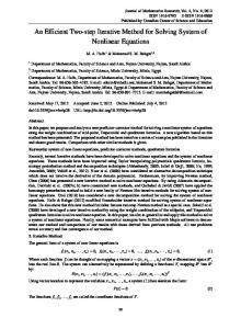
the blurred and noisy image are shown in Figures 5(a) and 5(b). The LSMR method is applied to solve this problem, while the LSQR method is used for comparison. The discrete 𝐿curve criterion is employed to choose the regularization parameter. We generate 100 instances of Gaussian white noise with noise level 𝛿 = 10−2 . For each instance, we use the discrete 𝐿-curve criterion to get the regularization parameters of LSMR and LSQR. Then, we obtain the solutions by running corresponding LSMR algorithm and LSQR algorithm. The comparison of the relative error norm is shown in Figure 2 (Example 2) and Figure 4 (Example 3). It is evident that LSMR more likely produces a better solution than LSQR. Figure 3 shows one instance of Example 2 including the true image, blurred and noisy image, and images restored by LSQR and LSMR. Similarly, Figure 5 shows one instance of Example 3. Furthermore, if we compare the optimal solution produced by LSMR and LSQR, the corresponding REN of the solution produced by LSMR is usually the smaller one. The 𝐿-curve works well for large noise level. Actually, we found that the regularization parameter obtained from the 𝐿curve is almost optimal when the level of noise is 5 × 10−2 . But the 𝐿-curve may fail or need a large number of iterations to find the corner for small noise level. Besides, we have done the comparison of LSMR and LSQR with the regularization parameter chosen by DP. LSMR method can get nearly the same REN as LSQR method, while LSQR method could be terminated somewhat sooner. The memory and computational costs of every step in LSMR are also slightly more expensive than that in LSQR [11].

5. Conclusion In this paper, we briefly introduced the IDR(𝑠) method and the LSMR method, and then we applied the IDR(𝑠) and

Abstract and Applied Analysis

7

(a)

(b)

(c)

(d)

Figure 1: (a) True image, (b) blurred and noisy image with 𝜎 = 1, (c) restored image with LSQR, and (d) restored image with IDR(1).

0.6 0.58

REN

0.56 0.54 0.52 0.5 0.48

0

10

20

30

40 50 60 70 Number of instances

80

90

100

LSQR LSMR

Figure 2: Comparison of the REN produced by LSQR and LSMR.

8

Abstract and Applied Analysis

(a)

(b)

(c)

(d)

Figure 3: (a) True image, (b) blurred and noisy image, (c) restored image with LSQR, Iter = 104, and REN = 0.5004, and (d) restored image with LSMR, Iter = 128, and REN = 0.4919. 0.46 0.44

REN

0.42 0.4 0.38 0.36 0.34 0.32

0

10

20

30

40 50 60 70 Number of instances

80

90

100

LSQR LSMR

Figure 4: Comparison of the REN produced by LSQR and LSMR.

(a)

(b)

(c)

(d)

Figure 5: (a) True image, (b) blurred and noisy image, (c) restored image with LSQR, Iter = 95, and REN = 0.3519, and (d) restored image with LSMR, Iter = 129, and REN = 0.3417.

LSMR methods to solve image deblurring problems. These methods show some superiorities when compared to the classic iterative regularization method LSQR. When DP is used to terminate the iteration, IDR(𝑠) can give a satisfactory solution with a low computational cost when 𝐴 is not very ill-condition and the noise level is low. The parameter 𝑠 has little influence on the performance of IDR(𝑠),

so we can use IDR(1) for saving storage and computational cost. LSMR performs as well as LSQR but needs more computational cost when DP is used to terminate the iteration. When the 𝐿-curve method is utilized to choose the regularization parameter, LSMR more likely produces a more accurate solution than LSQR.

Abstract and Applied Analysis

Acknowledgments This research is supported by 973 Program (2013CB329404), NSFC (61170311), Chinese Universities Specialized Research Fund for the Doctoral Program (20110185110020), and Sichuan Province Sci. & Tech. Research Project (2012GZX0080). The authors would like to express their thankfulness to the referees and the editor for their much helpful suggestions for revising this paper.

References [1] P. C. Hansen, J. G. Nagy, and D. P. O’Leary, Deblurring Images: Matries, Spectra and Filtering, Society for Industrial and Applied Mathematics, Philadelphia, Pa, USA, 2006. [2] R. J. Hanson, “A numerical method for solving Fredholm integral equations of the first kind using singular values,” SIAM Journal on Numerical Analysis, vol. 8, pp. 616–622, 1971. [3] P. C. Hansen, Rank-Deficient and Discrete Ill-Posed Problems: Numerical Aspects of Linear Inversion, Society for Industrial and Applied Mathematics, Philadelphia, Pa, USA, 1998. [4] Y. Saad, Iterative Methods for Sparse Linear Systems, Society for Industrial and Applied Mathematics, Philadelphia, Pa, USA, 2nd edition, 2003. [5] R. Plato, “Optimal algorithms for linear ill-posed problems yield regularization methods,” Numerical Functional Analysis and Optimization, vol. 11, no. 1-2, pp. 111–118, 1990. [6] P. C. Hansen, Discrete Inverse Problems: Insight and Algorithms, Society for Industrial and Applied Mathematics, Philadelphia, Pa, USA, 2010. [7] D. Calvetti, B. Lewis, and L. Reichel, “On the regularizing properties of the GMRES method,” Numerische Mathematik, vol. 91, no. 4, pp. 605–625, 2002. [8] D. Calvetti, B. Lewis, and L. Reichel, “Krylov subspace iterative methods for nonsymmetric discrete ill-posed problems in image restoration,” in Advanced Signal Processing: Algorithms, Architectures and Implementations XI, vol. 4474 of Proceedings of SPIE, pp. 224–233, The International Society for Optical Engineering, Bellingham, Wash, USA, August 2001. [9] P. Brianzi, P. Favati, O. Menchi, and F. Romani, “A framework for studying the regularizing properties of Krylov subspace methods,” Inverse Problems, vol. 22, no. 3, pp. 1007–1021, 2006. [10] P. Sonneveld and M. B. van Gijzen, “IDR(s): a family of simple and fast algorithms for solving large nonsymmetric systems of linear equations,” SIAM Journal on Scientific Computing, vol. 31, no. 2, pp. 1035–1062, 2008. [11] D. C.-L. Fong and M. Saunders, “LSMR: an iterative algorithm for sparse least-squares problems,” SIAM Journal on Scientific Computing, vol. 33, no. 5, pp. 2950–2971, 2011. [12] M. B. van Gijzen and P. Sonneveld, “An elegant IDR(s) variant that efficiently exploits bi-orthogonality properties,” Tech. Rep. 08-21, Department of Applied Mathematical Analysis, Delft University of Technology, Delft, The Netherlands, 2008. [13] V. Simoncini and D. B. Szyld, “Interpreting IDR as a PetrovGalerkin method,” SIAM Journal on Scientific Computing, vol. 32, no. 4, pp. 1898–1912, 2010. [14] M. Hanke, Conjugate Gradient Type Methods for Ill-Posed Problems, vol. 327 of Pitman Research Notes in Mathematics Series, Longman, Harlow, UK, 1995.

9 [15] T. K. Jensen and P. C. Hansen, “Iterative regularization with minimum-residual methods,” BIT, vol. 47, no. 1, pp. 103–120, 2007. [16] P. Sonneveld, “On the convergence behaviour of IDR(s),” Tech. Rep. 10-08, Department of Applied Mathematical Analysis, Delft University of Technology, Delft, The Netherlands, 2010. [17] M. Donatelli and S. Serra-Capizzano, “On the regularizing power of multigrid-type algorithms,” SIAM Journal on Scientific Computing, vol. 27, no. 6, pp. 2053–2076, 2006. [18] M. Donatelli and S. Serra-Capizzano, “Filter factor analysis of an iterative multilevel regularizing method,” Electronic Transactions on Numerical Analysis, vol. 29, pp. 163–177, 2007/08. [19] V. A. Morozov, “On the solution of functional equations by the method of regularization,” Soviet Mathematics. Doklady, vol. 7, pp. 414–417, 1966. [20] P. C. Hansen, “Analysis of discrete ill-posed problems by means of the L-curve,” SIAM Review, vol. 34, pp. 658–672, 1992. [21] G. Wahba, “Practical approximate solutions to linear operator equations when the data are noisy,” SIAM Journal on Numerical Analysis, vol. 14, no. 4, pp. 651–667, 1977. [22] I. Hnˇetynkov´a, M. Pleˇsinger, and Z. Strakoˇs, “The regularizing effect of the Golub-Kahan iterative bidiagonalization and revealing the noise level in the data,” BIT, vol. 49, no. 4, pp. 669– 696, 2009. [23] L. Reichel and G. Rodriguez, “Old and new parameter choice rules for discrete ill-posed problems,” Numerical Algorithms, vol. 63, no. 1, pp. 65–87, 2013. [24] P. C. Hansen, T. K. Jensen, and G. Rodriguez, “An adaptive pruning algorithm for the discrete L-curve criterion,” Journal of Computational and Applied Mathematics, vol. 198, no. 2, pp. 483–492, 2007. [25] P. C. Hansen, “The L-curve and its use in the numerical treatment of inverse problems,” in Computational Inverse Problems in Electrocardiology, P. Johnston, Ed., pp. 119–142, WIT Press, Southampton, Ceremonial, 2001. [26] C. R. Vogel, “Non-convergence of the L-curve regularization parameter selection method,” Inverse Problems, vol. 12, no. 4, pp. 535–547, 1996. [27] M. Hanke, “Limitations of the L-curve method in ill-posed problems,” BIT, vol. 36, no. 2, pp. 287–301, 1996. [28] D. C. L. Fong, Minimum-residual methods for sparse leastsquares using golub-kahan bidiagonalization [Ph.D. thesis], Stanford University, Stanford, Calif, USA, 2011. [29] P. C. Hansen, “Regularization tools: a Matlab package for analysis and solution of discrete ill-posed problems,” Numerical Algorithms, vol. 6, no. 1-2, pp. 1–35, 1994.

Advances in

Operations Research Hindawi Publishing Corporation http://www.hindawi.com

Volume 2014

Advances in

Decision Sciences Hindawi Publishing Corporation http://www.hindawi.com

Volume 2014

Mathematical Problems in Engineering Hindawi Publishing Corporation http://www.hindawi.com

Volume 2014

Journal of

Algebra Hindawi Publishing Corporation http://www.hindawi.com

Probability and Statistics Volume 2014

The Scientific World Journal Hindawi Publishing Corporation http://www.hindawi.com

Hindawi Publishing Corporation http://www.hindawi.com

Volume 2014

International Journal of

Differential Equations Hindawi Publishing Corporation http://www.hindawi.com

Volume 2014

Volume 2014

Submit your manuscripts at http://www.hindawi.com International Journal of

Advances in

Combinatorics Hindawi Publishing Corporation http://www.hindawi.com

Mathematical Physics Hindawi Publishing Corporation http://www.hindawi.com

Volume 2014

Journal of

Complex Analysis Hindawi Publishing Corporation http://www.hindawi.com

Volume 2014

International Journal of Mathematics and Mathematical Sciences

Journal of

Hindawi Publishing Corporation http://www.hindawi.com

Stochastic Analysis

Abstract and Applied Analysis

Hindawi Publishing Corporation http://www.hindawi.com

Hindawi Publishing Corporation http://www.hindawi.com

International Journal of

Mathematics Volume 2014

Volume 2014

Discrete Dynamics in Nature and Society Volume 2014

Volume 2014

Journal of

Journal of

Discrete Mathematics

Journal of

Volume 2014

Hindawi Publishing Corporation http://www.hindawi.com

Applied Mathematics

Journal of

Function Spaces Hindawi Publishing Corporation http://www.hindawi.com

Volume 2014

Hindawi Publishing Corporation http://www.hindawi.com

Volume 2014

Hindawi Publishing Corporation http://www.hindawi.com

Volume 2014

Optimization Hindawi Publishing Corporation http://www.hindawi.com

Volume 2014

Hindawi Publishing Corporation http://www.hindawi.com

Volume 2014