Jun 24, 2015 - mator to speed up the learning based on .... Typically, the performance and consistency ..... of the Python for Scientific Computing Conference.
Efficient Learning for Undirected Topic Models Jiatao Gu and Victor O.K. Li Department of Electrical and Electronic Engineering The University of Hong Kong {jiataogu, vli}@eee.hku.hk
arXiv:1506.07477v1 [cs.LG] 24 Jun 2015
Abstract Replicated Softmax model, a well-known undirected topic model, is powerful in extracting semantic representations of documents. Traditional learning strategies such as Contrastive Divergence are very inefficient. This paper provides a novel estimator to speed up the learning based on Noise Contrastive Estimate, extended for documents of variant lengths and weighted inputs. Experiments on two benchmarks show that the new estimator achieves great learning efficiency and high accuracy on document retrieval and classification.
1
Introduction
Topic models are powerful probabilistic graphical approaches to analyze document semantics in different applications such as document categorization and information retrieval. They are mainly constructed by directed structure like pLSA (Hofmann, 2000) and LDA (Blei et al., 2003). Accompanied by the vast developments in deep learning, several undirected topic models, such as (Salakhutdinov and Hinton, 2009; Srivastava et al., 2013), have recently been reported to achieve great improvements in efficiency and accuracy. Replicated Softmax model (RSM) (Hinton and Salakhutdinov, 2009), a kind of typical undirected topic model, is composed of a family of Restricted Boltzmann Machines (RBMs). Commonly, RSM is learned like standard RBMs using approximate methods like Contrastive Divergence (CD). However, CD is not really designed for RSM. Different from RBMs with binary input, RSM adopts softmax units to represent words, resulting in great inefficiency with sampling inside CD, especially for a large vocabulary. Yet, NLP systems usually require vocabulary sizes of tens to hundreds of thousands, thus seriously limiting its application.
Dealing with the large vocabulary size of the inputs is a serious problem in deep-learning-based NLP systems. Bengio et al. (2003) pointed this problem out when normalizing the softmax probability in the neural language model (NNLM), and Morin and Bengio (2005) solved it based on a hierarchical binary tree. A similar architecture was used in word representations like (Mnih and Hinton, 2009; Mikolov et al., 2013a). Directed tree structures cannot be applied to undirected models like RSM, but stochastic approaches can work well. For instance, Dahl et al. (2012) found that several Metropolis Hastings sampling (MH) approaches approximate the softmax distribution in CD well, although MH requires additional complexity in computation. Hyv¨arinen (2007) proposed Ratio Matching (RM) to train unnormalized models, and Dauphin and Bengio (2013) added stochastic approaches in RM to accommodate high-dimensional inputs. Recently, a new estimator Noise Contrastive Estimate (NCE) (Gutmann and Hyv¨arinen, 2010) is proposed for unnormalized models, and shows great efficiency in learning word representations such as in (Mnih and Teh, 2012; Mikolov et al., 2013b). In this paper, we propose an efficient learning strategy for RSM named α-NCE, applying NCE as the basic estimator. Different from most related efforts that use NCE for predicting single word, our method extends NCE to generate noise for documents in variant lengths. It also enables RSM to use weighted inputs to improve the modelling ability. As RSM is usually used as the first layer in many deeper undirected models like Deep Boltzmann Machines (Srivastava et al., 2013), α-NCE can be readily extended to learn them efficiently.
2
Replicated Softmax Model
RSM is a typical undirected topic model, which is based on bag-of-words (BoW) to represent documents. In general, it consists of a series of RBMs,
each of which contains variant softmax visible units but the same binary hidden units. Suppose K is the vocabulary size. For a document with D words, if the ith word in the document equals the k th word of the dictionary, a vector vi ∈ {0, 1}K is assigned, only with the k th element vik = 1. An RBM is formed by assigning a hidden state h ∈ {0, 1}H to this document V = {v1 , ..., vD }, where the energy function is: Eθ (V , h) = −hT W v ˆ − bT v ˆ − D · aT h (1) where θ = {W , b, a} P are parameters shared by all the RBMs, and v ˆ= D i=1 vi is commonly referred to as the word count vector of a document. The probability for the document V is given by: X 1 −Fθ (V ) e−Fθ (V ) e , ZD = V ZD (2) X e−Eθ (V ,h) Fθ (V ) = log Pθ (V ) =
h
where Fθ (V ) is the “free energy”, which can be analytically integrated easily, and ZD is the “partition function” for normalization, only associated with the document length D. As the hidden state and document are conditionally independent, the conditional distributions are derived: � exp WkT h + bk Pθ (vik = 1|h) = PK � (3) T k=1 exp Wk h + bk Pθ (hj = 1|V ) = σ (Wj v ˆ + D · aj )
(4)
where σ(x) = 1+e1−x . Equation (3) is the softmax units describing the multinomial distribution of the words, and Equation (4) serves as an efficient inference from words to semantic meanings, where we adopt the probabilities of each hidden unit “activated” as the topic features. 2.1
Learning Strategies for RSM
3
Efficient Learning for RSM
Unlike (Dahl et al., 2012) that retains CD, we adopted NCE as the basic learning strategy. Considering RSM is designed for documents, we further modified NCE with two novel heuristics, developing the approach “Partial Noise Uniform Contrastive Estimate” (or α-NCE for short). 3.1
Noise Contrastive Estimate
Noise Contrastive Estimate (NCE), similar to CD, is another estimator for training models with intractable partition functions. NCE solves the intractability through treating the partition function c added to θ, ZD as an additional parameter ZD which makes the likelihood computable. Yet, the model cannot be trained through ML as the likelic to hood tends to be arbitrarily large by setting ZD huge numbers. Instead, NCE learns the model in a proxy classification problem with noise samples. Given a document collection (data) {Vd }Td , and another collection (noise) {Vn }Tn with Tn = kTd , NCE distinguishes these (1+k)Td documents simply based on Bayes’ Theorem, where we assumed data samples matched by our model, indicating Pθ ' Pdata , and noise samples generated from an artificial distribution Pn . Parameters are learned by minimizing the cross-entropy function: J(θ) = −EVd ∼Pθ [log σk (X(Vd ))]
RSM is naturally learned by minimizing the negative log-likelihood function (ML) as follows: L(θ) = −EV ∼Pdata [log Pθ (V )]
consistency improve when more steps are adopted. Notwithstanding, even one Gibbs step is time consuming for RSM, since the multinomial sampling normally requires linear time computations. The “alias method” (Kronmal and Peterson Jr, 1979) speeds up multinomial sampling to constant time while linear time is required for processing the distribution. Since Pθ (V |h) changes at every iteration in CD, such methods cannot be used.
(5)
However, the gradient is intractable for the combinatorial normalization term ZD . Common strategies to overcome this intractability are MCMCbased approaches such as Contrastive Divergence (CD) (Hinton, 2002) and Persistent CD (PCD) (Tieleman, 2008), both of which require repeating Gibbs steps of h(i) ∼ Pθ (h|V (i) ) and V (i+1) ∼ Pθ (V |h(i) ) to generate model samples to approximate the gradient. Typically, the performance and
−kEVn ∼Pn [log σk−1 (−X(Vn ))]
(6)
and the gradient is derived as follows, −∇θ J(θ) =EVd ∼Pθ [σk−1 (−X)∇θ X(Vd )] −kEVn ∼Pn [σk (X)∇θ X(Vn )] where σk (x) =
1 , 1+ke−x
(7)
and the “log-ratio” is:
X(V ) = log [Pθ (V )/Pn (V )]
(8)
J(θ) can be optimized efficiently with stochastic gradient descent (SGD). Gutmann and Hyv¨arinen (2010) showed that the NCE gradient ∇θ J(θ) will reach the ML gradient when k → ∞. In practice, a larger k tends to train the model better.
3.2
Partial Noise Sampling
Different from (Mnih and Teh, 2012), which generates noise per word, RSM requires the estimator to sample the noise at the document level. An intuitive approach is to sample from the empirical distribution p˜ for D times, where � probabil� Pthe log ity is computed: log Pn (V ) = v∈V v T log p˜ . For a fixed k, Gutmann and Hyv¨arinen (2010) suggested choosing the noise close to the data for a sufficient learning result, indicating full noise might not be satisfactory. We proposed an alternative “Partial Noise Sampling (PNS)” to generate noise by replacing part of the data with sampled words. See Algorithm 1, where we fixed the Algorithm 1 Partial Noise Sampling 1: Initialize: k, α ∈ (0, 1) 2: for each Vd = {v}D ∈ {Vd }Td do 3: Set: Dr = dα · De 4: Draw: Vr = {vr }Dr ⊆ V uniformly 5: for j = 1, ..., k do (j) (j) 6: Draw: Vn = {vn }D−Dr ∼ p˜ (j) (j) 7: Vn = Vn ∪ Vr 8: end for (1) (k) 9: Bind: (Vd , Vr ), (Vn , Vr ), ..., (Vn , Vr ) 10: end for proportion of remaining words at α, named “noise level” of PNS. However, traversing all the conditions to guess the remaining words requires O(D!) computations. To avoid this, we simply bound the remaining words with the data and noise in advance and the noise log Pn (V ) is derived readily: X � T � log Pθ (Vr ) + v log p˜ (9) v∈V \Vr
where the remaining words Vr are still assumed to be described by RSM with a smaller document length. In this way, it also strengthens the robustness of RSM towards incomplete data. Sampling the noise normally requires additional computational load. Fortunately, since p˜ is fixed, sampling is efficient using the “alias method”. It also allows storing the noise for subsequent use, yielding much faster computation than CD. 3.3
Uniform Contrastive Estimate
When we initially implemented NCE for RSM, we found the document lengths terribly biased the log-ratio, resulting in bad parameters. Therefore “Uniform Contrastive Estimate (UCE)” was proposed to accommodate variant document lengths
by adding the uniform assumption: ¯ ) = D−1 log [Pθ (V )/Pn (V )] X(V
(10)
√ where√UCE adopts the uniform probabilities D Pθ and D Pn for classification to average the modelling ability at word-level. Note that D is not necessarily an integer in UCE, and allows choosing a real-valued weights on the document such as idf -weighting (Salton and McGill, 1983). Typically, it is defined as a weighting vector w, where wk = log |V ∈{Vd }:vTikd =1,vi ∈V | is multiplied to the k th word in the dictionary. Thus for a weighted input V w and corresponding length Dw , we derive: ˜ w ) = Dw−1 log [Pθ (V w )/Pn (V w )] (11) X(V � wT � P where log Pn (V w ) = log p˜ . A v w ∈V w v c w ). specific ZD w will be assigned to Pθ (V Combining PNS and UCE yields a new estimator for RSM, which we simply call α-NCE1 .
4
Experiments
4.1
Datasets and Details of Learning
We evaluated the new estimator to train RSMs on two text datasets: 20 Newsgroups and IMDB. The 20 Newsgroups2 dataset is a collection of the Usenet posts, which contains 11,345 training and 7,531 testing instances. Both the training and testing sets are labeled into 20 classes. Removing stop words as well as stemming were performed. The IMDB dataset3 is a benchmark for sentiment analysis, which consists of 100,000 movie reviews taken from IMDB. The dataset is divided into 75,000 training instances (1/3 labeled and 2/3 unlabeled) and 25,000 testing instances. Two types of labels, positive and negative, are given to show sentiment. Following (Maas et al., 2011), no stop words are removed from this dataset. For each dataset, we randomly selected 10% of the training set for validation, and the idf -weight vector is computed in advance. In addition, replacing the word count vˆ by dlog (1 + vˆ)e slightly improved the modelling performance for all models. We implemented α-NCE according to the parameter settings in (Hinton, 2010) using SGD in minibatches of size 128 and an initialized learning rate of 0.1. The number of hidden units was fixed 1
α comes from the noise level in PNS, but UCE is also the vital part of this estimator, which is absorbed in α-NCE. 2 Available at http://qwone.com/˜jason/20Newsgroups 3 Available at http://ai.stanford.edu/˜amaas/data/sentiment
at 128 for all models. Although learning the partic separately for every length D is tion function ZD nearly impossible, as in (Mnih and Teh, 2012) we c as a constant also surprisingly found freezing ZD function of D without updating never harmed but actually enhanced the performance. It is probably because the large number of free parameters c is a in RSM are forced to learn better when ZD constant. In practise, we set this constant function P b �D c = 2H · k as ZD . It can readily extend to ke learn RSM for real-valued weighted length Dw . We also implemented CD with the same settings. All the experiments were run on a single GPU GTX970 using the library Theano (Bergstra et al., 2010). To make the comparison fair, both α-NCE and CD share the same implementation. 4.2
Evaluation of Efficiency
To evaluate the efficiency in learning, we used the most frequent words as dictionaries with sizes ranging from 100 to 20, 000 for both datasets, and test the computation time both for CD of variant Gibbs steps and α-NCE of variant noise sample sizes. The comparison of the mean running
Figure 1: Comparison of running time time per minibatch is clearly shown in Figure 1, which is averaged on both datasets. Typically, α-NCE achieves 10 to 500 times speed-up compared to CD. Although both CD and α-NCE run slower when the input dimension increases, CD tends to take much more time due to the multinomial sampling at each iteration, especially when more Gibbs steps are used. In contrast, running time stays reasonable in α-NCE even if a larger noise size or a larger dimension is applied. 4.3
to estimate the log-probability per word as perplexity. However, as α-NCE learns RSM by distinguishing the data and noise from their respective features, parameters are trained more like a feature extractor than a generative model. It is not fair to use perplexity to evaluate the performance. For this reason, we evaluated the modelling performance with some indirect measures.
Evaluation of Performance
One direct measure to evaluate the modelling performance is to assess RSM as a generative model
Figure 2: Precision-Recall curves for the retrieval task on the 20 Newsgroups dataset using RSMs. For 20 Newsgroups, we trained RSMs on the training set, and reported the results on document retrieval and document classification. For retrieval, we treated the testing set as queries, and retrieved documents with the same labels in the training set by cosine-similarity. Precision-recall (P-R) curves and mean average precision (MAP) are two metrics we used for evaluation. For classification, we trained a softmax regression on the training set, and checked the accuracy on the testing set. We use this dataset to show the modelling ability of RSM with different estimators. For IMDB, the whole training set is used for learning RSMs, and an L2-regularized logistic regression is trained on the labeled training set. The error rate of sentiment classification on the testing set is reported, compared with several BoW-based baselines. We use this dataset to show the general modelling ability of RSM compared with others. We trained both α-NCE and CD, and naturally NCE (without UCE) at a fixed vocabulary size (2000 for 20 Newsgroups, and 5000 for IMDB). Posteriors of the hidden units were used as topic features. For α-NCE , we fixed noise level at 0.5 for 20 Newsgroups and 0.3 for IMDB. In comparison, we trained CD from 1 up to 5 Gibbs steps. Figure 2 and Table 1 show that a larger noise size in α-NCE achieves better modelling perfor-
(a) MAP for document retrieval
(b) Document classification accuracy
(c) Sentiment classification accuracy
Figure 3: Tracking the modelling performance with variant α using α-NCE to learn RSMs. CD is also reported as the baseline. (a) (b) are performed on 20 Newsgroups, and (c) is performed on IMDB. mance, and α-NCE greatly outperforms CD on retrieval tasks especially around large recall values. The classification results of α-NCE is also comparable or slightly better than CD. Simultaneously, it is gratifying to find that the idf -weighting inputs achieve the best results both in retrieval and classification tasks, as idf -weighting is known to extract information better than word count. In addition, naturally NCE performs poorly compared to others in Figure 2, indicating variant document lengths actually bias the learning greatly. CD 64.1%
k=1 61.8%
α-NCE k=5 k=25 63.6% 64.8%
k=25 (idf) 65.6%
Table 1: Comparison of classification accuracy on the 20 Newsgroups dataset using RSMs. Models Bag of Words (BoW) (Maas and Ng, 2010) LDA (Maas et al., 2011) LSA (Maas et al., 2011) Maas et al. (2011)’s “full” model WRRBM (Dahl et al., 2012) RSM:CD RSM:α-NCE-5 RSM:α-NCE-5 (idf)
Accuracy 86.75% 67.42% 83.96% 87.44% 87.42% 86.22% 87.09% 87.81%
Table 2: The performance of sentiment classification accuracy on the IMDB dataset using RSMs compared to other BoW-based approaches. On the other hand, Table 2 shows the performance of RSM in sentiment classification, where model combinations reported in previous efforts are not considered. It is clear that α-NCE learns RSM better than CD, and outperforms BoW and other BoW-based models4 such as LDA. The idf 4
Accurately, WRRBM uses “bag of n-grams” assumption.
weighting inputs also achieve the best performance. Note that RSM is also based on BoW, indicating α-NCE has arguably reached the limits of learning BoW-based models. In future work, RSM can be extended to more powerful undirected topic models, by considering more syntactic information such as word-order or dependency relationship in representation. α-NCE can be used to learn them efficiently and achieve better performance. 4.4
Choice of Noise Level-α
In order to decide the best noise level (α) for PNS, we learned RSMs using α-NCE with different noise levels for both word count and idf -weighting inputs on the two datasets. Figure 3 shows that α-NCE learning with partial noise (α > 0) outperforms full noise (α = 0) in most situations, and achieves better results than CD in retrieval and classification on both datasets. However, learning tends to become extremely difficult if the noise becomes too close to the data, and this explains why the performance drops rapidly when α → 1. Furthermore, curves in Figure 3 also imply the choice of α might be problem-dependent, with larger sets like IMDB requiring relatively smaller α. Nonetheless, a systematic strategy for choosing optimal α will be explored in future work. In practise, a range from 0.3 ∼ 0.5 is recommended.
5
Conclusions
We propose a novel approach α-NCE for learning undirected topic models such as RSM efficiently, allowing large vocabulary sizes. It is new a estimator based on NCE, and adapted to documents with variant lengths and weighted inputs. We learn RSMs with α-NCE on two classic benchmarks, where it achieves both efficiency in learning and accuracy in retrieval and classification tasks.
References Yoshua Bengio, R´ejean Ducharme, Pascal Vincent, and Christian Janvin. 2003. A neural probabilistic language model. The Journal of Machine Learning Research, 3:1137–1155. James Bergstra, Olivier Breuleux, Fr´ed´eric Bastien, Pascal Lamblin, Razvan Pascanu, Guillaume Desjardins, Joseph Turian, David Warde-Farley, and Yoshua Bengio. 2010. Theano: a CPU and GPU math expression compiler. In Proceedings of the Python for Scientific Computing Conference (SciPy), June. Oral Presentation. David M Blei, Andrew Y Ng, and Michael I Jordan. 2003. Latent dirichlet allocation. the Journal of machine Learning research, 3:993–1022.
Andrew L Maas, Raymond E Daly, Peter T Pham, Dan Huang, Andrew Y Ng, and Christopher Potts. 2011. Learning word vectors for sentiment analysis. In Proceedings of the 49th Annual Meeting of the Association for Computational Linguistics: Human Language Technologies-Volume 1, pages 142–150. Association for Computational Linguistics. Tomas Mikolov, Kai Chen, Greg Corrado, and Jeffrey Dean. 2013a. Efficient estimation of word representations in vector space. arXiv preprint arXiv:1301.3781. Tomas Mikolov, Ilya Sutskever, Kai Chen, Greg S Corrado, and Jeff Dean. 2013b. Distributed representations of words and phrases and their compositionality. In Advances in Neural Information Processing Systems, pages 3111–3119.
George E Dahl, Ryan P Adams, and Hugo Larochelle. 2012. Training restricted boltzmann machines on word observations. arXiv preprint arXiv:1202.5695.
Andriy Mnih and Geoffrey E Hinton. 2009. A scalable hierarchical distributed language model. In Advances in neural information processing systems, pages 1081–1088.
Yann Dauphin and Yoshua Bengio. 2013. Stochastic ratio matching of rbms for sparse high-dimensional inputs. In Advances in Neural Information Processing Systems, pages 1340–1348.
Andriy Mnih and Yee Whye Teh. 2012. A fast and simple algorithm for training neural probabilistic language models. arXiv preprint arXiv:1206.6426.
Michael Gutmann and Aapo Hyv¨arinen. 2010. Noisecontrastive estimation: A new estimation principle for unnormalized statistical models. In International Conference on Artificial Intelligence and Statistics, pages 297–304. Geoffrey E Hinton and Ruslan R Salakhutdinov. 2009. Replicated softmax: an undirected topic model. In Advances in neural information processing systems, pages 1607–1614. Geoffrey Hinton. 2002. Training products of experts by minimizing contrastive divergence. Neural computation, 14(8):1771–1800. Geoffrey Hinton. 2010. A practical guide to training restricted boltzmann machines. Momentum, 9(1):926. Thomas Hofmann. 2000. Learning the similarity of documents: An information-geometric approach to document retrieval and categorization. Aapo Hyv¨arinen. 2007. Some extensions of score matching. Computational statistics & data analysis, 51(5):2499–2512. Richard A Kronmal and Arthur V Peterson Jr. 1979. On the alias method for generating random variables from a discrete distribution. The American Statistician, 33(4):214–218. Andrew L Maas and Andrew Y Ng. 2010. A probabilistic model for semantic word vectors. In NIPS Workshop on Deep Learning and Unsupervised Feature Learning.
Frederic Morin and Yoshua Bengio. 2005. Hierarchical probabilistic neural network language model. In Proceedings of the international workshop on artificial intelligence and statistics, pages 246–252. Citeseer. Ruslan Salakhutdinov and Geoffrey Hinton. 2009. Semantic hashing. International Journal of Approximate Reasoning, 50(7):969–978. Gerard Salton and Michael J McGill. 1983. Introduction to modern information retrieval. Nitish Srivastava, Ruslan R Salakhutdinov, and Geoffrey E Hinton. 2013. Modeling documents with deep boltzmann machines. arXiv preprint arXiv:1309.6865. Tijmen Tieleman. 2008. Training restricted boltzmann machines using approximations to the likelihood gradient. In Proceedings of the 25th international conference on Machine learning, pages 1064– 1071. ACM.