Efficient Learning with a Family of Nonconvex Regularizers by ...

Efficient Learning with a Family of Nonconvex Regularizers by Redistributing Nonconvexity

arXiv:1606.03841v2 [math.OC] 20 Oct 2016

Quanming Yao QYAOAA @ CSE . UST. HK James T. Kwok JAMESK @ CSE . UST. HK Department of Computer Science and Engineering, Hong Kong University of Science and Technology, Hong Kong

Abstract

regularizers are used in the learning of matrices (Cand`es & Recht, 2009) and tensors (Liu et al., 2013).

The use of convex regularizers allow for easy optimization, though they often produce biased estimation and inferior prediction performance. Recently, nonconvex regularizers have attracted a lot of attention and outperformed convex ones. However, the resultant optimization problem is much harder. In this paper, for a large class of nonconvex regularizers, we propose to move the nonconvexity from the regularizer to the loss. The nonconvex regularizer is then transformed to a familiar convex regularizer, while the resultant loss function can still be guaranteed to be smooth. Learning with the convexified regularizer can be performed by existing efficient algorithms originally designed for convex regularizers (such as the standard proximal algorithm and Frank-Wolfe algorithm). Moreover, it can be shown that critical points of the transformed problem are also critical points of the original problem. Extensive experiments on a number of nonconvex regularization problems show that the proposed procedure is much faster than the stateof-the-art nonconvex solvers.

Traditionally, both the loss and regularizer are convex, leading to the popularity of convex optimization tools in machine learning (Boyd & Vandenberghe, 2004). Prominent examples include the proximal algorithm (Parikh & Boyd, 2013) and, more recently, the Frank-Wolfe (FW) algorithm (Jaggi, 2013). Many of them are efficient, scalable, and have sound convergence properties. However, the use of convex regularizers often produces biased estimation, and produces solutions that are not as sparse and accurate as desired (Zhang, 2010b). To alleviate this problem, a number of nonconvex regularizers have been recently proposed (Geman & Yang, 1995; Fan & Li, 2001; Cand`es et al., 2008; Zhang, 2010a; Trzasko & Manduca, 2009). They are all (i) nonsmooth at zero, which encourages a sparse solution; and (ii) concave, which places a smaller penalty than the `1 regularizer on features with large magnitudes. Empirically, they usually outperform convex regularizers.

1. Introduction In many machine learning models, the associated optimization problems are of the form min F (x) ≡ f (x) + g(x),

x∈Rd

(1)

where x is the model parameter, f is the loss and g is the regularizer. Obviously, the choice of regularizers is important and application-specific. For example, sparsity-inducing regularizers are commonly used on highdimensional data (Jacob et al., 2009); while low-rank Proceedings of the 33 rd International Conference on Machine Learning, New York, NY, USA, 2016. JMLR: W&CP volume 48. Copyright 2016 by the author(s).

However, the resulting nonconvex problem is much harder to optimize. The concave-convex procedure (Yuille & Rangarajan, 2002) is a general technique for nonconvex optimization. However, at each iteration, the subproblem can be as expensive as the original problem, and are thus slow in practice (Gong et al., 2013; Zhong & Kwok, 2014). Recently, proximal algorithms have also been extended for nonconvex regularization (Gong et al., 2013; Li & Lin, 2015). However, efficient computation of the underlying proximal operator is only possible for simple nonconvex regularizers. When the regularizer is complicated, such as the nonconvex versions of the fused lasso or overlapping group lasso regularizers, the proximal step has to be solved numerically and is again expensive. Another approach is by using the proximal average (Zhong & Kwok, 2014), which computes and averages the proximal step of each underlying regularizer separately. However, because of its approximate proximal step, convergence is usually slower than typical applications of the proximal algorithm.

Efficient Learning with a Family of Nonconvex Regularizers by Redistributing Nonconvexity

In this paper, we propose to handle nonconvex regularizers by reusing the abundant repository of efficient convex algorithms originally designed for convex regularizers. The key is to shift the nonconvexity associated with the nonconvex regularizer to the loss function, and transform the nonconvex regularizer to a familiar convex regularizer. It will be shown that every critical point of the transformed problem is also a critical point of the original problem. To illustrate the practical usefulness of this convexification scheme, we show how it can be used with the proximal algorithm for nonconvex structured sparse learning, and with the FW algorithm for matrix learning with nonconvex low-rank regularizers. As the FW algorithm has only been used on convex problems, we also propose a new FW variant that has guaranteed convergence to a critical point of the nonconvex problem. Notation: We denote vectors and matrices by lowercase and uppercase boldface letters, respectively. For a vector Pd 1 x ∈ Rd , kxkp = ( i=1 |xi |p ) p is its `p -norm. For a matrix X ∈ Rm×n (where m ≤ n without Pm loss of generality), its nuclear norm is kXk∗ = i=1 σi (X), where σi (X)’s are the singular values of X, and its qP m Pn 2 X . For two Frobenius norm is kXkF = P i=1 j=1 ij matrices X and Y , hX, Y i = i,j Xij Yij . For a smooth function f , ∇f (x) is its gradient at x. For a convex but nonsmooth f , ∂f (x) = {u : f (y) ≥ f (x) + hu, y − xi} is its subdifferential at x, and g ∈ ∂f (x) is a subgradient.

2. Shifting Nonconvexity from Regularizer to Loss In recent years, a number of nonconvex regularizers have been proposed. Examples include the Geman penalty (GP) (Geman & Yang, 1995), log-sum penalty (LSP) (Cand`es et al., 2008), minimax concave penalty (MCP) (Zhang, 2010a), Laplace penalty (Trzasko & Manduca, 2009), and smoothly clipped absolute deviation (SCAD) penalty (Fan & Li, 2001). In general, learning with nonconvex regularizers is much more difficult than learning with convex regularizers. In this section, we show how to move the nonconvex component from the nonconvex regularizers to the loss function. Existing algorithms can then be reused to learn with the convexified regularizers.

application, we consider g of the following forms. C1. g(x) =

PK

i=1

µi gi (x), where µi ≥ 0, gi (x) = κ(kAi xkp ),

(2)

and Ai is a matrix. All the popular nonconvex regularizers in Table 1 satisfy this assumption. When κ is the identity function, g(x) reduces to the convex PK regularizer i=1 µi kAi xkp . By using different Ai ’s, this becomes various structured sparsity regularizers such as group lasso (Jacob et al., 2009), fused lasso (Tibshirani et al., 2005), and graphical lasso (Jacob et al., 2009). Pd When κ is the identity C2. g(x) = i=1 κ(|xi |). function, g becomes the lasso regularizer. Pm C3. g(X) = i=1 κ(σi (X)), where X is a matrix. When κ is the identity function, g becomes the nuclear norm regularizer. 2.1. Key Idea First, consider the form of g in C1. nonconvex gi in (2) as gi (x) = g¯i (x) + κ0 kAi xkp ,

Rewrite each (3)

where κ0 = κ0 (0), and g¯i (x) = κ(kAi xkp ) − κ0 kAi xkp . Obviously, κ0 kAi xkp is convex but nonsmooth. The following shows that g¯i , though nonconvex, is concave and Lipschitz smooth. Proposition 2.1. For p ∈ (1, +∞), κ(kzkp ) − κ0 kzkp is ¯ i -Lipschitz smooth. concave and L Corollary 2.2. For p ∈ (1, +∞), (i) g¯i is concave and ¯ i -Lipschitz smooth; (ii) g can be decomposed as g(x) = L PK g¯(x) + g˘(x), where g¯(x) ≡ ¯i (x) is concave i=1 µi g PK and Lipschitz smooth, while g˘(x) ≡ κ0 i=1 µi kAi xkp is convex but nonsmooth. Problem (1) can then be rewritten as1 min f¯(x) + g˘(x), x

(4)

A2. f is L-Lipschitz smooth (i.e., k∇f (x) − ∇f (y)k2 ≤ Lkx − yk2 ), but possibly nonconvex.

where f¯(x) ≡ f (x) + g¯(x). Note that f¯ (viewed as an ¯ ¯ = L+ augmented loss) is L-Lipschitz smooth, where L PK ¯ ˘ (viewed as a convexified regularizer) i=1 µi Li ; while g is convex but possibly nonsmooth. In other words, nonconvexity is shifted from the regularizer g to the loss f , while ensuring that the augmented loss is smooth. As will be demonstrated in the following sections, this allows

Let κ be a function that is concave, non-decreasing, ρLipschitz smooth, and κ(0) = 0. Depending on the

In the sequel, a function with a bar on top (e.g., f¯) denotes that it is smooth; whereas a function with breve (e.g., g˘) denotes that it may be nonsmooth.

First, we make the following standard assumptions on (1). A1. F is bounded from below;

1

Efficient Learning with a Family of Nonconvex Regularizers by Redistributing Nonconvexity Table 1. Example nonconvex regularizers. Here, µ > 0, and θ > 1 for SCAD, and θ > 0 for others.

κ0 (α)

κ(α) µα θ+α

GP (Geman & Yang, 1995) LSP (Cand`es et al., 2008)

( MCP (Zhang, 2010a) Laplace (Trzasko & Manduca, 2009) SCAD (Fan & Li, 2001)

µ log(1 + αθ ) µα − 1 2 2 θµ

α2 2θ

( µ 0

≤ µθ α > µθ
µ α θ exp − θ

α ≤ µθ α > µθ

µ(1 − exp(− αθ ))   µα2

−α +2θµα−µ2 2(θ−1)   µ2 (1+θ) 2

α≤µ µ < α ≤ θµ α > θµ

the reuse of existing optimization algorithms originally designed for convex regularizers on these problems with nonconvex regularizers. Similar results can be obtained for the g’s in C2 and C3. Proposition 2.3. For case C2,Pg can be decomposed as d g¯(x) + g˘(x), where g¯(x) ≡ i=1 κ(|xi |) − κ0 kxk1 is concave and Lipschitz smooth, while g˘(x) ≡ κ0 kxk1 is convex and nonsmooth. Proposition 2.4. For case C3,Pg can be decomposed as m g¯(X) + g˘(X), where g¯(X) ≡ i=1 κ(σi (X)) − κ0 kXk∗ is concave and Lipschitz smooth, while g˘(X) ≡ κ0 kXk∗ is convex and nonsmooth. The following shows that the critical points of (4) are also critical points of (1). This justifies learning via the reformulation in (4). Proposition 2.5. If x∗ is a critical point of (4), it is also a critical point of (1). Recall that g¯ is concave and g˘ is convex. Hence, the nonconvex regularizer g is decomposed as a difference of convex functions (DC) (Hiriart-Urruty, 1985). Lu (2012) and Gong et al. (2013) also relied on DC decompositions of the regularizer. However, they do not utilize this in the computational procedures, and can only handle simple nonconvex regularizers. On the other hand, we use the DC decomposition to simplify the regularizers. As will be seen, while the DC decomposition of a nonconvex function is not unique, the particular one proposed here is crucial for efficient optimization. In the following, we provide concrete examples to show how the proposed convexification scheme can be used with various optimization algorithms originally designed for convex regularizers. 2.2. Usage with Proximal Algorithms In this section, we provide example applications on using the proximal algorithm for structured sparse learning.

µθ (θ+α)2 µ θ+α − αθ α

  µ

−α+θµ  θ−1



0

α≤µ µ < α ≤ θµ α > θµ

κ0

ρ

µ θ µ θ

2µ θ2 µ θ2

µ

1 θ

µ θ

µ θ2

µ

1 θ−1

We will focus on several group lasso variants, though the proposed procedure can also be used in other applications involving proximal algorithms, such as fused lasso (Tibshirani et al., 2005) and graphical lasso (Jacob et al., 2009). The proximal algorithm (Parikh & Boyd, 2013) has been commonly used for learning with convex regularizers. With a nonconvex regularizer, the underlying proximal step becomes much more challenging. It can still be solved with the concave-convex procedure or its variant sequential convex programming (SCP) (Lu, 2012). However, they are slow in general (Gong et al., 2013; Li & Lin, 2015), as will also be empirically demonstrated in Section 3. 2.2.1. N ONCONVEX S PARSE G ROUP L ASSO The feature vector x is divided into groups, and  Gj contains dimensions in x that group j contains. Let xGj i = xi if i ∈ Gj , and 0 otherwise. The (convex) sparse group lasso is formulated as (Jacob et al., 2009): min x

N X i=1

`(yi , a> i x) + λkxk1 +

K X

µj kxGj k2 ,

j=1

where {(a1 , y1 ), . . . , (aN , yN )} are the training samples, ` is a smooth loss, and K is the number of (non-overlapping) groups. For the nonconvex extension, the regularizer
becomes Pd PK g(x) = λ i=1 κ(|xi |) + j=1 µj κ kxGj k2 . Using Corollary 2.2 and Proposition 2.3, thePconvexified regK ularizer is then g˘(x) = κ0 (λkxk1 + j=1 µj kxGj k2 ). This can be easily handled by the proximal gradient algorithm in (Yuan et al., 2011). In particular, the proximal operator of g˘ can be efficiently obtained by computing
 proxµj k·k2 proxλk·k1 xGj for each group separately. As mentioned in Section 2.1, the DC decomposition is not unique. For example, we may decompose the nonconvex gi (x) = κ(kxGi k2 ) as g˘i (x) + g¯i (x), where g¯i (x) =

Efficient Learning with a Family of Nonconvex Regularizers by Redistributing Nonconvexity

− ρ2 kxGi k22 is concave and g˘i (x) = κ (kxGi k2 ) + ρ2 kxGi k22 is convex but nonsmooth. However, such a g˘i (x) cannot be easily handled by existing proximal algorithms. 2.2.2. N ONCONVEX T REE -S TRUCTURED G ROUP L ASSO In the (convex) tree-structured group lasso (Liu & Ye, 2010; Jenatton et al., 2011), dimensions in x are organized 2 as nodes in a tree, and each group PKcorresponds to a subtree. The regularizer is of the form j=1 µj kxGj k2 . the nonconvex extension, g(x) becomes
µ κ kx k , and the convexified regularizer is j G 2 j j=1 PK g˘(x) ≡ κ0 j=1 µj kxGj k2 . As shown in (Liu & Ye, 2010), its proximal step can be computed efficiently by processing all the groups once in some appropriate order. For PK

2.3. Usage with the Frank-Wolfe Algorithm The Frank-Wolfe (FW) algorithm (Jaggi, 2013), has recently been popularly used for many convex optimization problems in machine learning. In this section, we consider as an example the learning of low-rank matrices. Its optimization problem is of the form min

X∈Rm×n

f (X) + µ

m X

κ(σi (X)),

(5)

i=1

1 kPΩ (X − O)k2F , 2

(6)

where O is the observed incomplete matrix, Ω ∈ {0, 1}m×n contains indices to the observed entries in O, and [PΩ (A)]ij = Aij if Ωij = 1; and 0 otherwise. When κ is the identity function, (5) reduces to the standard nuclear norm regularizer. Using Proposition 2.4, it can be easily seen that after convexification, problem (5) can be rewritten as min

X∈Rm×n

f¯(X) + µκ0 kXk∗ ,

(7)

¯ where Pm f (X) = f (X) + g¯(X), and g¯(X) = µ i=1 (κ(σi (X)) − κ0 σi (X)). At the tth iteration of the FW algorithm, the key linear subproblem is minS:kSk∗ ≤1 hS, ∇f¯(Xt )i, where Xt is the current iterate. Its optimal solution can be easily obtained from the rankone SVD of ∇f¯(Xt ) (Jaggi, 2013). In contrast, the FW algorithm cannot be used directly on (5), as its linear subproblem then becomes 2

Though it is computationally feasible to use FW to solve (7), note that this transformed problem is nonconvex (because of f¯), and convergence of the FW algorithm has only been shown for convex problems. In the following, we propose a FW variant (Algorithm 1) for nonconvex problems of the form (5). A low-rank factorization Ut Bt Vt> of Xt is maintained throughout the iterations. As in (Zhang et al., 2012), we adopt a local optimization scheme to speed up convergence. However, as f¯ is nonconvex and the gradient of g¯ depends on the singular values of X, the method in (Zhang et al., 2012) cannot be directly used. Instead, recall that the singular values are orthogonally invariant. Given U and V (the orthogonal left and right subspaces of X), we have g¯(X) = g¯(U BV > ) = g¯(B) and kXk∗ = kU BV > k∗ = kBk∗ . Thus, (7) can be rewritten as minU,B,V s.t.

where f is the loss. For example, in matrix completion (Cand`es & Recht, 2009), f (X) =

minS:Pm hS, ∇f (Xt )i, which is difficult. Usi=1 κ(σi (S))≤1 ing other DC decompositions, such as g¯(X) = − ρ2 kXk2F Pm ρ 2 and g˘(X) = i=1 κ(σi (X)) + 2 kXkF , will not make the optimization easier. The linear subproblem in FW then becomes minS:˘g(S)≤1 hS, ∇f¯(Xt )i, which is still difficult.

Because of the lack of space, interested readers are referred to (Liu & Ye, 2010) for details.

f (U BV > ) + g¯(B) + µκ0 kBk∗ >

(8)

>

U U = I, V V = I,

where I is the identity matrix. This can be efficiently solved using the matrix optimization techniques on Grassmann manifold (Ngo & Saad, 2012). Algorithm 1 Frank-Wolfe algorithm for solving (7). Here, QR denotes the QR factorization. 1: U0 = [], V0 = []; 2: for t = 1 . . . T do 3: [ut , st , vt ] = rank1SVD(∇f¯(Xt−1 )); ¯t = QR([Ut−1 , √st ut ]); 4: U √ ¯ 5: Vt = QR([Vt−1 , st vt ]); ¯t , V¯t as warm6: obtain [Ut , Bt , Vt ] from (8), using U > start; // (Xt = Ut Bt Vt ) ˆ , Σt , Vˆ ] = SVD(Bt ); 7: [U ˆ , Vt = Vt Vˆ ; // (Xt = Ut Σt V > ) 8: Ut = Ut U t 9: end for output Xt = Ut Σt Vt> . Existing analysis for the FW algorithm are only for convex problems. The following theorem shows convergence of Algorithm 1 to a critical point of (5). Theorem 2.6. Assume that Xt 6= 0 for t ≥ 1. The {Xt } sequence generated by Algorithm 1 converges to a critical point of (5). Further speedup is possible in the special case of matrix completion problems (where f is given by (6)). Note from steps 7 and 8 of Algorithm 1 that Xt is implicitly stored as

Efficient Learning with a Family of Nonconvex Regularizers by Redistributing Nonconvexity

a low-rank factorization Ut ΣVt> . Using (6), we can obtain ∇f¯(Xt ) as (Watson, 1992)
ˆ t> , ∇f¯(Xt ) = PΩ Ut Σt Vt> − O + Ut ΣV (9) ˆ = [Σ ˆ ii ] is a diagonal matrix with Σ ˆ ii = where Σ 0 µ (κ ([Σt ]ii ) − κ0 ). Note that Ω is sparse and the rank of Xt cannot be larger than t at the tth iteration. Thus, (9) admits a “sparse plus low-rank” structure, which can be used to significantly speed up the SVD computation (Mazumder et al., 2010; Yao & Kwok, 2015). 2.4. Other Uses of the Proposed Scheme The proposed scheme can also be used to simplify and speed up other nonconvex optimization problems in machine learning. Here, we consider as an example a recent nonconvex generalization of lasso (Gong & Ye, 2015), in which the standard `1 regularizer is extended to Pd the nonconvex version g(x) = i=1 κ(|xi |). Plugging this into (1), we arrive at the problem min f (x) + µ x

d X

κ(|xi |).

(10)

i=1

Gong & Ye (2015) proposed a sophisticated algorithm (HONOR) which involves a combination of quasi-Newton and gradient descent steps. Though the algorithm is similar to OWL-QN (Andrew & Gao, 2007) and its variant mOWL-QN (Gong, 2015), the convergence analysis in (Gong, 2015) cannot be directly applied as the regularizer is nonconvex. Instead, a non-trivial extension was developed in (Gong & Ye, 2015). Here, by convexifying the nonconvex regularizer, (10) can be rewritten as min f¯(x) + µκ0 kxk1 , x

(11)

Pd where f¯(x) = f (x) + g¯(x) and g¯(x) = µ i=1 (κ(|xi |) − κ0 |xi |). It is easy to see that the convergence analysis for mOWL-QN (specifically, Propositions 4 and 5 in (Gong, 2015)) can be immediately applied, and guarantees convergence of mOWL-QN to a critical point of (11). By Proposition 2.5, this is also a critical point of (10). Moreover, as is demonstrated in previous sections, using other DC decompositions of g will not lead to the `1 regularizer in (11), and mOWL-QN can no longer be applied. Problem (10) can be solved by either (i) directly using HONOR, or (ii) using mOWL-QN on the transformed problem (11). We believe that the latter approach is computationally more efficient. Note that both HONOR and mOWL-QN rely heavily on second-order information. In (11), the Hessian depends only on f¯, as the Hessian

due to kxk1 is zero (Andrew & Gao, 2007). However, in (10), the Hessian depends on both terms in the objective, as the second-order derivative of κ is not zero in general. HONOR constructs the approximate Hessian using only information from f , and thus ignores Pd the curvature information due to i=1 κ(|xi |). Hence, optimizing (11) with mOWL-QN is potentially faster, as all the second-order information is utilized. This will be verified empirically in Section 3.4.

3. Experiments In this section, we perform experiments on using the proposed procedure with (i) proximal algorithms (Sections 3.1 and 3.2); (ii) Frank-Wolfe algorithm (Section 3.3); and (iii) comparision with HONOR (Section 3.4). 3.1. Nonconvex Sparse Group Lasso In this section, we perform experiments on the nonconvex sparse group lasso model (Section 2.2.1) d K X X 1 κ(|xi |)+µ κ(kxGj k2 ), (12) min ky −A> xk22+λ x 2 i=1 j=1

where κ(·) is the LSP regularizer in Table 1 (with θ = 0.5). The synthetic data set is generated as follows. The groundtruth parameter vector x ¯ ∈ R10000 is divided into 100 nonoverlapping groups: {1, . . . , 100}, {101, . . . , 200}, . . . , {9901, . . . , 10000}. We randomly set 75% of the groups to zero. In each nonzero group, we randomly set 25% of its features to zero, and generate the nonzero features from the standard normal distribution N (0, 1). Using 20000 samples, entries of the input matrix A ∈ R10000×20000 are generated from N (0, 1). The ground-truth output is y¯ = A> x ¯, and training set output is y = y¯ + , where  is random noise following N (0, 0.05). The proposed algorithm will be called N2C (Nonconvexto-Convex). The proximal step of the convexified regularizer is obtained as in (Yuan et al., 2011), and the nonmonotonous accelerated proximal gradient algorithm (Li & Lin, 2015) is used for optimization. It will be compared with the following state-of-the-art algorithms: 1. SCP: Sequential convex programming (Lu, 2012), in which the LSP regularizer is decomposed as in Table 1 of (Gong et al., 2013). 2. GIST (Gong et al., 2013): Since the nonconvex regularizer is not separable, the associated proximal operator has no closed-form solution. Instead, we use SCP (with warm-start) to solve it numerically. 3. GD-PAN (Zhong & Kwok, 2014): It performs gradient descent with proximal average (Bauschke

Efficient Learning with a Family of Nonconvex Regularizers by Redistributing Nonconvexity Table 2. Results on nonconvex sparse group lasso. RMSE and MABS are scaled by 10−3 , and the CPU time is in seconds. The best and comparable results (according to the pairwise t-test with 95% confidence) are highlighted.

RMSE MABS CPU time (sec)

SCP 50.6±2.0 5.7±0.2 0.84±0.14

non-accelerated GIST GD-PAN 50.6±2.0 52.3±2.0 5.7±0.2 7.1±0.4 0.92±0.12 0.94±0.22

accelerated nmAPG N2C 50.6±2.0 50.6±2.0 5.7±0.2 5.7±0.2 0.65±0.06 0.48±0.05

convex FISTA 53.8±1.7 10.6±0.3 0.79±0.14

Table 3. Results on tree-structured group lasso. The best and comparable results (according to the pairwise t-test with 95% confidence) are highlighted.

testing accuracy (%) sparsity (%) CPU time (sec)

SCP 99.6±0.9 5.5±0.4 7.1±1.6

GIST 99.6±0.9 5.7±0.4 50.0±8.1

et al., 2008) of the nonconvex regularizers. Closedform solutions for the proximal operator of each regularizer are obtained separately, and then averaged.

GD-PAN 99.6±0.9 6.9±0.4 14.2±2.6

nmAPG 99.6±0.9 5.4±0.3 3.8±0.4

N2C 99.6±0.9 5.1±0.2 1.9±0.3

FISTA 97.2±1.8 9.2±0.2 1.0±0.4

with an inexpensive proximal step. GD-PAN, on the other hand, converges to an inferior solution.

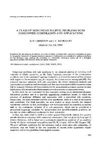
4. nmAPG (Li & Lin, 2015): This is the nonmontonous accelerated proximal algorithm. As for GIST, its proximal step does not have a closed-form solution and has to be solved numerically by SCP. 5. As a baseline, we also compare with the FISTA (Beck, 2009) algorithm, which solves the convex sparse group lasso model by removing κ from (12). We do not compare with the concave-convex procedure (Yuille & Rangarajan, 2002), which has been shown to be slow (Gong et al., 2013; Zhong & Kwok, 2014). All algorithms are implemented in Matlab. The stopping criterion is reached when the relative change in objective is smaller than 10−8 . Experiments are performed on a PC with Intel i7 CPU and 32GB memory. 50% of the data are used for training, another 25% for validation and the rest for testing. We use a fixed stepsize of η = σmax (A> A), while λ, µ in (12) are tuned by the validation set. For performance evaluation, we use the (i) testing root-mean-squared error (RMSE) on the predictions; (ii) mean absolute error of the obtained parameter x ˆ with ground-truth x, MABS = kˆ x − xk1 /10000; and (iii) CPU time. Each experiment is repeated 5 times, and the average performance reported. Results are shown in Table 2, As can be seen, all the nonconvex models obtain better RMSE and MABS than FISTA, and N2C is the fastest. Note that GD-PAN is solving an approximate problem in each iteration, and its error is slightly worse than those of the other nonconvex algorithms on this data set. Figure 1 shows convergence of the objective with time for a typical run. Clearly, N2C is the fastest, as it is based on the accelerated proximal algorithm

Figure 1. Convergence of objective vs CPU time on nonconvex sparse group lasso. FISTA is not shown as its (convex) objective is different from the others.

3.2. Nonconvex Tree-Structured Group Lasso In this section, we perform experiments on the nonconvex tree-structured group lasso model (Section 2.2.2). We use the face data set JAFFE3 , which contains 213 images with seven facial expressions: anger, disgust, fear, happy, neutral, sadness and surprise. Following (Liu & Ye, 2010), we resize each 256 × 256 image to 64 × 64. We also reuse their tree structure, which is based on pixel neighborhoods. Since our goal is only to demonstrate usefulness of the proposed convexification scheme, we focus on the binary classification problem “anger vs not-anger”. The logistic loss is used, which is more appropriate for classification. The optimization problem is min x

N X i=1

wi log 1+exp −yi ·

a> i x

K

X + µi κ (kxGi k2 ) , i=1

where κ(·) is the LSP regularizer (with θ = 0.5), 3

http://www.kasrl.org/jaffe.html

Efficient Learning with a Family of Nonconvex Regularizers by Redistributing Nonconvexity Table 4. Results on the MovieLens data sets (CPU time is in seconds). The best RMSE’s (according to the pairwise t-test with 95% confidence) are highlighted.

MovieLens-100K N2C-FW FaNCL LMaFit active

MovieLens-1M

MovieLens-10M

RMSE

rank

time

RMSE

rank

time

RMSE

rank

time

0.855±0.004 0.857±0.003 0.867±0.004 0.875±0.002

2 2 2 52