Efficient Method for Calculating the Composite Stiffness of Parabolic ...

Hindawi Publishing Corporation Mathematical Problems in Engineering Volume 2016, Article ID 5169018, 12 pages http://dx.doi.org/10.1155/2016/5169018

Research Article Efficient Method for Calculating the Composite Stiffness of Parabolic Leaf Springs with Variable Stiffness for Vehicle Rear Suspension Wen-ku Shi, Cheng Liu, Zhi-yong Chen, Wei He, and Qing-hua Zu State Key Laboratory of Automotive Simulation and Control, Jilin University, Changchun 130025, China Correspondence should be addressed to Zhi-yong Chen; chen [email protected] Received 7 October 2015; Revised 28 January 2016; Accepted 2 February 2016 Academic Editor: Reza Jazar Copyright © 2016 Wen-ku Shi et al. This is an open access article distributed under the Creative Commons Attribution License, which permits unrestricted use, distribution, and reproduction in any medium, provided the original work is properly cited. The composite stiffness of parabolic leaf springs with variable stiffness is difficult to calculate using traditional integral equations. Numerical integration or FEA may be used but will require computer-aided software and long calculation times. An efficient method for calculating the composite stiffness of parabolic leaf springs with variable stiffness is developed and evaluated to reduce the complexity of calculation and shorten the calculation time. A simplified model for double-leaf springs with variable stiffness is built, and a composite stiffness calculation method for the model is derived using displacement superposition and material deformation continuity. The proposed method can be applied on triple-leaf and multileaf springs. The accuracy of the calculation method is verified by the rig test and FEA analysis. Finally, several parameters that should be considered during the design process of springs are discussed. The rig test and FEA analytical results indicate that the calculated results are acceptable. The proposed method can provide guidance for the design and production of parabolic leaf springs with variable stiffness. The composite stiffness of the leaf spring can be calculated quickly and accurately when the basic parameters of the leaf spring are known.

1. Introduction The development of lightweight technology and energy conservation has resulted in the extensive application of leaf springs with variable stiffness on cars. Leaf springs with variable stiffness are one of the focal points in automobile leaf springs because of their advantages over traditional leaf springs [1–5]. Parabolic leaf springs are springs that have leaves with constant widths but have varying cross-sectional thicknesses along the longitudinal direction following a parabolic law. This type of leaf spring has many advantages, such as lightness of weight; mono-leaf springs have been applied in car parts. However, the reliability of multileaf springs cannot be fully guaranteed because of manufacturing limitations; therefore, this type of spring has not been widely applied on cars. Double-leaf parabolic springs with variable stiffness are the simplest form of multileaf springs with mono-leaf springs being applied in car parts. However, the reliability of multileaf springs cannot be fully guaranteed because of manufacturing limitations; therefore, this type

of spring has not been widely applied on cars. Double-leaf parabolic springs with variable stiffness are the simplest form of multileaf springs with variable stiffness and are also the final generation of this type of multileaf spring. At present, a second main spring is added under the first main spring to protect the latter for safety considerations, thus forming a triple-leaf spring with variable stiffness. Stiffness is an important design parameter for leaf springs with variable stiffness. This parameter can be calculated using three methods, namely, formula method, FEA method, and rig test. The formula and FEA methods are preferred over the rig test because of the high manpower and time requirements of the latter. The formula method is commonly used in calculating leaf spring stiffness. In [1], the main and auxiliary springs are modeled as multileaf cantilever beams, and an efficient method for calculating the nonlinear stiffness of a progressive multileaf spring is developed and evaluated. In [2], the stiffness of the leaf spring is calculated by an in-house software based on mathematical calculations using the thickness profile of the leaves. In [3], the deformations of the main

2

Mathematical Problems in Engineering

l0f

lf

l3f

l2r h1

h2

lr

2s

l1r

F2

h4

h5

h6

l1f

l2f

h3

F1

l3r

l0r

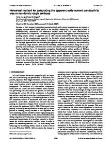
Figure 1: Two levels of parabolic leaf spring with variable stiffness.

and auxiliary springs are considered simultaneously to calculate the stiffness of the leaf spring with variable stiffness by the method of common curvature. In [4], a force model of one type of leaf spring with variable stiffness is established, and a curvature-force hybrid method for calculating the properties of such a leaf spring is developed. In [5, 6], an equation for calculating the stiffness of a leaf spring with large deflection is derived. The FEA method is also frequently used to calculate the leaf spring stiffness. In [7–9], leaf spring stiffness is calculated using the FEA method, and the result is verified by a rig test. In [10], the finite element method was used to calculate the stiffness of the parabolic leaf spring, and the effects of materials, dimensions, load, and other factors on the stiffness are discussed. In [11], an explicit nonlinear finite element geometric analysis of parabolic leaf springs under various loads is performed. The vertical stiffness, wind-up stiffness, and roll stiffness of the spring are also calculated. The FEA method is more commonly used than the formula method in the calculation of leaf spring stiffness. However, the former is more complex than the latter and requires specialized finite element software as a secondary step. Engineers who use this method should also have some work experience. By contrast, designers can easily master the formula method in calculating the stiffness of the leaf spring because it is simple and does not require special software and computer aid. Thus, deriving a stiffness calculation formula for leaf springs is significant. However, the type and size of leaf springs vary. Thus, no uniform formula can be applied to all types of leaf springs. Various equations can only fit a particular type of leaf spring. Current studies on calculating the stiffness of parabolic leaf springs with variable stiffness mostly considered the FEA method. Hence, a simple composite stiffness calculation formula should be derived for this method. The main spring bears the load alone when the load is small in parabolic leaf springs with variable stiffness in the form of main and auxiliary springs. Thereafter, the main and auxiliary springs come into contact because of the increased load. Finally, the main and auxiliary springs bear the load together when the main and auxiliary springs are under full contact. Therefore, the stiffness of the spring changes in three stages. During the first stage, the stiffness of the spring is equal to the stiffness of the main spring before the main spring and secondary springs come into contact. During the second stage, stiffness increases when the main and auxiliary springs come into contact. During the third stage, the stiffness of the spring has a composite stiffness generated by both the main and auxiliary springs when the springs are under full contact.

Changes in the stiffness of the leaf spring during stage two are nonlinear, and the stiffness is difficult to calculate. Three calculation equations are currently used [12–14] to calculate the stiffness of mono-leaf parabolic springs. However, only integral equations are available for calculating the composite stiffness of parabolic leaf spring with variable stiffness [12, 13]. However, the direct calculation of the composite stiffness of a taper-leaf spring using integral equations is quite challenging, and these equations cannot be applied during the design of a leaf spring. In this paper, a simple and practical equation for calculating the composite stiffness of parabolic leaf springs with variable stiffness is derived. The equation can be used not only for calculating the composite stiffness but also for designing such a type of leaf spring. In this paper, firstly, the leaf spring assembly model was simplified. A simple model of double-leaf parabolic spring with variable stiffness (referred to as double-leaf spring model) was considered. The difficulties in the calculation of the composite stiffness of double-leaf spring were analyzed, and the equation for calculating the composite stiffness was derived using the method of material mechanics. Thereafter, the superposition principle was used to derive the equation for triple-leaf springs. This equation can be extended to calculate the stiffness of multileaf springs. The correctness of the equation was verified by a rig test and finite element simulation. Finally, the parameters that should be considered when using the equations for leaf spring design were discussed.

2. Model of Two-Level Parabolic Leaf Spring with Variable Stiffness and Its Simplification 2.1. Leaf Spring Assembly Model. The leaf spring studied in this paper is a parabolic leaf spring with variable stiffness and unequal arm length. A triple-leaf spring model is analyzed (Figure 1). The triple-leaf spring consists of two main springs and an auxiliary spring. The stiffness of the spring is designed as a two-level variable stiffness after the requirements for a comfortable ride under different loads were considered. The first-level stiffness is the stiffness of the main spring, and the second-level stiffness is a composite stiffness determined by the stiffness of both the main and the auxiliary springs. The rear shackle is designed as an underneath shackle that makes the length of the auxiliary spring significantly less than that of the main spring because of the limited installation space

Mathematical Problems in Engineering

3

for the spring, security (leaf spring reverse bend), and vehicle performance requirements. Thus, the composite stiffness of the multileaf spring is not a simple stiffness superposition of multiple parabolic spring leaves with equal lengths. 2.2. Model Simplification. The composition of the structure of the parabolic leaf spring should be analyzed first to study its stiffness. The two main springs have the same widths and thicknesses. The primary function of the second main spring is to protect the first main spring, increasing the reliability of the leaf spring. The spring leaves contact by end, and an antifriction material is placed at the contact area. Thus, interleaf friction is not considered in the simplified model. The leaf spring force model can be simplified to a cantilever model according to the theory of material mechanics (Figure 2). The blue dashed line in Figure 2 shows an imaginary parabolic portion of the leaf spring to demonstrate the cross-sectional shape variation law of parabolic leaf springs. The triple-leaf spring model in this paper is a combination of a monoleaf (Figure 3) and a double-leaf spring model (Figure 4). The stiffness of the mono-leaf spring model can be easily obtained; thus, this study focuses on calculating the stiffness of the model shown in Figure 4. The model of a two-level leaf spring with variable stiffness will eventually develop into a double-leaf spring model (Figure 4). The highest utilization efficiency of the leaf spring material and lowest assembly weight are considered. Several assumptions are developed according to the theory of material mechanics as follows: (1) The leaf spring is generally considered a cantilever beam. A fixed constraint is applied at one of the ends. A concentration force perpendicular to the surface of the main spring is applied at the other end. (2) The unique type of force between the leaves is a vertical force. (3) The boundaries between the main and auxiliary springs should have the same curvatures and deflections. (4) The thickness of the leaves is negligible, and the main and auxiliary springs are in full contact.

3. Derivation of Equation for Calculating the Composite Stiffness for Two-Level Parabolic Leaf Springs with Variable Thickness A model for the parabolic double-leaf spring with variable stiffness (referred to as double-leaf spring model) is first examined according to the theory in Section 2. Thereafter, according to the theory of superimposition, a triple-leaf spring model was studied. Finally, the results are applied to a multileaf spring. 3.1. Challenges in Composite Stiffness Calculation. Various types of equations are used to calculate the composite stiffness of parabolic leaf springs with variable stiffness. The design part of the automobile engineering manual [7] and Spring Manual

F

Figure 2: Cantilever beam model showing the two levels of the parabolic leaf spring with variable stiffness.

F

Figure 3: Cantilever beam model of a parabolic mono-leaf spring.

F

Figure 4: Cantilever beam model of a parabolic double-leaf spring with variable stiffness.

[8] provide the following integral equation for calculating composite stiffness: 𝑥2 1 1 𝑙𝑚 = 𝑑𝑥, ∫ 𝐾 2𝜉 0 𝐸 (𝐼𝑎 (𝑥) + 𝐼𝑚 (𝑥))

(1)

where 𝐾 stands for the spring composite stiffness, 𝐸 stands for the material elastic modulus, 𝜉 is the distortion correction coefficient, 𝐼𝑎 (𝑥) is the sectional moment of inertia of the auxiliary spring, 𝐼𝑚 (𝑥) is the sectional moment of inertia of the main spring, and 𝑙𝑚 stands for half-length of the main spring. The integral equation is difficult to use in the direct calculation of the composite stiffness of the spring because of the variable cross sections of the main and auxiliary springs. Numerical integration is used to solve the problem, which cannot be performed without a computer. This study is conducted to determine whether a simple and accurate formula can be derived to calculate the composite stiffness of a parabolic leaf spring with variable stiffness. The theory of material mechanics is used to derive the equation for calculating the composite stiffness. 3.2. Derivation of Equation for Calculating the Deflection of a Mono-Leaf Spring. The deflection of the single parabolic leaf spring (mono-leaf spring) is the basis for calculating the deflection of a double-leaf spring. First, the mono-leaf spring equation is theoretically derived to obtain the equation for the deflection of any point along the leaf. The deformation of the leaf is considered when a force is applied at the end or middle part of the leaf. However, the leaf forced at the end is a special case compared with that when the leaf is forced at the

4

Mathematical Problems in Engineering l x

O

h1x

D

h1

h2

C

B

A

F

l0

s l1 l2

Figure 5: Mono-leaf spring (half-spring) with a force at its midsection.

midsection. First, the mono-leaf spring with an applied force at its midsection is considered. 3.2.1. Theoretical Derivation of Mono-Leaf Spring with an Applied Force at Its Midsection. Differential equations are established segmentally, and integration constants are obtained from boundary conditions on the basis of materialbend deformation theory. A force model of a mono-leaf spring (half-spring) with an applied force at its midsection is built and shown in Figure 5. Point 𝐷 is selected as the coordinate origin. The 𝑥-axis is located in the horizontal right, whereas the 𝑦-axis is vertically downward. 𝑓(𝑥) is the deflection of the point with a distance of 𝑥 from point 𝐷. ℎ1𝑥 is the thickness function of the parabolic part on the leaf, and ℎ1𝑥 = ℎ2 √(𝑥 + 𝑙0 )/𝑙2 . (1) Differential equations are built segmentally using material-bend deformation theory. Step 1. For CD section with bending moment 𝑀(𝑥1 ) = 𝐹𝑥1 (0 ≤ 𝑥1 ≤ 𝑙1 − 𝑙0 ) and sectional moment of inertia 𝐼1 , the deflection curve differential equation is expressed as follows: 𝐸𝐼1 𝑓1󸀠󸀠 (𝑥1 ) = 𝐹𝑥1 .

(2)

The equation is integrated once, and the double integral of 𝑥1 is as follows: 1 𝐸𝐼1 𝑓1󸀠 (𝑥1 ) = 𝐹𝑥1 2 + 𝐶1 , 2

(3)

1 𝐸𝐼1 𝑓1 (𝑥1 ) = 𝐹𝑥1 3 + 𝐶1 𝑥1 + 𝐷1 . 6

𝐸𝐼2 𝑓2󸀠󸀠 (𝑥2 ) = 𝑀 (𝑥2 ) −1/2

1/2

𝐸𝐼2 𝑓2󸀠 (𝑥2 ) = 2𝐹𝑙23/2 [(𝑥2 + 𝑙0 )

−1/2

+ 𝑙0 (𝑥2 + 𝑙0 )

]

+ 𝐶2 , 𝐸𝐼2 𝑓2 (𝑥2 ) =

4𝐹𝑙23/2

1 3/2 1/2 [ (𝑥2 + 𝑙0 ) + 𝑙0 (𝑥2 + 𝑙0 ) ] 3

(5)

+ 𝐶2 𝑥2 + 𝐷2 . Step 3. For the 𝐴𝐵 section with bending moment of 𝑀(𝑥) = 𝐹𝑥3 (𝑙2 − 𝑙0 ≤ 𝑥3 ≤ 𝑙 − 𝑙0 ) and sectional moment of inertia of 𝐼2 , the deflection curve differential equation is as follows: 𝐸𝐼2 𝑓3󸀠󸀠 (𝑥3 ) = 𝐹𝑥3

(𝑙2 − 𝑙0 ≤ 𝑥3 ≤ 𝑙 − 𝑙0 ) .

(6)

Integrating will yield the following equations: 1 𝐸𝐼2 𝑓3󸀠 (𝑥3 ) = 𝐹𝑥32 + 𝐶3 , 2 1 𝐸𝐼2 𝑓3 (𝑥3 ) = 𝐹𝑥33 + 𝐶3 𝑥3 + 𝐷3 . 6

(7)

(2) Deflection and rotation angle are determined based on the boundary conditions and continuity of deflection to solve the constants in the differential equations. Step 1. For the boundary condition in which the spring is fixed at point 𝐶 (𝑥3 = 𝑙 − 𝑙0 ), 𝑓3󸀠 (𝑙 − 𝑙0 ) = 𝑓3 (𝑙 − 𝑙0 ) = 0.

(8)

Constants 𝐶3 and 𝐷3 are calculated by (7)-(8) as follows:

Step 2. For the BC section with bending moment 𝑀(𝑥2 ) = 𝐹𝑥2 (𝑙1 − 𝑙0 ≤ 𝑥2 ≤ 𝑙2 − 𝑙0 ) and sectional moment of inertia 3 /12 = (𝑏ℎ23 /12)((𝑥2 + 𝑙0 )/𝑙2 )3/2 = 𝐼2 ((𝑥2 + 𝐼2𝑥 (𝑥) = 𝑏ℎ1𝑥 3/2 𝑙0 )/𝑙2 ) ; then the deflection curve differential equation is expressed as follows:

= 𝑙23/2 𝐹 [(𝑥2 + 𝑙0 )

Integrating will result in the following equation:

−3/2

− 𝑙0 (𝑥2 + 𝑙0 )

].

(4)

𝐶3 = −

𝐹 2 (𝑙 − 𝑙0 ) , 2

𝐹 3 𝐷3 = (𝑙 − 𝑙0 ) . 3

(9)

Step 2. The continuity of deformation at point 𝐵 (𝑥2 = 𝑥3 = 𝑙2 − 𝑙0 ) is considered: 𝑓2󸀠 (𝑙2 − 𝑙0 ) = 𝑓3󸀠 (𝑙2 − 𝑙0 ) , 𝑓2 (𝑙2 − 𝑙0 ) = 𝑓3 (𝑙2 − 𝑙0 ) .

(10)

Mathematical Problems in Engineering

5 l x O

C

D l0

h1x

B

A s

h1

h2

F

l1 l2

Figure 6: Mono-leaf spring (half-spring) with applied force at its end.

Constants 𝐶2 and 𝐷2 are calculated by (5), (7), and (10), as follows: 3 1 𝐶2 = 𝐹 (− 𝑙22 − 3𝑙0 𝑙2 + 𝑙02 ) + 𝐶3 , 2 2 (11) 13 13 2 2 𝐷2 = 𝐹 ( 𝑙2 − 3𝑙0 𝑙2 − 3𝑙0 𝑙2 + 𝑙0 ) + 𝐷3 . 3 3 Step 3. The continuity of deformation at point 𝐵 (𝑥1 = 𝑥2 = 𝑙1 − 𝑙0 ) is considered. Thus, 𝑓1󸀠 (𝑙1 − 𝑙0 ) = 𝑓2󸀠 (𝑙1 − 𝑙0 ) , 𝑓1 (𝑙1 − 𝑙0 ) = 𝑓2 (𝑙1 − 𝑙0 ) .

(12)

Constants 𝐶1 and 𝐷1 are calculated by (3), (5), and (12), as follows: 3 𝐶1 = 𝐹 [− 𝛼3 (1 − 𝛼) 𝑙22 − 3𝛼2 (𝛼 − 1) 𝑙0 𝑙2 2 1 + (𝛼3 − 1) 𝑙02 ] + 𝐶3 𝛼3 , 2 1 𝐷1 = 𝐹 [ 𝛼3 (1 − 𝛼3 ) 𝑙23 − 3𝛼3 (1 − 𝛼) 𝑙0 𝑙22 3 2

− 3𝛼 (𝛼 −

1) 𝑙02 𝑙2

(13)

(3) The deflection curve function of the 𝐶𝐷 section (0 ≤ 𝑥1 ≤ 𝑙1 − 𝑙0 ) is as follows:

󸀠 = 𝑓𝐷2

𝐷𝑚1 𝐹 , 𝐸𝐼1

𝐶𝑚1 𝐹 . 𝐸𝐼1

(15)

The deflection at point 𝑂 is as follows: 𝑓𝑂2 =

𝐹 (−𝐶𝑚1 𝑙0 + 𝐷𝑚1 ) . 𝐸𝐼1

1 1 + 𝐹 [ 𝑙3 𝛼3 + 𝛼3 (1 − 𝛼3 ) 𝑙23 ] , 3 3

(17)

defining 𝐷𝑚10 = (𝛼3 /3)[𝑙3 + (1 − 𝛼3 )𝑙23 ] and 𝐶𝑚10 = 𝛼3 [−𝑙2 /2 − (3/2)(1 − 𝛼)𝑙22 ]. Thus, the deflection at the end (𝑥 = 0) is as follows: 𝑓𝑂1 =

𝐹𝐷𝑚10 . 𝐸𝐼1

(18)

The deflection at point 𝐷 (𝑥 = 𝑙0 ) is expressed as follows: 𝑙03 /6 + 𝐷𝑚10 + 𝐶𝑚10 𝑙0 𝐹. 𝐸𝐼1

(19)

Thus, the deflection equations for a leaf with applied forces at the end and midsection are derived. These equations will be used for the calculation of the deflection of the doubleleaf spring.

(14)

where 𝐶𝑚1 = 𝐶1 /𝐹, 𝐷𝑚1 = 𝐷1 /𝐹. The deflection and the rotation angle at point 𝐷 are obtained by setting 𝑥1 to zero: 𝑓𝐷2 = 𝑓1 (𝑥2 = 0) =

1 𝑙2 3 𝐸𝐼1 𝑓 (𝑥) = 𝐹𝑥3 + 𝐹 [− 𝛼3 − (1 − 𝛼) 𝛼3 𝑙22 ] 𝑥 6 2 2

𝑓𝐷1 =

1 + (𝛼3 − 1) 𝑙03 ] + 𝐷3 𝛼3 . 3

1 𝐸𝐼1 𝑓 (𝑥1 ) = 𝐹𝑥13 + 𝐶𝑚1 𝑥1 + 𝐷𝑚1 , 6

3.2.2. Theoretical Derivation of Mono-Leaf Spring with Applied Force at Its End. A force model of a mono-leaf spring (halfspring) with an applied force at its end is shown in Figure 6. This model is a special case of the model shown in Figure 5. Thus, (14) can be used, and 𝑙0 in (14) is set to zero to obtain the deflection curve function of 𝐶𝑂 section (0 ≤ 𝑥 ≤ 𝑙1 ) as follows:

(16)

3.3. Derivation of Equation for Composite Stiffness for DoubleLeaf Spring. A force model of a double-leaf spring (halfspring) with applied force at its end is shown in Figure 7. 𝐹 and 𝐹1 represent the forces applied at the end of the main and auxiliary springs, respectively. 𝐹1󸀠 is the reaction force of 𝐹1 , and the deflection at point 𝑂 is a superposition of the deflection caused by 𝐹1󸀠 and 𝐹1 . The force 𝐹1󸀠 is initially determined using the boundary condition at point 𝐷. Thereafter, the deflection at point 𝑂 is calculated using the superposition principle of displacement. Finally, the composite stiffness of the double-leaf spring is obtained. (1) Calculation of the Force at the Contact Point. The auxiliary spring has contact with the main spring only at its end when

6

Mathematical Problems in Engineering l x

h5

F1

D

h2x

B

h4

C

A

F

h1

h2

h1x

l1

l0

l3

s

l2

Figure 7: Force model of a double-leaf spring (half-spring).

a force is applied at the end of a double-leaf spring. The force between the two leaves is transmitted through the contact point. The deflection and rotation angle between two leaves at the contact point do not remarkably vary. Thus, the contact point has two boundary conditions, namely, equal deflections and equal rotation angles. For each boundary condition, the force between the two leaves can be calculated. Step 1 (the two leaves have the same deflections at the contact point). By using (18) and (19), the deflection at point 𝐷 of the main spring caused by force 𝐹 is as follows: 𝑓𝑚𝐷1

𝑙3 /6 + 𝐷𝑚10 + 𝐶𝑚10 𝑙0 = 0 𝐹. 𝐸𝐼1

(20)

The deflection at point 𝐷 of the main spring caused by force 𝐹1󸀠 is as follows: 𝑓𝑚𝐷2 =

𝐹1 𝐷𝑚1 . 𝐸𝐼1

𝐹1 𝐷𝑎10 , 𝐸𝐼4

𝐹1𝑓 =

𝛾3 𝐷𝑎10 + 𝐷𝑚1

where 𝜔 is a weight coefficient, with a value that ranges from zero to one. (2) The Deflection at the End Point 𝑂 Is Calculated Step 1. The deflection caused by force 𝐹 is expressed as follows: 𝑓𝑂1 =

𝐹𝐷𝑚10 . 𝐸𝐼1

(26)

Step 2. The deflection caused by force 𝐹1 is expressed as follows:

𝐹.

𝑙2 /2 + 𝐶𝑚10 𝐹1𝜃 = 30 𝐹, 𝛾 𝐶𝑎10 + 𝐶𝑚10 where 𝐶𝑎10 = 𝛽3 [−(𝑙 − 𝑙0 ) /2 − (3/2)(1 − 𝛽)𝑙32 ].

𝑓𝑂2 =

𝐹1 (𝐷𝑚1 − 𝐶𝑚1 𝑙0 ) . 𝐸𝐼1

(27)

Step 3. The total deflection at point 𝑂 is defined as follows:

(23)

Step 2 (the two leaves have the same rotation angles at the contact point). The force between two leaves can be easily calculated when they have the same rotation angles at the contact point

2

(25)

(22)

where 𝐷𝑎10 = (𝛽3 𝐹/3)[(𝑙 − 𝑙0 )3 + (1 − 𝛽3 )𝑙33 ]. For 𝑓𝑚𝐷 = 𝑓𝑎𝐷, the force at the contact point because of the same deflection is as follows: (𝑙03 /6 + 𝐷𝑚10 + 𝐶𝑚10 𝑙0 )

𝐹1 = 𝜔𝐹1𝑓 + (1 − 𝜔) 𝐹1𝜃 ,

(21)

The total deflection at point 𝐷 of the main spring is as follows: 𝑓𝑚𝐷 = 𝑓𝑚𝐷1 − 𝑓𝑚𝐷2 . The deflection at point 𝐷 of the auxiliary spring caused by 𝐹1 is as follows: 𝑓𝑎𝐷 =

The deflections or rotation angles of the two springs at their contact area are not exactly the same because of the rubber between the main and auxiliary springs at their contact area. The force at the contact point is neither 𝐹1𝑓 nor 𝐹1𝜃 . The force is a combined effect of the two forces. Thus, force 𝐹1 at the contact point is assumed to be as follows:

(24)

𝑓𝑂 = 𝑓𝑂1 − 𝑓𝑂2 = ⋅ [𝜔

𝐹 {𝐷𝑚10 − (𝐷𝑚1 − 𝐶𝑚1 𝑙0 ) 𝐸𝐼1

𝑙03 /6 + 𝐷𝑚10 + 𝐶𝑚10 𝑙0 𝛾3 𝐷𝑎10 + 𝐷𝑚1

+ (1 − 𝜔)

𝐹𝜅equ 𝑙3 𝑙02 /2 + 𝐶𝑚10 ]} = , 𝛾3 𝐶𝑎10 + 𝐶𝑚10 𝐸𝐼1

(28)

Mathematical Problems in Engineering

7 l x l1 h1

h1x

l4

s

h2x

h3x

h4

h5

h7

h8

h2

F

l3 l2

Figure 8: Force model of a triple-leaf spring (half-spring).

where

Two methods are used to calculate the composite stiffness of a parabolic double-leaf spring to further refine the value range of 𝜔 in the equations. First, (30) is used to calculate directly, whereas the second approach is to use (1) and perform numerical integration to obtain the composite stiffness. The results from the two methods are compared when 𝜔 is set to different values. When 𝜔 is 0.5 to 0.7, the result error between two methods is less than 5%.

𝜅equ (𝜆, 𝜇, 𝛼, 𝛽, 𝛾) = 𝑑𝑚10 − (𝑑𝑚1 − 𝑐𝑚1 𝜇) ⋅ [𝜔

(1/6) 𝜇3 + 𝑑𝑚10 + 𝑐𝑚10 𝜇 𝛾3 𝑑𝑎10 + 𝑑𝑚1

+ (1 − 𝜔) 𝑑𝑚10 = 𝛼

3

1 + (1 − 𝛼3 ) 𝜆3

𝑐𝑚10 = −𝛼3 𝑑𝑚1 =

𝜇2 /2 + 𝑐𝑚10 ], 𝛾3 𝑐𝑎10 + 𝑐𝑚1 3

,

1 + 3 (1 − 𝛼) 𝜆2 , 2

1 1 3 (1 − 𝜇) 𝛼3 + 𝛼3 (1 − 𝛼3 ) 𝜆3 − 3𝛼3 (1 − 𝛼) 3 3

⋅ 𝜇𝜆2 − 3𝛼2 (𝛼 − 1) 𝜇2 𝜆 +

(29)

1 3 (𝛼 − 1) 𝜇3 = 𝑑𝑚10 3

1 − 3𝛼3 (1 − 𝛼) 𝜇𝜆2 − 3𝛼2 (𝛼 − 1) 𝜇2 𝜆 − 𝜇3 + 𝛼3 𝜇2 3 − 𝛼3 𝜇, 2

𝑐𝑚1 = − +

(1 − 𝜇) 3 3 𝛼 − (1 − 𝛼) 𝛼3 𝜆2 − 3 (𝛼 − 1) 𝛼2 𝜇𝜆 2 2

1 3 1 (𝛼 − 1) 𝜇2 = 𝑐𝑚10 − 3 (𝛼 − 1) 𝛼2 𝜇𝜆 − 𝜇2 2 2

𝐾𝑠 =

+ 𝛼3 𝜇. Finally, an equation for calculating the composite stiffness of a double parabolic leaf spring is obtained, as follows: 𝐾two =

𝐸𝐼1 𝐹 = . 𝑓𝑂 𝜅equ 𝑙3

3.4. Derivation of an Equation for Calculating the Composite Stiffness of Triple-Leaf and Multileaf Springs. Compared with the double-leaf spring, triple- and multileaf springs have two or more main leaves with similar lengths. A simplified model is built as discussed in Section 2.2. Thus, the equation for calculating the composite stiffness of triple- and multileaf springs can be easily derived. A force model of a tripleleaf spring (half-spring) with an applied force at its end is built and shown in Figure 8. ℎ3𝑥 stands for the thickness of the auxiliary spring at the point with a distance of 𝑥 to the parabola vertex (end point of the main spring), ℎ3𝑥 = ℎ7 √𝑥/𝑙2 . 𝑙4 stands for the length of the section with equal thickness at the end of the second main spring, 𝑙4 = 𝑙2 (ℎ7 /ℎ8 )2 . First, two main springs with different parameters are considered. The stiffness of the added main spring is expressed as follows:

(30)

𝐸𝐼7

𝑑2𝑚10 𝑙3

,

(31)

where 𝑑2𝑚10 (𝜂, 𝛼2 ) = 𝛼23 ((1 + 𝜆3 (1 − 𝛼23 ))/3), 𝛼2 = ℎ7 /ℎ8 , and 𝐼7 = (1/12)𝑏ℎ73 . The composite stiffness of a triple-leaf spring is defined as follows: 𝐾three = 𝐾two + 𝐾𝑠 =

𝐸𝐼7 𝐸𝐼1 + . 3 𝜅equ 𝑙 𝑑2𝑚10 𝑙3

(32)

8

Mathematical Problems in Engineering

The equation for multileaf spring can be derived similarly. The parameters of the multi-main springs are generally the same. Thus, the equation for the composite stiffness of a triple-leaf spring can be simplified as follows: 𝐾three =

𝐸𝐼1 𝐸𝐼1 + . 3 𝜅equ 𝑙 𝑑𝑚10 𝑙3

Hydraulic actuator

Pusher Sliding car

Leaf spring Track

(33)

By contrast, the equation for the multileaf spring is expressed as follows: 𝐾ℎ = 𝐾two + (𝑛 − 1) 𝐾𝑡 = 𝜉 [

𝐸𝐼1 (𝑛 − 1) 𝐸𝐼1 + ], 3 𝜅equ 𝑙 𝑑𝑚10 𝑙3

(34)

where 𝑛 stands for the number of the main springs and 𝜉 is a correction factor ranging from 0.92 to 0.99.

Figure 9: Experimental apparatus for measuring the stiffness of the triple-leaf spring. Table 1: Geometric parameters of a triple-leaf spring.

3.5. Calculation of Composite Stiffness of Taper-Leaf Spring with Front and Rear Halves of Unequal Lengths. All previously derived equations for composite stiffness calculation were based on half-spring models. The composite stiffness of an entire leaf spring is calculated by determining the composite stiffness at the front and rear halves (usually they are not of equal lengths at the front and rear halves of the taper-leaf spring are are not equal just as the leaf-spring studied in this paper) which should be calculated first by using the equations shown above. 𝐾𝑓 and 𝐾𝑟 represent the composite and the stiffness of the front and rear half springs of a taper-leaf spring. The composite stiffness of the entire spring can be calculated using (33): 𝐾 = (𝐾𝑓 + 𝐾𝑟 )

𝛿 (1 + 𝜁)2 , (1 + 𝛿) (1 + 𝛿𝜁2 )

(35)

where 𝛿 = 𝐾𝑓 /𝐾𝑟 , 𝜁 = 𝑙𝑓 /𝑙𝑟 . The composite stiffness of the front half spring is expressed as follows: 𝐾𝑓 =

𝐸𝐼1 𝐸𝐼1 + . 3 𝜅equ 𝑙𝑓 𝑑𝑚10 𝑙𝑓3

(36)

The composite stiffness of the rear half spring is defined as follows: 𝐾𝑟 =

𝐸𝐼1 𝐸𝐼1 + . 𝜅equ 𝑙𝑟3 𝑑𝑚10 𝑙𝑟3

(37)

This calculation method is not limited to the triple-leaf spring studied in this paper. The method can also be used for multileaf springs. 3.6. Experimental and FEA Assessments. The correctness of the theoretical formula is verified by testing the mechanical properties of a fabricated triple-leaf spring (Figure 9). The two main leaves in the triple-leaf spring have similar geometric parameters, and the front and rear halves of each leaf have the same root thicknesses and end thicknesses. The geometric parameters of the triple-leaf spring are listed in Table 1.

Length of half-spring (mm)

Front

Rear

𝑙𝑓 = 692

𝑙𝑟 = 718

Main spring Front Rear Length of parabolic portion (mm) End thickness (mm) Root thickness (mm)

𝑙2𝑓 = 633

𝑙2𝑟 = 654

Spring 60 width 𝑏 (mm) Auxiliary spring Rear Front 𝑙3𝑓 = 492

𝑙3𝑟 = 501

ℎ1 = 10.2

ℎ4 = 10.8

ℎ2 = 14.2

ℎ5 = 23.4

The leaf spring is tested on a static stiffness test rig. The test rig consists of a hydraulic actuator, a pusher used to load the spring, rail base, tested leaf spring, sliding car, and so on. Two spring eyes are fixed to the sliding cars, and these eyes can only slide along the track when the spring is loaded. The leaf spring is loaded vertically by the actuator pusher. The load is gradually increased to 24.5 kN from 0 N and then reloaded to 0 N. The loading process, which is as long as the reloading process, is 120 s long. The load and displacement during testing are recorded, and their relationship is shown in Figure 10. The experimental results show that hysteresis loss appears during the process of loading and reloading because of the friction between the main and auxiliary springs. Thus, a hysteresis loop is found in the displacement-force curve. The change trend of leaf spring stiffness with increasing load is similar to our predictions in the previous section. When the main and auxiliary springs are under full contact, the stiffness achieves a maximum and constant value. The proposed formula is derived on the basis of the condition that the main and auxiliary springs are under full contact. Thus, the formula is only suitable for calculating the stiffness of the leaf spring when the main and auxiliary springs are under full contact. The simulation, experimental, and calculated equation (30) (𝜔 = 0.6) results are shown in Table 2. The error between the calculated and experimental

Mathematical Problems in Engineering

9 Table 3: Geometric parameters of the mono-leaf spring model.

28

Spring width 𝑏 (mm) Length of half spring 𝑙 (mm) Length of parabolic portion 𝑙2 (mm) End thickness ℎ1 (mm) Root thickness ℎ2 (mm)

Force (kN)

21

14

Mono-leaf spring 80 800 720 12 25

7

Table 4: Geometric parameters of mono-leaf spring model. 0

0

45

135 90 180 Displacement (mm)

225

Figure 10: Stiffness of the triple-leaf spring.

Table 2: Comparative results. Stiffness (N/mm) Test result Simulation result Calculation result

183.8 175.6 179.8

Relative error with test result 4.5% 2.2%

results is small (within 5%). The calculated value is smaller than the experimental value because the friction between the main and auxiliary springs is neglected during equation derivation process. Thus, the equation for composite stiffness calculation derived in this paper can fully meet the needs for engineering application. Moreover, the simulation result, which is close to the calculated result, verifies the correctness of the calculation equation.

4. Attention of the Derived Equation in the Spring Design Process The correctness of the derived equation is confirmed by the results. Thus, the equation not only can be used to calculate the stiffness of existing leaf springs but also can be used in the design of a leaf spring. During the designing process, the geometric parameters of the spring leaves can be designed on the basis of the desired stiffness of the spring. However, in the actual machining process of the leaf spring, some actual dimensions of the spring leaf vary from the calculated dimensions when reliability, stress concentration, and other factors are considered. The effect of these differences on the composite stiffness value should be determined. 4.1. Root Thickness. The value of the root thickness of the leaf spring used in the formula is not equal to the one measured on a real leaf spring. This value is defined to be the vertical offset between the vertex of the parabolic leaf spring and the point in which the parabola reaches the U-bolt (ℎ in Figure 11). However, in the production of a leaf spring, the root thickness of a leaf spring is designed to be equal to the vertical offset

Length of half-spring 𝑙 (mm) Spring width 𝑏 (mm)

700 80 Main spring Auxiliary spring Length of parabolic portion (mm) 𝑙2 = 620 𝑙3 = 500 ℎ4 = 20 End thickness (mm) ℎ1 = 10 ℎ5 = 25 Root thickness (mm) ℎ2 = 8

between the vertex of the spring leaf parabola and the point in which the parabola reaches the center bolt (ℎ+Δℎ in Figure 11) considering the reliability of the U bolt and reducing the stress of the spring at the U-bolt. 4.2. Transition Region between the Isopachous and Parabolic Portions of the Leaf Spring. During the actual processing of a leaf spring, the designer tends to increase at an arc transition region at the junction to reduce the stress concentration at the junction between isopachous and parabolic portions of the leaf spring (blue area in Figure 12). The finite element simulation analytical method is used because the shape of the transition region is difficult to use to describe the function. The effect of this transition region on stiffness calculation is examined. A group of mono-leaf spring models and a group of double-leaf spring modes are used for FEA. Their geometric parameters are shown in Tables 3 and 4. Both groups of models contain a model without a transition region and a model with arc transition region. The transition region should not be too large or too small. It matches the size of the spring leaf (as shown in Table 5). Two groups of simulation results from ABAQUS are shown in Table 5. The existence of the transition region does not remarkably affect stiffness calculation, so the error of less than 2% can be neglected. 4.3. End Thickness of Auxiliary Leaf. The end thickness of an auxiliary leaf is the thickness of the uniform thickness at the end of the auxiliary leaf (ℎ4 in Figure 1). The auxiliary spring, not the main spring, generally bears only the vertical load. Thus, in the actual structure, its end thickness can be small enough to be close to zero. If a clip exists at the end of the auxiliary spring to transmit the lateral load or a rubber block to cushion stiffness mutation, the end thickness of the auxiliary spring is minimized as long as it satisfies certain needs of the lateral load and bearing reliability of the rubber block. This characteristic is also in line with the requirements of lightness of weight.

10

Mathematical Problems in Engineering Table 5: Simulation results of models with or without transition region.

Group

The radius of the transition region (mm)

Stiffness (N/mm)

Simulation results (mm) U, U2 +1.426e − 02 −4.596e + 01 −9.193e + 01 −1.379e + 02 −1.839e + 02 −2.298e + 02 −2.758e + 02 −3.218e + 02 −3.678e + 02 −4.137e + 02 −4.597e + 02

Without transition region

Mono-leaf spring

U, U2 +1.554e − 02 −4.555e + 01 −9.112e + 01 −1.367e + 02 −1.823e + 02 −2.278e + 02 −2.734e + 02 −3.190e + 02 −3.645e + 02 −4.101e + 02 −4.557e + 02

6010

U, U2 +2.779e − 03 −9.774e + 00 −1.955e + 01 −2.933e + 01 −3.910e + 01 −4.888e + 01 −5.866e + 01 −6.843e + 01 −7.821e + 01 −8.798e + 01 −9.776e + 01

Without transition region

Double-leaf spring

U, U2 +2.779e − 03 −9.750e + 00 −1.950e + 01 −2.926e + 01 −3.901e + 01 −4.876e + 01 −5.852e + 01 −6.827e + 01 −7.802e + 01 −8.777e + 01 −9.753e + 01

Main spring 2600 Auxiliary spring 500

4.4. Other Factors. Other factors, such as U-bolt preload, leaf spring arc height, and surface treatment, also affect the stiffness value. The manner in which these factors affect the stiffness is similar to traditional leaf springs with uniform thickness.

Relative error

54.38

54.86

0.88%

132.98

133.29

0.23%

5. Conclusion The conclusion is as follows: (1) An equation for calculating the composite stiffness for multileaf springs when the main and auxiliary spring

Mathematical Problems in Engineering

11

l l2

l1

h

h + Δh

U-bolts

Arc transition area

Red dotted line is the extent of leaf springs parabolic

Figure 11: Root thickness of spring leaf. l

l2

l1

Arc transition area Red dotted line is the extent of leaf springs parabolic

Figure 12: Transition region.

are under full contact is derived. The correctness of the calculation method is verified by the rig test and simulation. (2) Parameters that should be considered for designing parabolic leaf springs are discussed to provide guidance for the design and manufacture of such leaf springs.

Nomenclature 𝑙: The length of the first main spring (subscripts 𝑓 and 𝑟 indicate the front half or rear half of the spring) (see 𝑙𝑓 and 𝑙𝑟 in Figure 1) 𝑙0 : The distance between the ends of the main and auxiliary springs (subscripts 𝑓 and 𝑟 indicate the front half or rear half of the spring) (see 𝑙0𝑓 and 𝑙0𝑟 in Figure 1) 𝜇: Ratio of 𝑙0 to 𝑙 𝑙2 : The length of the parabolic portion of the first main spring (subscripts 𝑓 and 𝑟 indicate the front half or rear half of the spring) (see 𝑙2𝑓 and 𝑙2𝑟 in Figure 1) 𝜆: Ratio of 𝑙2 to 𝑙 𝑙3 : Length of the parabolic portion of the auxiliary spring (subscripts 𝑓 and 𝑟 indicate the front half or rear half of the spring) (see 𝑙3𝑓 and 𝑙3𝑟 in Figure 1)

𝑙1 :

Length of the isopachous portion of the first main spring (subscripts 𝑓 and 𝑟 indicate the front half or rear half of the spring) (see 𝑙1𝑓 and 𝑙1𝑟 in Figure 1) ℎ1 , ℎ2 , ℎ3 : Front end thickness, root thickness, and rear end thickness of the first main spring 𝛼: Ratio of ℎ1 to ℎ2 ℎ4 , ℎ5 , ℎ6 : Front end thickness, root thickness, and rear end thickness of the auxiliary spring 𝛽: Ratio of ℎ4 to ℎ3 𝛾: Ratio of ℎ1 to ℎ4 ℎ7 , ℎ8 : Root thickness and rear end thickness of the second main spring ℎ1𝑥 , ℎ2𝑥 , ℎ3𝑥 : Thickness functions of the cross section in the parabolic portion of the first main spring, second main spring, and auxiliary spring 𝐹: Force acting at the end of the leaf spring (subscripts 𝑓 and 𝑟 indicate the front half or rear half of the spring) (see 𝐹𝑓 and 𝐹𝑟 in Figure 1) 𝑠: The half-length of the isopachous portion at the spring root 𝑏: Spring width 𝜉: Distortion correction coefficient 𝐼1 : Sectional moment of inertia at the end of the first main spring; consider 𝐼1 = 𝑏ℎ13 /12 𝐼2 : Sectional moment of inertia at the root of the first main spring; consider 𝐼2 = 𝑏ℎ23 /12 𝐼3 : Sectional moment of inertia at the end of the auxiliary spring; consider 𝐼3 = 𝑏ℎ33 /12 𝐼4 : Sectional moment of inertia at the root of the auxiliary spring; consider 𝐼4 = 𝑏ℎ43 /12.

Conflict of Interests The authors declare no conflict of interests regarding the publication of this paper.

Acknowledgments The authors would like to thank the School of Automotive Engineering, Changchun, Jilin, China, and the National Natural Science Foundation of China for supporting the project (Grant no. 51205158).

References [1] S. Kim, W. Moon, and Y. Yoo, “An efficient method for calculating the nonlinear stiffness of progressive multi-leaf springs,”

12

[2]

[3]

[4]

[5]

[6]

[7]

[8]

[9]

[10]

[11]

[12] [13] [14]

Mathematical Problems in Engineering International Journal of Vehicle Design, vol. 29, no. 4, pp. 403– 422, 2002. M. Bakir, M. Siktas, and S. Atamer, “Comprehensive durability assessment of leaf springs with CAE methods,” SAE Technical Papers 2014-01-2297, 2014. R. Liu, R. Zheng, and B. Tang, “Theoretical calculations and experimental study of gradually variable rigidity leaf springs,” Automobile Technology, vol. 11, pp. 12–15, 1993. G. Hu, P. Xia, and J. Yang, “Curvature-force hybrid method for calculating properties of leaf springs with variable stiffness,” Journal of Nanjing University of Aeronautics & Astronautics, vol. 40, no. 1, pp. 46–50, 2008. T. Horibe and N. Asano, “Large deflection analysis of beams on two-parameter elastic foundation using the boundary integral equation method,” JSME International Journal Series A: Solid Mechanics and Material Engineering, vol. 44, no. 2, pp. 231–236, 2001. D. K. Roy and K. N. Saha, “Nonlinear analysis of leaf springs of functionally graded materials,” Procedia Engineering, vol. 51, pp. 538–543, 2013. G. Savaidis, L. Riebeck, and K. Feitzelmayer, “Fatigue life improvement of parabolic leaf springs,” Materials Testing, vol. 41, no. 6, pp. 234–240, 1999. M. M. Shokrieh and D. Rezaei, “Analysis and optimization of a composite leaf spring,” Composite Structures, vol. 60, no. 3, pp. 317–325, 2003. Y. S. Kong, M. Z. Omar, L. B. Chua, and S. Abdullah, “Stress behavior of a novel parabolic spring for light duty vehicle,” International Review of Mechanical Engineering, vol. 6, no. 3, pp. 617–620, 2012. M. Soner, N. Guven, A. Kanbolat, T. Erdogus, and M. K. Olguncelik, “Parabolic leaf spring design optimization considering FEA & Rig test correlation,” SAE Technical Paper 2011-012167, 2011. Y. S. Kong, M. Z. Omar, L. B. Chua, and S. Abdullah, “Explicit nonlinear finite element geometric analysis of parabolic leaf springs under various loads,” The Scientific World Journal, vol. 2013, Article ID 261926, 11 pages, 2013. W. Liu, Automotive Design, Tsinghua University Press, Beijing, China, 2001. Editorial Board, The Design Part of the Automobile Engineering Manual, People’s Communications Press, Beijing, China, 2001. Y. Zhang, H. Liu, and D. Wang, Spring Manual, Machinery Industry Press, Beijing, China, 2008.

Advances in

Operations Research Hindawi Publishing Corporation http://www.hindawi.com

Volume 2014

Advances in

Decision Sciences Hindawi Publishing Corporation http://www.hindawi.com

Volume 2014

Journal of

Applied Mathematics

Algebra

Hindawi Publishing Corporation http://www.hindawi.com

Hindawi Publishing Corporation http://www.hindawi.com

Volume 2014

Journal of

Probability and Statistics Volume 2014

The Scientific World Journal Hindawi Publishing Corporation http://www.hindawi.com

Hindawi Publishing Corporation http://www.hindawi.com

Volume 2014

International Journal of

Differential Equations Hindawi Publishing Corporation http://www.hindawi.com

Volume 2014

Volume 2014

Submit your manuscripts at http://www.hindawi.com International Journal of

Advances in

Combinatorics Hindawi Publishing Corporation http://www.hindawi.com

Mathematical Physics Hindawi Publishing Corporation http://www.hindawi.com

Volume 2014

Journal of

Complex Analysis Hindawi Publishing Corporation http://www.hindawi.com

Volume 2014

International Journal of Mathematics and Mathematical Sciences

Mathematical Problems in Engineering

Journal of

Mathematics Hindawi Publishing Corporation http://www.hindawi.com

Volume 2014

Hindawi Publishing Corporation http://www.hindawi.com

Volume 2014

Volume 2014

Hindawi Publishing Corporation http://www.hindawi.com

Volume 2014

Discrete Mathematics

Journal of

Volume 2014

Hindawi Publishing Corporation http://www.hindawi.com

Discrete Dynamics in Nature and Society

Journal of

Function Spaces Hindawi Publishing Corporation http://www.hindawi.com

Abstract and Applied Analysis

Volume 2014

Hindawi Publishing Corporation http://www.hindawi.com

Volume 2014

Hindawi Publishing Corporation http://www.hindawi.com

Volume 2014

International Journal of

Journal of

Stochastic Analysis

Optimization

Hindawi Publishing Corporation http://www.hindawi.com

Hindawi Publishing Corporation http://www.hindawi.com

Volume 2014

Volume 2014