Nov 15, 2004 - Newsletter 57, 129. 2003; available at http://psi-k.dl.ac.uk/psi-k/ newsletters.html. 9 I. Souza, N. Marzari, and D. Vanderbilt, Phys. Rev. B 65 ...
JOURNAL OF CHEMICAL PHYSICS
VOLUME 121, NUMBER 19
15 NOVEMBER 2004
An efficient method for calculating maxima of homogeneous functions of orthogonal matrices: Applications to localized occupied orbitals Joseph E. Subotnik and Yihan Shao Department of Chemistry, University of California, Berkeley, California and Chemical Sciences Division, Lawrence Berkeley National Laboratory, Berkeley, California 94720
WanZhen Liang Laboratory of Bond Selective Chemistry, University of Science and Technology of China, Hefei, Anhui 230026, People’s Republic of China
Martin Head-Gordon Department of Chemistry, University of California, Berkeley, California and Chemical Sciences Division, Lawrence Berkeley National Laboratory, Berkeley, California 94720
共Received 15 March 2004; accepted 19 July 2004兲 We present here three new algorithms 共one purely iterative and two DIIS-like 关Direct Inversion in the Iteractive Subspace兴兲 to compute maxima of homogeneous functions of orthogonal matrices. These algorithms revolve around the mathematical lemma that, given an invertible matrix A, the function f (U)⫽Tr(AU) has exactly one local 共and global兲 maximum for U special orthogonal 关i.e., UUT⫽1 and det(U)⫽1]. This is proved in the Appendix. One application of these algorithms is the computation of localized orbitals, including, for example, Boys and Edmiston-Ruedenberg 共ER兲 orbitals. The Boys orbitals are defined as the set of orthonormal orbitals which, for a given vector space of orbitals, maximize the sum of the distances between orbital centers. The ER orbitals maximize total self-interaction energy. The algorithm presented here computes Boys orbitals roughly as fast as the traditional method 共Jacobi sweeps兲, while, for large systems, it finds ER orbitals potentially much more quickly than traditional Jacobi sweeps. In fact, the required time for convergence of our algorithm scales quadratically in the region of a few hundred basis functions 共though cubicly asymptotically兲, while Jacobi sweeps for the ER orbitals traditionally scale as the number of occupied orbitals to the fifth power. As an example of the utility of the method, we provide below the ER orbitals of nitrated and nitrosated benzene, and we discuss the chemical implications. © 2004 American Institute of Physics. 关DOI: 10.1063/1.1790971兴
I. INTRODUCTION
Boys 共 1 ,..., n 兲 ⫽
Although a set of occupied molecular orbitals can be rotated among themselves and still preserve their determinant, the associated n-electron wave function,1 one cannot but help looking for some physical meaning in one electron, individual orbitals. At the very least, the choice of ground state orbitals affects one’s chemical intuition of how individual electrons behave. In a more computational context, the choice of occupied orbitals is important in local correlation calculations,2 where one wants local orbitals so one may allow only local excitations in a correlated wave function. Several sets of localized orbitals are popular today among chemists, including those commonly attributed to Boys,3– 6,16 those of Edmiston-Ruedenberg,6,16 and those of Pipek-Mezey.7 共See Ref. 7 for a brief but thorough introduction to these different sets of orbitals and the Jacobi sweep method used to calculate them.兲 Furthermore, in solid-state physics, localized orbitals have been computed as ‘‘maximally localized Wannier functions.’’ 8 –10 Thus far, most sets of localized orbitals in common practice are found by maximizing some single-valued function of the orbitals 兵 1 ,..., n 其 . For the three methods listed above and often used by chemists, these functions have the following form: 0021-9606/2004/121(19)/9220/10/$22.00
ER 共 1 ,..., n 兲 ⫽
兺i 兩 具 i兩 r兩 i 典 兩 2 , 1
兺i 具 i i兩 r 兩 i i 典 ,
PM 共 1 ,..., n 兲 ⫽
n
Numb.Atoms
i⫽1
A⫽1
兺
兺
兩 具 i兩 P A兩 i典 兩 2.
共1兲
共2兲
共3兲
共Here, P A projects a given orbital onto the space of atomic orbitals centered at atom A.兲 Note that each of these functions can be written as a homogenous function of orthogonal matrices.11 For example, in the ER case, see Eq. 共4兲 in the following section. We will revisit this point below. Though we expect our algorithm and results to be applicable to any set of localized orbitals which maximize some homogeneous function of orthogonal matrices, for the sake of concreteness, in this paper we shall focus on the ER orbitals. The defining property of the ER orbitals was first suggested by Lennard-Jones and Pople12 when the two were looking to combine orbitals of different irreducible representations of symmetric molecules and form ‘‘equivalent orbitals.’’ The authors noted that they came upon sets of orbitals that presumably maximized orbital self⫺repulsion, and thus 9220
© 2004 American Institute of Physics
Downloaded 04 Nov 2004 to 128.32.198.31. Redistribution subject to AIP license or copyright, see http://jcp.aip.org/jcp/copyright.jsp
J. Chem. Phys., Vol. 121, No. 19, 15 November 2004
Homogeneous functions of orthogonal matrices
minimized the nonclassical exchange energy. This statement is just the fact that, for any set of orthonormal vectors, Tr
冉冊
1 ⫽ r
1
1
1
(i j 兩 兩 i j) 兺i j (i j 兩 r 兩 i j)⫽ 兺i (ii 兩 r 兩 ii)⫹ 兺 r i⫽ j
is constant in any basis. Hence, when the first term 共selfrepulsion兲 is maximized, the second term 共exchange兲 is minimized. A decade later, in their paper of 1963 共Ref. 6兲, Edmiston and Ruedenberg made this construction formal 共irregardless of any symmetry兲 and motivated the use of these orbitals as localized orbitals spanning the same space as the occupied space. Of all of the localization schemes, we consider these 共the ER兲 orbitals the most natural objects because they have such a simple physical interpretation. 共A side benefit is that, unlike Boys orbitals, ER and PipekMezey orbitals preserve ⫺ separation. See Ref. 7.兲 Unfortunately, the ER orbitals are also the most computationally expensive set to compute. In their original paper, Ruedenberg and Edmiston proposed two methods for calculating the ER orbitals. 共1兲 Jacobi sweeps. Here one moves a single step by rotating in the plane spanned by any two coordinate vectors, maximizing the ER function in that two plane. One then performs this steps over all n(n⫺1)/2 pairs of coordinate vectors, a process called a sweep. Sweeps are repeated until self-consistency is reached. 共2兲 Direct minimization following the gradient of the ER function 共i.e., steepest descent兲. Declaring that Jacobi sweeps were ‘‘simpler’’ than direct minimization, Edmiston and Ruedenberg focused on the former as the primary tool for computing ER orbitals. After all, every Jacobi sweep is guaranteed to increase the ER function; furthermore, no line minimizations are required, as each step in a single sweep has an exact distance to follow. Unfortunately, though, Jacobi sweeps do not lend themselves easily to algorithms designed to improve computational efficiency. Essentially, the problem is that an efficient Jacobi sweep algorithm must save the n 4 molecular orbital integrals (i j 兩 lk) 共which is already problematic for big systems!兲, and then update these integrals after each step. If we have just done a step in the i j plane, then the most difficult integrals to update are of the form (ip 兩 qr), a process which scales as n 3 . Because a sweep contains on the order of n 2 steps, each sweep scales as n 5 . Any attempt to improve the scaling of this algorithm will require efficient computation of the integrals (i j 兩 kl). Though this should be possible once the orbitals are well-enough localized, efficient computation will depend on the extent to which these orbitals localize, and the speed of such localization. Such an algorithm would not directly take advantage of the sparsity of the atomic orbital 共AO兲 basis; furthermore, one still has n 2 steps in each sweep, making linear scaling impossible. As such, the problem seems unnecessarily difficult—if one seeks improved scaling, one really should take steps closer to the gradient. The second approach towards optimization suggested by Edmiston and Ruedenberg does exactly that–it steps directly along the gradient, doing a line minimization in the gradient direction. Because each step requires only the gradient of the
9221
ER function, the algorithm requires only the integrals (i j 兩 j j). Starting from the AO basis, this procedure scales naively as nN 4 . However, using the sparsity of the AO basis, and given initial guess orbitals that are well localized, such integrals can be generated in linear time starting from the AO integrals 共see below兲. After all, each localized electron only interacts with a bounded number of other localized electrons around it. However, there are two concerns in doing direct minimization: 共i兲 line minimizations are costly; and 共ii兲 direct minimization does not converge quickly near a stationary point. If one seeks a quickly converging direct minimization scheme, one must invoke conjugate-gradient methods. We have indeed implemented conjugate-gradient minimization over the orthogonal group 共following Edelman et al.13兲. However, even though this method is reliable and does converge to a stationary point of the ER function, we have found the need for accurate line minimizations far more costly than the alternative algorithm we present below. In this paper, we propose a third, iterative approach towards calculating the ER orbitals, one which is faster than past algorithms and which generalizes to other localized orbitals coming from homogeneous functions of orthogonal matrices. Simlarly to direct minimization, our algorithm requires only a good-starting guess and an analog of the first derivative of the function to be maximized. Most importantly, we demonstrate in this paper that our algorithm scales roughly quadratically in the number of occupied orbitals when we have n⬇100– 200, provided that our initial guess is good. 共The algorithm should scale cubicly asymptotically as n goes to infinity.兲 II. MATHEMATICAL PRELIMINARIES
In the derivations and algorithms given below, we will make reference to SO(m), which is the manifold of orthogonal matrices with determinant 1. 关Formally, U苸SO(m) if and only if UUT ⫽Id and det(U)⫽1.] We parametrize the orthogonal group 共around the identity兲 using the exponential map: U⫽e ⌬ for ⌬ antisymmetric. For U close to the identity, there is a one-to-one map between U and ⌬. In the equations below, ⌬ is always an antisymmetric matrix, and U,D苸SO(m) always. III. A BASIC ITERATIVE APPROACH TOWARDS CALCULATING THE ER ORBITALS
We are given a set of m orthonormal occupied molecular m orbitals 兵 (0) i 其 i⫽1 and we seek the 共orthonormal兲 molecular ( ) orbitals 兵 i * 其 which are maximally self-interacting. In other words, we want to maximize the ER sum,
共 1 , 2 ,..., m 兲 ⫽
兺i 共 i i兩 i i 兲 ,
where 兵 i 其 is any set of orthonormal orbitals spanning the occupied space. Expressed as a function of an orthogonal matrix, the ER function is homogeneous of degree 4:
共 U兲 ⫽
兺
i jklr
(0) (0) (0) U ji U ki U li U ri 共 (0) j k 兩l r 兲.
共4兲
Downloaded 04 Nov 2004 to 128.32.198.31. Redistribution subject to AIP license or copyright, see http://jcp.aip.org/jcp/copyright.jsp
9222
Subotnik et al.
J. Chem. Phys., Vol. 121, No. 19, 15 November 2004
We want to maximize this function for U苸SO(m), and hence compute the ER orbitals: (i * ) ⫽ 兺 j (0) j U ji . If we parametrize SO(m) by its antisymmetric generators, i.e., we write U⫽e ⌬, and differentiate with respect to ⌬ i j , we find
⌬ij
冏
⫽4 共 R i j ⫺R ji 兲 ,
共5兲
⌬⫽0
(0) (0) (0) where R ji ⫽( (0) j i 兩 i i ). In other words, the stationary points of are those orthonormal orbitals 兵 i 其 for which ( i j 兩 j j )⫽( j i 兩 i i ). Although we cannot analytically maximize 共nor find the optimal 兵 (i * ) 其 ), we can work easily with the surrogate function (0) (0) 共 U兲 ⫽ 兺 共 i (0) i 兩i i 兲 i
⫽
(0) (0) (0) 兺i j U ji共 (0) j i 兩i i 兲
⫽
兺i j R ji U ji ⫽Tr共 RT U 兲 .
As shown in the Appendix, the function 共U兲 has a unique local 共and global兲 maximum at U⫽R(RT R) ⫺1/2. If we can assume that our initial guess orbitals, 兵 (0) 其 , are ‘‘close’’ to the ER orbitals 共a point of discussion later on兲, then this suggests a basic iterative scheme to calculate the ER orbitals.
2
that, within the space of all m⫻m matrices, Rm , we walk along the surface SO(m) until we come to a matrix D( * ) for which R( * ) is symmetric. This D( * ) often represents the ER orbitals. We say above that the orbitals 兵 (i * ) 其 are ‘‘often’’ the ER orbitals, but that need not always be the case. The convergent orbitals can be maxima, minima, or saddle points of the function 共D兲—of course, D for the ER orbitals must be the 共global兲 maximum of . One can see that this is a problem as follows: when the iteration convergences, we must have lim U(k) ⫽ lim R(k) 关共 R(k) 兲 T R(k) 兴 (⫺1/2) ⫽Id, k→⬁
k→⬁
which implies that R( * ) ⫽(R( * ) ) T . Given Eq. 共5兲 for the first derivative of , 兵 (i * ) 其 must be a stationary point of . But that is all we can say about the limit orbitals 兵 (i * ) 其 , for there are no conditions on the second derivative. One more point should be made. Although it does not seem that we are analytically guaranteed that the value of will increase over the course of several iterations, i.e., that (D(1) )⭐ (D(2) )⭐¯, it is true that, for small enough steps, the value of must increase. This is a direct consequence of the proportionality
⌬ij
冏
⫽ ⌬⫽0
1 4 ⌬ij
冏
⫽R i j ⫺R ji ⌬⫽0
共which is really what ensures that stationary points of are stationary points of 兲. Hence, for a small step, U⬇Id⫹⌬,
共1兲 Start with some orthonormal set of orbitals 兵 (0) 其 which is localized and hopefully close to the ER orbitals. 共2兲 For k⭓0, construct the two-electron integrals above (k) (k) (k) R (k) ⫽( (k) ji j i 兩 i i ). 共3兲 Construct the transformation U(k⫹1) ⫽R(k) 关共 R(k) 兲 T R(k) 兴 ⫺1/2. Define D(k⫹1) ⫽D(k) •U(k⫹1) ⫽U(1) •U(2) ...U(k) •U(k⫹1) . 共4兲 Build 兵 (k⫹1) 其 as
(k⫹1) ⫽ i
(k⫹1) (k⫹1) ⫽ 兺 (0) . 兺j (k) j U ji j D ji j
共6兲
共5兲 Set k⫽k⫹1. Repeat steps 2– 4 until R(k) is sufficiently close to symmetric and the process appears to have converged. The limit orbitals 兵 (i * ) 其 should be the desired ER orbitals, with R( * ) symmetric. If we have converged after N iterations, we define D( * ) ⫽U(1) •U(2) ...U(N) and note ( ) that (i * ) ⫽ 兺 j (0) j D ji* . We will call the iterative steps defined above steps. We emphasize that at no time in the above algorithm do we ever produce a set of orbitals 兵 (k) i 其 which is not orthonormal. Alternatively, we may say that ᭙k,U(k) 苸SO(m) where m is the number of occupied orbitals. Hence, for every k, D(k) ⫽U(1) •U(2) ...U(k) is orthogonal, where D(k) is the (0) matrix expressing 兵 (k) j 其 in terms of the orbitals 兵 i 其 . 共This constraint will be relaxed in the second algorithm we propose.兲 So the geometric picture in the algorithm above is
From a certain point of view, the reason we cannot guarantee that (D(k⫹1) )⭓ (D(k) ) for large steps is because and have different second and higher derivatives. So, even though is maximized in each step, may decrease. However, we have found empirically that, if we operate not too far from a maximum/minimum, step sizes are not too big and always increases.
IV. AN ACCELERATED DIIS-LIKE ALGORITHM
The algorithm presented above, while stable, can be greatly sped up using a DIIS-like algorithm.14,15 Just as selfconsistent field 共SCF兲 theory seeks molecular orbital matrices which are orthogonal (CT SC⫽Id) and for which the corresponding Fock matrices are block diagonal, we seek m⫻m matrices 共D兲 which are orthogonal 关i.e., D苸SO(m)] and for which the corresponding R matrices are symmetric. 关Here, we again think of the columns of D as the coefficients of the ER orbitals in the original basis given to us, i.e., i ⫽ 兺 j (0) j D ji . See Eq. 共6兲.兴 For any matrix D, we define the error of D as the lack of symmetry of R共D兲, that is,
Downloaded 04 Nov 2004 to 128.32.198.31. Redistribution subject to AIP license or copyright, see http://jcp.aip.org/jcp/copyright.jsp
J. Chem. Phys., Vol. 121, No. 19, 15 November 2004
Homogeneous functions of orthogonal matrices
E i j (D)ªR i j (D)⫺R ji (D). The assumption of any DIIS-like algorithm is that, for small changes in D, the changes in the error matrix are linear. With this in mind, we implemented the following two DIIS-like procedures 共which we call DIIS-1 and DIIS-2 and which very much parallel SCF DIIS兲: 共A兲 Start with some orthonormal set of orbitals 兵 (0) 其 which is localized and hopefully close to the ER orbitals. 共B兲 For k⭓0, compute R (k) i j and calculate the error ma(k) (k) trix E (k) i j ªR i j ⫺R ji . 共C兲 Construct the DIIS B-matrix, i.e., for 1⭐i, j⭐k, we m (i) ( j) define B i j ⫽ 具 E (i) 兩 E ( j) 典 ⫽ 兺 r,s⫽1 E rs E rs . 共D兲 Set up the standard DIIS equations and solve for 兵 (c i ) 其 :
冉
B 11
B 12
B 21
B 22
]
]
B k1
B k2
⫺1
⫺1
共E兲
¯
B 1k
⫺1
¯
B 2k
⫺1 ⫺1
¯
] B kk
⫺1
⫺1
0
�
¯
Construct
an
冊冉 冊 冉 冊
c1 0 0 c2 ¯ ⫽ ¯ . 0 ck ⫺1
extrapolated
matrix
C(k⫹1)
9223
which should have the minimum error by extrapolation. This takes us off SO(m), i.e., C(k⫹1) 苸SO(m). In other words, the extrapolated orbitals are not orthogonal. We then do a generalized step, computing D(k⫹1) , which brings us back to SO(m), so we again have orthogonal orbitals. 共A generalized step maximizes the surrogate function just like the usual step, only it recognizes that the starting orbitals are not orthonormal, but rather have overlap matrix ˜S. See part 5 of the Appendix.兲 This process is iterated until convergence. In the algorithm above there are two procedures for constructing the R matrix at the extrapolated coordinates C(k) : either by (a) explicit construction 共which is slow but exact兲, or (b) by extrapolation of previous R matrices 共which is fast, but efficient only when we are working close to the identity兲. With either method, the program jumps on and off of SO(m), and converges significantly faster than pure iterations 共see below兲. With regards to the difference between DIIS-1 and DIIS-2, we expect DIIS-1 to be more broadly applicable than DII-2; i.e., DIIS-2 is faster than DIIS-1, but should presumably require a better initial guess 共as it is formally correct only near the identity兲. The question of how good an initial guess is required will be investigated in a future paper.
k ⫽ 兺 a⫽1 c a D(a) .
共F兲 At the extrapolated C(k⫹1) , construct an extrapolated R. This can be done in two ways: 共a兲 For DIIS-1: Most formally and precisely, we may define: (k⫹1) 共i兲 (k⫹1) ⫽ 兺 j (0) . i j C ji k⫹1 (k⫹1) 兩 (k⫹1) ). 共ii兲 ˜S i j ⫽( i j (k⫹1) (k⫹1) (k⫹1) ˜ i 兩 (k⫹1) (k⫹1) ). 共iii兲 R ji ⫽( j i i
共b兲 For DIIS-2: Alternatively, we may note that, to k ⫽ 兺 a⫽1 c a R (a) first order around the identity, ˜R (k⫹1) ji ji . 共G兲 Take a generalized step. 共See part 5 of the Appendix兲. More precisely, we construct ˜ (k⫹1) ⫽ 共 ˜S(k⫹1) 兲 ⫺1 R ˜ (k⫹1) 关共 R ˜ (k⫹1) 兲 T 共 ˜S(k⫹1) 兲 ⫺1 V
V. NUMERICAL PERFORMANCE A. DIIS versus Jacobi sweeps
The algorithms described above have been implemented into a development version of the Q-CHEM program.17 A simple assessment of the speed of our DIIS-like algorithm was made by comparison to the method of Jacobi sweeps in the computation of Boys’ orbitals. Results for the simple molecule benzene (C6 H6 ) are given in Table I of the supplementary material.18 Recalling that each individual DIIS step requires evaluation of just one or two R matrices, whereas Jacobi sweeps loop over all orbital pairs and updates dipole matrices, we conclude that our algorithm competes with Jacobi sweeps for convergence.
˜ (k⫹1) 兴 ⫺1/2, ⫻R ˜ (k⫹1) , and we set we define D(k⫹1) ⫽C(k⫹1) V (k⫹1) (k⫹1) ⫽ 兺 j (0) . i j D ji
共H兲 Increment k by 1 and repeat steps 共B兲–共G兲. Iterate until convergence, which is when R(k) is sufficiently symmetric and the error matrix is close to zero. 2 Here the geometric picture in Rm is as follows. Just as before, we want to find an m⫻m matrix which is both on the manifold SO(m) and for which the corresponding R matrix is symmetric. We start out on SO(m) at the identity, D(0) ⫽Idm⫻m . We next make one step and move to C(1) ⫽D(1) , which is also on SO(m). From this point on, extrapolation occurs. Given k⫹1 points on SO(m), 兵 D(0) ,D(1) ,...,D(k) 其 , we assume that is locally a quadratic function near D(k) , and 共just as in Pulay’s DIIS algorithm兲 we estimate the point C(k⫹1) , lying in the k-dimensional subspace spanned by 兵 D(k) ⫺D(0) ,D(k) ⫺D(1) ,...,D(k) ⫺D(k⫺1) 其 ,
B. DIIS versus steps
Because our algorithm was designed to compute not just Boys’ orbitals, but also more computationally expensive orbitals, we calculated the ER orbitals for benzene (C6 H6 ) with increasing basis size. The results are given in Table II of the supplementary material.18 The data in Table II demonstrates how much faster calculations become when using DIIS-like interpolations instead of pure steps. The DIIS algorithm converges in 15 steps, where the steps take on the order of 400 steps. This difference is enormous when saddle points are encountered because DIIS-like interpolations allow you to move to nearby stationary points quickly, whereas steps move slowly and cautiously 共though more reliably兲 towards new stationary points. The quick convergence of the DIIS-like routines here reflects the parabolic and well-isolated nature of the ER maximum in the case of benzene. When the be-
Downloaded 04 Nov 2004 to 128.32.198.31. Redistribution subject to AIP license or copyright, see http://jcp.aip.org/jcp/copyright.jsp
9224
J. Chem. Phys., Vol. 121, No. 19, 15 November 2004
Subotnik et al.
havior of the ER function around the maximum is not as simple, the DIIS-like algorithms can fail to converge, and one must rely on other methods 共Jacobi sweeps, conjugate gradient, or the steady, simple procedure兲 to find a maximum. 共See the application to benzene nitrosation and nitration below for such an example.兲 The saddle point encountered in these benzene calculations can be described as follows: In the smallest basis 关Slater-type orbital 共STO兲-3G兴, the ER orbitals are 共qualitatively兲 the same as the Boys’ orbitals, mixing and orbitals, forming so-called ‘‘banana’’ bonds. As the basis size grows, however, this set of orbitals becomes a saddle point of the ER function, while the true maxima of the function becomes the usual ER orbitals 共which do not mix and orbitals兲. This unusual state of affairs, where saddle points and maxima switch 共and the qualitative properties of ER orbitals change兲 with basis size, emphasizes that one must calculate second derivatives in order to be sure one has found a valid set of orbitals. C. Scaling with system size: Alkanes
The bottleneck in doing the calculations above is the evaluation of the matrix elements (i j 兩 j j). However, using the Boys’ orbitals as our initial guess, we have generated these integrals in subquadratic 共and potentially linear兲 time. We computed these integrals by first making n matrices of the form K (i) ⫽( i 兩 i), which are then transformed into (i j 兩 j j). Most naively, this computation can be done in a 共‘‘cubic’’兲 time proportional to nN 2 , if we exploit only the sparsity of the AO basis and then transform.19 However, when we exploit the locality of our guess orbitals 共and hence the sparsity of the density matrix P i ), we can form 兵 K (i) 其 in a 共‘‘linear’’兲 time proportional to N. 20 In Figs. 1共a兲 and 1共b兲, we show the CPU time required for the computation of the ER orbitals of alkanes of increasing size 共in a STO-3G basis兲 using the two 共‘‘cubic’’ and ‘‘linear-scaling’’兲 algorithms mentioned above. Note the difference in time scale. For each algorithm, we break down the CPU time into the time needed to 共a兲 gather the AO integrals, 共b兲 digest the integrals into K (i) , and 共c兲 perform the linear algebra and manipulations required by our algorithm. This last component 共for manipulations and linear algebra兲 has not been optimized. These graphs show that the time for the ‘‘cubic’’ algorithm is dominated by the digestion of the relevant AO integrals into K (i) , and this time grows cubicly and prohibitively. For the ‘‘linear-scaling’’ algorithm, by contrast, the integrals are generated in linear time 共as expected兲. Furthermore, the digestion of the integrals into K (i) is subquadratic and should become linear asymptotically. The only problematic component of the linear-scaling algorithms is that the time required for the linear algebra and memory manipulation appears to grow cubicly, though with a small prefactor. As stated above, this code has not been optimized and improvements can be made by cleaning up the interfaces between different blocks of our own code and the way we manipulate memory storage. Notwithstanding this optimization, however, we do expect the diagonalization of RRT and the inversion of ˜S to scale cubicly with a relatively
FIG. 1. 共a兲 The CPU times 共seconds兲 required in the calculation of ER orbitals of alkanes of increasing size. The AO basis is STO-3G. Here, the ‘‘cubic’’ algorithm was employed to generate the integrals (i j 兩 j j) from the AO integrals, see text. Note the change in time between this 共a兲 and 共b兲. The dominant effect by far in this graph is digestion, which scales cubicly. For each point on this graph 共i.e., for every alkane兲, exactly seven DIIS-2 iterations were required for convergence 共which implies that DIIS-2 converges exactly as well for all alkanes of different sizes兲. 共b兲 The CPU times 共seconds兲 required in the calculation of ER orbitals of alkanes of increasing size. The AO basis is STO-3G. Here, the ‘‘linear-scaling’’ algorithm was employed to generate the integrals (i j 兩 j j) from the AO integrals, see text. Note the change in time between 共b兲 and 共a兲. Also, note that for systems larger than C50H102 , the linear algebra and memory manipulation of the algorithm require more CPU time than the integral formation and digestion. 关Again, as in 共a兲, for each point on this graph, exactly seven DIIS-2 iterations were required for convergence.兴
large prefactor. For larger and larger systems, these effects must dominate and will need to be addressed to find a truly asymptotically quadratic 共or better兲 algorithm. Perhaps in the future, the sparsity RRT will allow better than cubic diagonalization, and given that ˜S is usually close to the identity, a power series for inversion will suffice. For the moment, however, for the sizes of molecules treated today by quantum mechanics, the linear-scaling DIIS-like algorithms presented here are a big advance in the computation of ER orbitals. VI. A CHEMICAL APPLICATION: NITRATION AND NITROSATION OF BENZENE
The highly different reactivities of nitronium (NO⫹ 2 ) and nitrosonium (NO⫹ ) 23 toward benzene have been investi-
Downloaded 04 Nov 2004 to 128.32.198.31. Redistribution subject to AIP license or copyright, see http://jcp.aip.org/jcp/copyright.jsp
J. Chem. Phys., Vol. 121, No. 19, 15 November 2004
FIG. 2. 共a兲 Nuclear geometry of benzene-NO⫹ , over which is plotted a three-dimensional spatial representation of a delocalized donor-acceptor ER orbital. The orbital shown is one of three equivalent 共symmetrically related兲 orbitals. This structure was optimized with N-O vertically aligned over the center of the benzene ring. Perpendicular distance from N to benzene is 2.16 Å. 共b兲 Two-dimensional contour plot of the delocalized donor-acceptor ER orbital in benzene-NO⫹ . The plane of the contour is perpendicular to the benzene plane, cutting across the midpoints of carbon-carbon bonds 共rather than through any carbon nucleus兲.
gated from a theoretical perspective by Gwaltney et al.21 There has also been a recent comprehensive density22 The exfunctional theory 共DFT兲 study on benzene-NO⫹ 2 . perimental observation that must be explained is that NO⫹ forms a stable complex with benzene, but NO⫹ 2 does not. adds directly and rapidly to benzene to form a 共Instead, NO⫹ 2 adduct兲. The canonical explanation of the benzene-NO⫹ bonding is that the orbitals of benzene mix with the * orbitals of NO⫹ 关here we conceive NO⫹ as vertically aligned over the benzene plane–see Fig. 2共a兲兴. One wonders why NO⫹ 2 is incapable of forming such a bond, given the similar electronic properties of the two 共e.g., the two species have very similar ionization potentials in the gas phase兲? Gwaltney et al. mapped out the potential energy surfaces of both benzene-NO⫹ and benzene-NO⫹ 2 and argued that the different reactivities could be explained by the presence of different stationary points 共which would be intermediates in a reaction pathway兲. These findings matched well with conclusions based upon the application of Marcus-Hush theory. Since localized orbitals might qualitatively explain the differences in stability between benzene-NO⫹ and benzene-
Homogeneous functions of orthogonal matrices
9225
FIG. 3. 共a兲 Nuclear geometry of benzene-NO⫹ 2 , over which is plotted a three-dimensional spatial representation of the one 共unique兲 delocalized donor-acceptor ER orbital. This structure was established by placing NO⫹ 2 horizontally over the benzene ring and optimizing. The geometry here corresponds to structure 1 in the paper by Olah 共Ref. 22兲. The distance from the nitrogen atom to the benzene plane is 3.1 Å. 共b兲 Two-dimensional contour plot of the delocalized donor-acceptor ER orbital in benzene-NO⫹ 2 . The plane of the contour is perpendicular to both the benzene plane and O-N-O⫹ , passing directly through two carbon nuclei of benzene and the nitrogen nucleus of NO⫹ 2 .
NO⫹ 2 , we computed the localized 共ER兲 orbitals of these complexes using the algorithms described in the previous sections. For benzene-NO⫹ , the nuclear geometry was fixed by placing the nitrogen and oxygen atoms directly above the center of the benzene plane, and then minimizing the energy of the complex using restricted DFT with the B3LYP functional, leading to the geometry shown in Fig. 2共a兲. For the sake of convenience, we will identify the benzene plane with ⫹ the xy plane. For benzene-NO⫹ 2 , the linear cation (NO2 ) was initially placed horizontally above the benzene plane 共with nitrogen above the center of the benzene ring, and the oxygen atoms above carbon nuclei in benzene兲; subsequently, the restricted B3LYP energy was minimized leading to the geometry shown in Fig. 3共a兲.24 共This geometry corresponds to structure 1 in the paper by Olah and co-workers兲22 We shall call the plane, which incorporates the NO⫹ 2 molecule and is perpendicular to the benzene plane, the yz plane. Although the geometries of benzene-NO⫹ and benzene-NO⫹ 2 are not directly comparable in Figs. 2共a兲 and 3共a兲 共i.e., NO⫹
Downloaded 04 Nov 2004 to 128.32.198.31. Redistribution subject to AIP license or copyright, see http://jcp.aip.org/jcp/copyright.jsp
9226
Subotnik et al.
J. Chem. Phys., Vol. 121, No. 19, 15 November 2004
is vertically aligned while NO⫹ 2 is horizontally aligned over the benzene plane兲 in both cases one expects donation of electrons from benzene to the nearby cation, resulting in a stable complex. In the case of benzene-NO⫹ , five ER orbitals are distributed tightly over the NO⫹ cation, exactly as expected by a simple count of electrons. In addition, three equivalent delocalized donor-acceptor ER orbitals connect the nitrogen atom of NO⫹ to the benzene ring. These orbitals are mixtures of localized orbitals belonging to benzene with unoccupied orbitals belonging to the nitrogen atom of NO⫹ . A contour map of one delocalized ER orbital 共in the xz plane兲 is shown in Fig. 2共b兲. The shape of this delocalized ER orbital shows charge transfer, whereby benzene shares electronic density with the cation NO⫹ . In the case of benzene-NO⫹ 2 , the ER orbitals look quite different. For this geometry, only one delocalized ER orbital is spread out over both benzene and NO⫹ 2 . A threedimensional representation of this orbital is given in Fig. 3共a兲 and a two-dimensional contour map is given in Fig. 3共b兲. 共The contour map is in the xz plane.兲 This unique donoracceptor ER orbital is formed by the mixing of a localized orbital of benzene with an unoccupied orbital 共with * character兲 of NO⫹ 2 . Aside from this donor-acceptor orbital, the other two localized orbitals of benzene are unable to mix with an unoccupied orbital of NO⫹ 2 because of geometric concerns: the problem is that the x* -LUMO 共LUMO— lowest unoccupied molecular orbital兲 of NO⫹ 2 changes the sign of its phase across the yz plane. As such, only one localized orbital of benzene 共with density on the x⬍0 region兲 can mix constructively with NO⫹ 2 unoccupied orbitals. The second and third localized orbitals of benzene have density on both sides of the x⫽0 plane and, therefore, cannot mix constructively with the unoccupied orbitals of NO⫹ 2 . This example demonstrates the utility of localized orbitals, whereby conditions of symmetry can be simplified 共i.e., the symmetric properties of the canonical MOs are more cumbersome兲. Accordingly, the essential lesson drawn from these ER orbitals is that, unlike NO⫹ , NO⫹ 2 simply does not have the correct geometry 共and symmetry兲 to form a stable complex with benzene, provided that the nitrogen atom be over the center of the benzene ring. Hence, it is not surprising that unconstrained minimization breaks symmetry, bends the NO⫹ 2 cation 共as charge is transferred to it兲, and moves it horizontally from a position above the center of the benzene ring to a position above the edge of the benzene ring. For completeness, in Fig. 4 we show the donor-acceptor ER orbital of benzene-NO⫹ 2 in this more stable geometry. Here, exactly one localized orbital of benzene mixes strongly with one unoccupied orbital of NO⫹ 2 , creating a stationary complex. Even though this structure is energetically favorable compared to the geometry of Fig. 3共a兲, we note that this geometry, like Fig. 3共a兲, is also a saddle point of the energy function 共rather than a minimum兲.22,25 Thus, this structure is also unlikely to be experimentally observed; most likely, it evolves quickly into the adduct of NO⫹ 2 on benzene. In summary, we conclude that, unlike NO⫹ , NO⫹ 2 does not form a stable complex because first, basic geometric
FIG. 4. ER-localized donor-acceptor orbital for benzene-NO⫹ 2 , in which the NO⫹ 2 cation is bent and is situated above the edge of the benzene ring, over a carbon-carbon bond. This structure is the MP2-optimized structure discussed in Ref. 21. The interaction here is stronger than the interaction in Fig. 3共a兲 because symmetry here allows a strong mixing of one localized orbital of benzene with an unoccupied orbital of NO⫹ 2 . The distance from the nitrogen atom to the benzene plane is 2.17 Å.
factors push the cation to the side of the benzene ring while, second, more subtle features of the potential energy surface push benzene-NO⫹ 2 towards the adduct structure, preventing a complex above the benzene edge from being energetically stable. VII. DISCUSSION
Though the methods presented here can be powerful tools for solving homogeneous equations of orthogonal matrices, specifically those designed to compute localized orbitals, several caveats need to be explicitly stated. A first and obvious problem faced by our algorithms is the problem of invertibility of the R matrices. For the ER function, R ER i j ⫽(i j 兩 j j), while for the Boys function, ⫽ i 兩 r 兩 i • i 兩 r兩 j 典 . Stationary points occur when R is R Boys 具 典 具 ij symmetric, and each step requires inversion of RRT . As such, there are obvious difficulties when R becomes singular. Any possible physical significance of singular R matrices is unclear and certainly is specific to the function being maximized. As a rule of thumb, we have had no problems with R singularity when working with the ER function. However, the Boys’ function is apparently less well behaved, as, for example, R becomes singular when localizing the SCF orbitals of 共geometrically optimized兲 decane, C10H22 . Again, we are unaware of any physical significance behind this singularity. Second, we repeat that our fast algorithms do converge to saddle points just as they converge to maxima. This demands that one check second derivatives to confirm that one is indeed at a maxima. Of course, one need not compute all of the eigenvalues of the second-derivative matrix. Several techniques exist 共such as those of Davidson26,27兲 to compute the smallest or largest eigenvalue of a symmetric matrix; such techniques will be incorporated in future implementations of these algorithms. Even with such a test to conclude the algorithm, future work should seek to quickly find paths to the basin of the maxima directly, without passing through saddle points. Once there, we may successfully turn on the
Downloaded 04 Nov 2004 to 128.32.198.31. Redistribution subject to AIP license or copyright, see http://jcp.aip.org/jcp/copyright.jsp
J. Chem. Phys., Vol. 121, No. 19, 15 November 2004
algorithms presented in this paper. In the examples given, we have relied on the 共cheaply computed兲 Boys localized orbitals as our initial guess. But, as demonstrated above, these orbitals can correspond to a saddle point of the ER function, creating the ineffecient effect of forcing us to a saddle point, from which we must then jump off. Perhaps a few conjugate gradient steps may do the trick. However, we expect that any future algorithm designed to quickly find the basin of a maxima must rely on second-derivative information. In the case of the ER function, these derivatives involve terms with matrix elements ( jk 兩 ii) and (i j 兩 ik). We speculate that these should not be that much more computationally expensive to compute than the terms from the first derivative, (i j 兩 j j). Though the coulomb-like integral ( jk 兩 ii) will be harder to bound, each localized orbital still does interact with only a bounded number of other localized orbitals. Third, and potentially most difficult, the DIIS-like algorithms presented above fail when the error near the maximum does not change linearly with small changes in the choice of orbitals. This occurs when the function is quartic near the maximum or, in practice, when the Hessian has a small eigenvalue in the region surrounding the purported maximum. For example, in the case of nitrated benzene, the ER function has one rather flat direction in the vicinity of the maximum. This fact complicated our procedure for calculating ER orbitals, as we were forced to use a combination of quicker, but more dangerous, DIIS-like steps and steadier, but slower, steps. Finally, throughout this paper, we have not considered the case of multiple local maxima, which is a reality at the very least when the nuclear geometry, as in the case of benzene, has certain symmetries. However, such a global problem has no easy solution and was not investigated here. Notwithstanding these liabilities, the algorithms presented here do potentially allow the calculation of ER orbitals for larger systems than those treated before, provided that the defining function is well behaved near its maximum. Given that the matrix elements (i j 兩 j j) are computed in a timely, linear fashion, we expect that this algorithm will be very useful in helping to search for the best local picture of electronic orbitals. And as the benzene nitration/nitrosation example above demonstrates, such localized orbitals can help us understand the quantum chemistry of bonding.
Homogeneous functions of orthogonal matrices
als, as well as other orbitals coming from homogeneous functions of orthogonal matrices, provided that we start from a good initial guess. It remains to integrate this algorithm with a good global optimizer, which can take one to the basin of the ER function’s maximum in an optimal amount of time. If a decent initial guess can be made, though, this algorithm 共or a derivative thereof兲 will likely find use as computational chemists seek to find and exploit localized orbitals.
ACKNOWLEDGMENTS
We thank Greg Beran, Anthony Dutoi, and Luis Seijo for useful discussions. J.E.S. was supported by the Fannie and John Hertz Foundation. Additionally, this work was supported by the Department of Energy through the Computational Nanosciences program. M.H.G. is a part owner of Q-CHEM.
APPENDIX 1. A mathematical lemma
In this paper, we use the following lemma: Given an invertible matrix A and a function f :SO(n)→R defined by f 共 U兲 ⫽
A i j U ji ⫽Tr共 AU兲 兺 i, j
then f has one unique local 共and global兲 maximum. Proof: Let U be an orthogonal matrix for which f is maximal, and consider, for O orthogonal, g(O)⫽Tr(AUO) ⫽Tr(BO)⫽ 兺 i, j B i j O ji , where B⫽AU. 2. Stationary points
We think of the orthogonal group as generated by the vector space of antisymmetric matrices (O⫽e ⌬), and differentiate in those directions:
冉 冊冏 g ⌬ pq
⫽ ⌬⫽0
⫽
O
ji Bij 兺 ⌬ pq i, j
冏
⌬⫽0
B i j 共 ␦ j p ␦ iq ⫺ ␦ jq ␦ ip 兲 兺 i, j
VIII. SUMMARY
Localized orbitals are and will continue to be an essential tool in the future of quantum chemistry, as on the one hand, they lend themselves to chemical interpretation and, on the other hand, they may be helpful in facilitating more efficient calculations. For instance, the choice of localized occupied orbitals, upon which virutal excitations are made, is necessarily a crucial ingredient in any recipe for post Hartree-Fock local-correlation wave functions. If they can be computed quickly, the ER orbitals may well be used as building blocks in future local-correlation work because, by minimizing 兺 i⫽ j (i j 兩 i j), we expect the two-electron integrals generated from these orbitals to be very sparse, helping to speed up computation. With that in mind, this paper has presented algorithms which very quickly compute the ER orbit-
9227
⫽B qp ⫺B pq ⫽
兺i A qi U ip ⫺A pi U iq .
So g is stationary whenever AU⫽(AU) T , i.e., AU is symmetric. ˜ where N To find U, we write A in polar form:30 A⫽NU ˜ is a positive definite Hermitian form and U is unitary. If we ˜ U, also unitary, then we require write V⫽U B⫽NV⫽ 共 NV兲 T ⫽VT N⫽BT .
共A1兲
To find V, we diagonalize N⫽C ⌳C where ⌳ is positive along the diagonal and C is unitary. We rewrite Eq. 共A1兲 as CT ⌳CV⫽VT CT ⌳C, or ⌳⫽W⌳W, where W⫽CVT CT is unitary. Let W⫽(w i j ) and T
Downloaded 04 Nov 2004 to 128.32.198.31. Redistribution subject to AIP license or copyright, see http://jcp.aip.org/jcp/copyright.jsp
9228
Subotnik et al.
J. Chem. Phys., Vol. 121, No. 19, 15 November 2004
W ⫽ 2
and
⌳⫽
冉
冉
t 11
t 12
t 21
t 22
]
]
t n1
t n2
1
0
0
2
]
]
0
0
¯
t 1n
¯
t 2n
¯
t nn
�
¯
]
0
¯
0
�
]
¯
n
冊
冊
.
Given that ᭙i, i ⬎0, this can only be satisfied if, ᭙i,t ii ⫽1, i.e., W2 ⫽Id. Accordingly W must be symmetric, which implies V is symmetric 共and still orthogonal兲. Finally, because V is symmetric, Eq. 共A1兲 implies that NV⫽VN, which in turn implies that N and V can be simultaneously diagonalized: N⫽DT ⌳N D and V⫽DT ⌳V D where ⌳V is all ⫾1 on the diagonal. To solve for U, we recall V ˜ U hence U⫽U ˜ T DT ⌳V D. This can be put in terms of A, ⫽U ˜ and N⫽ 冑AAT 共here using the polarization formulas A⫽NU ˜ ⫽N⫺1 A we mean the postive square root兲. Then, U T ⫺1/2 ⫽(AA ) A. It follows that D ⌳V D.
U⫽A 共 AA 兲
T
This formula gives all of the stationary values of g, which include the maximal values of f . D here is the matrix of eigenvalues of N, not necessarily unique. As it turns out, only one of these points is a maximum.
3. Maxima
Again expanding an arbitary unitary matrix O around the identity, it follows that, to second order,
2 O wi ⌬ pq ⌬ rs
冏
1 ⫽ 关 ␦ wp 共 ␦ qr ␦ is ⫺ ␦ qs ␦ ir 兲 ⫹ ␦ qi 共 ␦ wr ␦ ps 2 ⌬⫽0 ⫺ ␦ ws ␦ pr 兲 ⫺ ␦ wq 共 ␦ pr ␦ is ⫺ ␦ ps ␦ ir 兲 ⫺ ␦ pi 共 ␦ wr ␦ qs ⫺ ␦ ws ␦ qr 兲兴 .
Hence,
2g ⌬ pq ⌬ rs
冏
⫽ ⌬⫽0
兺 i, j
B iw
M rs ⌬⫽0
⫽M pr B sp M rs ⫹M sq B qr M rs ⫺M ps B rp M rs ⫺M rq B sq M rs ⫽Tr共 MT BMT ⫹MBM⫺MT BM⫺MBMT 兲
It is easy to see that
1 ⫹ 2 ⫹¯⫹ n ⫽t 11 1 ⫹t 22 2 ⫹¯⫹t nn n .
T ⫺1/2
冏
⫽Tr关 B共 MT MT ⫹MM⫺MT M⫺MMT 兲兴 .
Because t ii ⫽ 兺 j w i j w ji and 兺 j w 2i j ⫽1, it follows by 兩 t ii 兩 ⬍1. Moreover, Tr(⌳) Cauchy-Schwarz that ⫽Tr(W⌳W)⫽Tr(W2 ⌳) says that
T
2g
兺 M pq ⌬ pq ⌬ rs pqrs
2 O wi ⌬ pq ⌬ rs
1 ⫽ 关共 B sp ⫹B ps 兲 ␦ qr ⫹ 共 B qr ⫹B rq 兲 ␦ ps 2 ⫺ 共 B rp ⫹B pr 兲 ␦ qs ⫺ 共 B sq ⫹B qs 兲 ␦ pr 兴 ⫽ 共 B sp ␦ qr ⫹B qr ␦ ps ⫺B rp ␦ qs ⫺B sq ␦ pr 兲 . To check for negative definiteness, note that
Y ⫽MT MT ⫹MM⫺MT M⫺MMT ⫽⫺ 共 M⫺MT 兲 • 共 M⫺MT 兲 T is a nonpositive matrix. Because we are interested only in antisymmetric M 共the tangent space of the orthogonal group兲, it follows Y⫽0. Hence, Y is negative definite. We claim the sum above is negative ᭙M iff B is positive definite. Recall from the preceding section, B⫽NV⫽DT ⌳D where now we define ⌳⫽⌳N ⌳V . To check, we first suppose that B⫽DT ⌳D is positive definite. Then Tr共 BY兲 ⫽Tr共 DT ⌳⫹ DY兲 ⫽Tr共 ⌳⫹ DYDT 兲 ⬍0, since DYDT is still negative definite. Conversely, choose M ⫽DT SD and Y⫽4DT S2 D where, S ␣ ⫽ ␦ ␣ i ␦  j ⫺ ␦ ␣ j ␦  i , 共 S 2 兲 ␣ ⫽⫺ ␦ ␣ i ␦  i ⫺ ␦ ␣ j ␦  j .
Then the requirement 1 4
Tr共 BY兲 ⫽Tr共 DT ⌳S2 D兲 ⫽Tr共 ⌳S2 兲 ⫽⫺⌳ ii ⫺⌳ j j ⬍0
demands that ᭙i, j ⌳ ii ⫹⌳ j j ⬎0. So we can have at most one negative eigenvalue of ⌳. But for SO(n), we further demand that ⌳ 11⌳ 22 ...⌳ nn ⬎0 so, in fact, ᭙i,⌳ ii ⬎0. B must be positive definite. Hence, we conclude that the only orthogonal matrix U for which f is maximal is when B⫽DT ⌳D⫽DT ⌳N ⌳V D is positive definite. Since ⌳N is positive definite, this requires ⌳V ⫽Id, and it follows that the only maximum is at U⫽AT 共 AAT 兲 ⫺1/2, where here we take the positive square root.
䊐.
4. Carlson-Keller corollary
One should note that the theorem above provides immediate 共re兲proof of the Carlson-Keller theorem,28 that S⫺1/2 is the transformation constructing orthogonal orbitals that most resemble a set of initial nonorthogonal orbitals. In that case, if i ⫽ 兺 j j C ji and C⫽S⫺1/2U for U orthogonal, one wants to minimize the function: h 共 C兲 ⫽
兺i 共 i ⫺ i兩 i ⫺ i 兲
⫽const.⫺2
兺i 共 i兩 i 兲
⫽const.⫺2
兺i j C ji共 j 兩 i 兲 ⫽const.⫺Tr共 S1/2U兲 .
Downloaded 04 Nov 2004 to 128.32.198.31. Redistribution subject to AIP license or copyright, see http://jcp.aip.org/jcp/copyright.jsp
J. Chem. Phys., Vol. 121, No. 19, 15 November 2004
Here, of course, S i j ⫽( j 兩 i ) is the overlap matrix. From the theorem above, it is clear that h is minimized for U ⫽(S1/2) T 关 S1/2(S1/2) T 兴 ⫺1/2⫽Id since S is symmetric. Hence, C⫽S⫺1/2, which is the Carlson-Keller result. Furthermore, the theorem above also 共re兲proves the result of Aiken et al.,29 that h has exactly one minimum, and that is C⫽S⫺1/2.
Homogeneous functions of orthogonal matrices
J. Pipek and P. G. Mezey, J. Chem. Phys. 90, 4916 共1989兲. N. Marzari, I. Souza, and D. Vanderbilt, Highlight of the Month, Psi-K Newsletter 57, 129 共2003兲; available at http://psi-k.dl.ac.uk/psi-k/ newsletters.html 9 I. Souza, N. Marzari, and D. Vanderbilt, Phys. Rev. B 65, 035109 共2002兲. 10 G. Berghold, C. J. Mundy, A. H. Romero, J. Hutter, and M. Parrinello, Phys. Rev. B 61, 10040 共2000兲. 11 Here, by homogenous, we mean that a function that can be written as: 7 8
5. Generalized step
f 共U兲 ⫽
Suppose we are given nonorthogonal orbitals, 兵 i 其 , and we seek the orthonormal orbitals i ⫽ 兺 j j C ji which maximize the function,
共 C兲 ⫽ 兺 共 i i 兩 i i 兲 ⫽ 兺 C ji 共 j i 兩 i i 兲 . i
ij
Then, we define S i j ⫽( i 兩 j ), R i j ⫽( i j 兩 j j ), and we enforce orthogonality by writing C⫽S⫺1/2U for U orthogonal. Then, T ⫺1/2 共 U兲 ⫽ 兺 R ji S ⫺1/2 U兲 . jk U ki ⫽Tr共 R S ij
Application of the lemma above shows that is and C maximized for U⫽S⫺1/2R(RT S⫺1 R) ⫺1/2 ⫽S⫺1 R(RT S⫺1 R) ⫺1/2. 1
Note that here and for the rest of this paper, n is the number of electrons in the system and N is the size of the atomic orbital basis chosen by the computational chemist. 2 S. Saebo and P. Pulay, Annu. Rev. Phys. Chem. 44, 213 共1993兲. 3 As was pointed out to us, credit for the ‘‘Boys’’ orbitals should actually be attributed both to Edmiston and Ruedenberg, as well as Foster and Boys. Foster and Boys suggested in 1960 共Ref. 3兲 the criteria of maximizing the 共nonlinear兲 product of the distances between orbital centroids, while Edmiston and Ruedenberg improved on this criteria in 1963 共Ref. 4兲, proposing to maximize the 共linear兲 sum of the distances between orbital centroids. The latter definition is the criteria used today for ‘‘Boys’’ orbitals, see Eq. 共1兲. Furthermore, Edmiston and Ruedenberg were the first to suggest a formal technique for computing these orbitals exactly 共rather than approximately, as Foster and Boys had proposed兲. 4 S. F. Boys, Rev. Mod. Phys. 32, 296 共1960兲. 5 S. F. Boys, Quantum Theory of Atoms, Molecules and the Solid State, edited by P. O. Lowdin 共Academic, New York, 1966兲, pp. 253. 6 C. Edmiston and K. Ruedenberg, Rev. Mod. Phys. 35, 457 共1963兲.
9229
兺
i 1 i 2 ...i n j 1 j 2 ... j n
H i 1 j 1 i 2 j 2 ...i n j n U i 1 j 1 U i 2 j 2 ...U i n j n .
12
J. E. Lennard-Jones and J. A. Pople, Proc. R. Soc. London 202, 166 共1950兲. 13 A. Edelman, T. A. Arias, and S. T. Smith, SIAM J. Matrix Anal. Appl. 20, 303 共1998兲. 14 P. Pulay, Chem. Phys. Lett. 73, 393 共1980兲. 15 P. Pulay, J. Comput. Chem. 3, 556 共1982兲. 16 D. A. Kleier, T. A. Halgren, J. H. Hall, Jr., and W. N. Lipscomb, J. Chem. Phys. 61, 3905 共1974兲. 17 J. Kong et al., J. Comput. Chem. 21, 1532 共2000兲. 18 See EPAPS Document No. E-JCPSA6-121-306438 for results for the simple molecule benzene 共C6H6). A direct link to this document may be found in the online article’s HTML reference section. The document may also be reached via the EPAPS homepage 共http://www.aip.org/pubservs/ epaps.html兲 or from ftp.aip.org in the directory //epaps. See the EPAPS homepage for more information. 19 M. J. Frisch, M. Head-Gordon, and J. A. Pople, Chem. Phys. 141, 189 共1990兲. 20 W. Liang, Y. Shao, C. Ochsenfeld, A. T. Bell, and M. Head-Gordon, Chem. Phys. Lett. 358, 43 共2002兲. 21 S. Skokov and R. A. Wheeler, J. Phys. Chem. 103, 4261 共1999兲. 22 P. M. Esteves, J. W. W. Carneiro, S. P. Cardoso, A. G. H. Barbosa, K. K. Laali, G. Rasul, G. K. S. Prakash, and G. A. Olah, J. Am. Chem. Soc. 125, 4836 共2003兲. 23 S. R. Gwaltney, S. V. Rosokha, M. Head-Gordon, and J. K. Kochi, J. Am. Chem. Soc. 125, 3273 共2003兲. 24 We note that the geometries of both Figs. 2共a兲 and 3共a兲 are saddle points of the B3LYP functional, rather than minima. 25 The geometry of Fig. 4 corresponds to structure 7 in the paper by Olah et al. 26 E. R. Davidson, J. Comp. Physiol. 17, 87 共1975兲. 27 M. L. Leininger, C. D. Sherrill, W. D. Allen, and H. F. Schaefer, III, J. Comp. Chem. 22, 1574 共2001兲. 28 B. C. Carlson and J. K. Keller, Phys. Rev. 105, 102 共1957兲. 29 J. Aiken, J. Erdos, and J. Goldstein, Int. J. Quantum Chem. 18, 1101 共1980兲. 30 K. Hoffman and R. Kunze, Linear Algebra 共Prentice-Hall, New Jersey, 1971兲.
Downloaded 04 Nov 2004 to 128.32.198.31. Redistribution subject to AIP license or copyright, see http://jcp.aip.org/jcp/copyright.jsp