Efficient methods for time-dependent fatigue reliability analysis Yongming Liu* Clarkson University, Potsdam, NY 13699, USA Sankaran Mahadevan Vanderbilt University, Nashville, TN, 37235, USA Abstract: Two efficient methods for time-dependent fatigue reliability analysis are proposed in this paper based on a random process representation of material fatigue properties and a nonlinear damage accumulation rule. The first method is developed by matching the first two central moments of the accumulated damage to a well-known probability distribution, thus facilitating direct analytical solution of the time-dependent fatigue reliability. The second method uses the first-order reliability method (FORM) to calculate the reliability index based on a time-dependent limit state function. These two methods represent different trade-offs between accuracy and computational efficiency. The proposed methods include the covariance structure of the stochastic damage accumulation process under variable amplitude loading. A wide range of fatigue data available in the literature is used to validate the proposed methods, covering several different types of metallic and composite materials under different variable amplitude loading. Key words: fatigue, reliability, life prediction, variable amplitude loading
1 Introduction The fatigue process of mechanical components under service loading is stochastic in nature. The prediction of time-dependent fatigue reliability is critical for the design and maintenance planning of many structural components. Despite extensive progress made * Corresponding author, Tel.: 315-268-2341; Fax: 315-268-7985; Email:
[email protected]
1
in the past decades, life prediction and reliability evaluation is still a challenging problem. Two types of probability distributions are often used to characterize the randomness of the fatigue damage accumulation and fatigue life. One is the probabilistic life distribution, i.e. the distribution of service time (life) to exceed a critical damage value. The other is the probabilistic damage distribution, i.e. the distribution of the amount of damage at any service time. Time-dependent fatigue reliability refers to the latter one (i.e., the probability of damage being less than a critical value at time t). Both simulation-based and simplified approximation methods can be used to estimate the time-dependent reliability. Liu and Mahadevan (2007) proposed a Monte Carlo simulation methodology to calculate the probabilistic fatigue life distribution and validated it for various metallic materials. The objective of this study is to develop a simple approximation methodology to calculate the time-dependent fatigue reliability. The following problems need to be carefully solved in order to accurately predict the time-dependent fatigue reliability: uncertainty quantification of material properties, uncertainty quantification of applied loading, and an appropriate damage accumulation rule. Different approaches have been proposed to handle these problems. For uncertainty quantification of material properties, two main approaches exist in the literature to represent experimental data under constant amplitude loading. One approach assumes that fatigue lives at different stress levels are independent random variables (Liao et al, 1995; Kam et al, 1998; Le and Peterson, 1999; Shen et al, 2000; Kaminski, 2002). The other approach assumes that fatigue lives at different stress levels are fully dependent random variables (Shimakawa and Tanaka, 1980; Kopnov, 1993, 1997; Pascual and Meeker, 1999; Rowatt and Spanos, 1998; Ni and Zhang, 2000; Zheng and Wei, 2005).
2
Liu and Mahadevan (2007) proposed a stochastic S-N curve representation technique to include the actual correlation of fatigue lives across different stress levels. The two approaches using independent or fully dependent assumptions are two special cases of the developed methodology (Liu and Mahadevan, 2007). The damage accumulation rule is another important component in time-dependent fatigue reliability analysis. The linear damage accumulation rule, also known as Miner’s rule, is commonly used because of its simplicity. The major deficiency of the linear damage accumulation rule is that it cannot consider the load dependence effect. Nonlinear damage accumulation rules, such as the damage curve approach (Manson and Halford, 1981), double linear curve approach (Halford, 1997), can consider the load dependence effect but require cycle-by-cycle calculation, which significantly increase the computational cost especially for probabilistic analysis. Liu and Mahadevan (2007) proposed a modification of the linear damage accumulation rule to overcome its deficiency while maintaining the simplicity of computational effort. This modified damage accumulation rule is used in this study. This paper develops two approximate methods to calculate fatigue reliability as a function of time t. The first method matches the first two central moments of the accumulated damage to a well-known distribution facilitating quick analytical calculation of the time-dependent reliability. The second method does not assume the distribution of the accumulated damage and uses the first-order reliability method (FORM) to calculate the reliability index of a time-dependent limit state function. Both methods are initially developed for stationary loading and then extended for non-stationary loading. Following this, the prediction results of the two methods are compared with direct Monte Carlo
3
simulation and found to be very efficient and accurate. Several sets of experimental data under variable amplitude loading are used to validate the proposed methods.
2 Uncertainty quantification and damage accumulation modeling 2.1 Uncertainty quantification of external loading Two approaches are commonly used to describe the scatter in the random applied loading. One is in the frequency domain and uses power spectral density methods. The other is in the time domain and uses cycle counting techniques. The major advantages of the frequency domain approach are that it is more efficient and can obtain an analytical solution under some assumptions of the applied loading process, such as Gaussian process, stationary and narrow banded. This of course limits the applicability of the frequency domain approach (Jiao 1995; Tovo, 2000). Also, most frequency domain analyses assume a linear fatigue damage accumulation rule (Fu and Cebon, 2000; Banvillet et al, 2004, Benasciutti and Tovo, 2005), due to its simplicity. The time domain approach is used in this paper. Among many different cycle counting techniques, rain flow counting is predominantly used and is adopted in the proposed methodology. A detailed description of the rain flow counting method can be found in Suresh (1998). A schematic explanation is shown in Fig. 1 for two different loading histories. 2.2 Uncertainty quantification of material properties The prediction of time-dependent fatigue reliability requires
uncertainty
quantification of the S-N curve from constant amplitude loading experiments. Liu and Mahadevan (2007) proposed a stochastic S-N curve approach to include the autocorrelation between fatigue lives at different stress levels. The fatigue lives N under
4
different constant amplitude tests are treated as random fields/processes with respect to different stress levels s and are assumed to follow the lognormal distribution. The lognormal assumption makes log( N ( s )) a Gaussian process with mean value process of E [log( N ( s ))] and standard deviation of σ [log( N ( s ))] , where E [log( N ( s ))] is the
mean S-N curve obtained by regression analysis. It has been shown that the variance is not a constant but a function of stress level s (Pascual and Meeker; 1999). The quantity
σ [log( N ( s ))] represents the scatter in the data and can be obtained by classical statistical analysis. Based on the above assumption, the process Z( s ) =
log( N ( s )) − E [log( N ( s ))] σ [log( N ( s ))]
(1)
is a Gaussian process with zero mean and unit variance. An exponential decay function is proposed for the covariance function C( s1 , s 2 ) of Z ( s ) as
C( s1 , s 2 ) = e
− µ s1 − s 2
(2)
where µ is a measure of the correlation distance of Z ( s ) and depends on the material. Using the Karhunen-Loeve expansion method (Loeve, 1977), the fatigue life can be expressed as ∞
log( N ( s )) = σ [log( N ( s ))] ∑ λi ξ i ( θ ) f i ( s ) + E [log( N ( s ))]
(3)
i =1
where
λi and f i ( x ) are the ith eigenvalues and eigenfunctions of the covariance
function C( s1 , s 2 ) . ξ i (θ ) is a set of independent standard Gaussian random variables. A detailed explanation and derivation of the stochastic S-N curve method can be found in Liu and Mahadevan (2007). The major advantage of this method is that it
5
includes the correlation between different stress levels. Most available methods for fatigue reliability analysis assume that the fatigue lives at different stress levels are either uncorrelated ( C( s1 , s 2 ) = 0 ) random variables or fully correlated ( C( s1 , s 2 ) = 1 ) variables. These two approaches are named statistical S-N curve approach and quantile SN curve approach, respectively, in this discussion. A schematic comparison of the various methods for representing the S-N curves is plotted in Fig. 2. In classical S-N fatigue experiments, the specimen is tested until failure or run out at a specified stress level and cannot be tested at the other stress levels. Due to the nonrepeatable nature of fatigue tests, the covariance function cannot be easily observed based on constant amplitude experimental data, which is one possible reason why it has been ignored in the past. However, its effects can be observed under variable amplitude loading. The variation of fatigue lives under variable amplitude loading depends on the variation of fatigue lives at each constant amplitude loading and also their correlations. It has been shown that (Liu and Mahadevan, 2007) the two assumptions of covariance (i.e., zero and unity) give upper and lower bounds in the variance prediction under variable amplitude loading. Considering covariance effect leads to a more accurate fatigue life prediction. 2.3 Damage accumulation rule Liu and Mahadevan (2007) proposed the following nonlinear damage accumulation rule based on a modification of the Miner’s rule. A general form for multiblock loading can be expressed as
6
k ni ∑ N = ψ i =1 ik 1 ψ = ∑ i =1 Ai + 1 − Ai ωi
(4)
where ni is the number of applied loading cycles corresponding to the ith load level, and N i is the number of cycles to failure at the ith load level from constant amplitude
experiments. Ai is a material dependent coefficient and ω i is the cycle distribution at the ith load level from the rain-flow counting results.ψ is a critical damage value, which
defines the failure of the material. In Miner’s rule, ψ = 1 independent of the applied loading. In Eq. (4), ψ depends on the material ( Ai ) and the applied loading ( ω i ).The detailed derivation of the nonlinear damage accumulation rule can be found in (Liu and Mahadevan, 2007). For continuous spectrum loading, Eq. (4) is expressed as
n( s ) ∫ N ( s )ds = ψ 1 ψ = ds ∫ A( s ) + 1 − A( s ) f(s)
(5)
where the cycle distribution ωi (probability description for block loading) becomes the probability density function f ( s ) of the applied continuous random loading (see Fig. 1). When using Eq. (4) (or Eq. (5)) for fatigue life prediction, the critical damage value ψ is first calculated. For repeated multi-block loading, the cycle distribution of the different stress levels at failure can be approximated using the cycle distribution value in a single block. For high-cycle fatigue, this is a reasonable approximation. Then the
7
fatigue life prediction is performed in the same way as the classical procedure using the linear damage rule.
3 Proposed methods for time-dependent reliability analysis Using the uncertainty quantification techniques and damage accumulation rule described in the last section, the reliability can be calculated by numerical simulations, such as the Monte Carlo method. While Monte Carlo simulation is powerful in solving the reliability problem, the computational effort prohibits its application. This section proposes two accurate and simple time-dependent reliability calculation methods considering the stochastic damage accumulation. The analysis methods are based on a random process representation of the material S-N curve (Section 2.2) in which the correlation parameter is taken into account. The formulation of the proposed methods is shown below. 3.1 Fatigue reliability under stationary loading First, consider a material under stationary variable amplitude loading. The material S-N curve N ( s ) is described using Eq. (3) as a random process whose covariance function is expressed by Eq. (2). The fatigue damage caused in a single cycle at the stress level s can be expressed as a fraction of the total number of cycles to failure D( s ) =
1 N( s )
(6)
Eq. (3) and Eq. (6) show that the damage in a single cycle can also be expressed as a random process when considering multiple stress levels. The covariance function
C( s1 , s 2 ) of D( s ) is assumed to be an exponential decay function as
8
C( s1 , s 2 ) = σ D( s1 )σ D( s2 ) e
− λ s1 − s 2
(7)
where σ D( s ) is the standard deviation of D( s ) at the stress level s. λ is a measure of the correlation distance of D( s ) and depends on the material. At any arbitrary time T, the accumulated damage DT ,i at the ith stress level s can be expressed as
DT ,i =
ni ( s ) = ni ( s )Di ( S ) Ni( s )
(8)
Under the stationary assumption, the number of applied loading cycles ni ( s ) corresponding to the ith load level can be expressed as ni ( s ) = Tf i ( s )
(9)
where f i ( s ) is the probability density at the ith load level obtained from the rain flow counting results. Combining Eqs. (8)-(9) and the damage accumulation rule described in the last section, the total damage at time T considering all the stress levels is the summation of damage at each stress level: ∞
∞
i =1
i =1
DT = ∑ DT ,i = ∑
∞ ∞ ni ( s ) = ∑ ni ( s )Di ( S ) = T ∑ f i ( s )Di ( s ) N i ( s ) i =1 i =1
(10)
For continuous stationary spectrum loading, Eq. (10) is expressed as ∞
DT = ∫ 0
∞
∞
n( s ) ds = ∫ n( s )D( s )ds = T ∫ f ( s )D( s )ds N( s ) 0 0
(11)
Eq. (11) (or Eq. (10)) is the probabilistic damage growth function of the material under cyclic fatigue loading. It is shown that the damage of the material depends on material properties D( s ) , applied loading f ( s ) and time T. The right side of the Eq. (11) is an integral of a random process. At a fixed time instant, it becomes a random variable,
9
which is the damage at time T. Under arbitrary external loading, the integral of the random process is not amenable to an analytical solution. Thus, numerical approximation methods are required to calculate the time-dependent reliability. 3.1 Method I: Moments matching approach Although the analytical solution of Eq. (11) is not possible, the first two central moments of the fatigue damage can be obtained. For continuous loading, the mean and variance of fatigue damage can be expressed as ∞ ∞ µ DT = E( T ∫ f ( s )D( s )ds ) = T ∫ f ( s )µ D( s ) ds 0 0 (12) ∞ ∞ ∞ − λ s1 − s2 2 σ D = COV ( T f ( s )D( s )ds ) = T 2 ds1 ds 2 ∫0 ∫0 ∫0 f ( s1 ) f ( s 2 )σ D( s1 )σ D( s2 ) e T
For discrete loading, the mean and variance of damage can be expressed as ∞ µ = T f ( s i ) µ D ( si ) ∑ DT i =1 ∞ ∞ ∞ − λ si − s j σ 2 = T 2 [∑ f 2 ( s )σ 2 + 2∑ ∑ f ( s ) f ( s )σ ] DT i D ( si ) i j D ( si ) σ D ( s j ) e i =1 i =1 j = i +1
(13)
where µ D( s ) and σ D( s ) in Eqs. (12) and (13) are the mean and standard deviation of damage in a single cycle at stress level s, which are obtained from constant amplitude loading tests. In order to calculate the time-dependent fatigue reliability, we need to assume the probability distribution of the fatigue damage DT since only the first two central moments are available. Eq. (10) and Eq. (11) can be treated as a summation of a set of random variables. It is well known that a summation of Gaussian random variables is a Gaussian random variable. However, the distribution of the summation of non-Gaussian random variables is usually unknown. Studies for some special cases of summation of
10
non-Gaussian random variables have been reported. Fenton (1960) proposed a method to approximate the summation of a set of correlated lognormal random variables as a single lognormal random variable. The method matches the mean and variance of the lognormal sum to the target random variable. It has been shown that this method is very accurate at the tail region, which is usually of the most interest for the reliability analysis. A recent study by Filho and Yacoub (2006) showed that the sum of independent identically distributed (i.i.d.) Weibull variables can also be expressed by a Weibull distribution. The lognormal and Weibull probability distribution functions have been commonly used in the literature to fit the fatigue damage from the constant amplitude loading tests. From the above discussion, it is shown that the summation of independent and correlated lognormal variables can be approximated by a single lognormal variable using the moment matching method. The summation of independent Weibull variables can be approximated by a single Weibul variable too. The distribution type of the summation of correlated Weibull variables is not available and needs further theoretical study. In the proposed study, we assume that the summation of independent and correlated Weibull variables can be approximated by a single Weibull variable using the moment matching method. We compared this assumption with direct Monte Carlo simulation and found that this assumption can give satisfactory prediction results and may lead to a very small error under certain conditions, as shown in the numerical example in this section. Once the distribution type of DT is known or assumed, the reliability can be directly calculated. For example, if DT follows the lognormal distribution, ln( DT ) follows the normal distribution with the mean and variance determined by
11
1 2 2 µ DT = 2 ln( µ DT ) − ln( µ DT + σ DT ) 2 2 σ DT = −2 ln( µ DT ) + ln( µ D2 T + σ D2 T )
(14)
The limit state function is defined as shown in Eq. (5). The failure probability Pf is the damage exceedance probability, i.e. Pf = P (
µ D − ln(ψ ) DT ≥ 1) = Φ( T ) Ψ σ DT
(15)
Following the lognormal assumption of the fatigue damage, the time-dependent reliability can be expressed as Reliability= 1 − Pf = 1 − Φ(
µ D − ln(ψ ) T
σD
)
(16)
T
where Φ is the CDF function of the standard Gaussian variable. µ DT and σ DT have been determined by Eqs. (13) - (14). ψ is the critical damage value determined by Eq. (5). Since the variable T is explicitly included in the mean and variance of the fatigue damage, the reliability calculated by Eq. (16) is time dependent. A similar procedure can be followed to calculate the reliability for Weibull distribution. A numerical example is calculated and compared with direct Monte Carlo simulation to show the accuracy of this moments matching approach. Consider a twoblock variable amplitude loading (S1 = 666MPa and S2 = 478MPa). The means of single cycle damage at the two stress levels are Mean(D(S1)) = 1.89E-05 and Mean(D(S2)) = 2.44E-06 using constant amplitude loading for each individual stress level. The standard deviations of single cycle damage at the two stress levels are Std(D(S1)) = 3.16E-06 and Std(D(S2)) = 5.72E-07. The Monte Carlo simulation uses 106 samples at each time instant
and is assumed to be the exact solution. Different factors will affect the moments
12
matching approach: distribution type from constant amplitude test, cycle fraction at each stress level and the correlation coefficient between single cycle damage at the two stress levels. The cycle fraction effects are compared in Fig. 3 for four different cycle fractions of S1 with the correlation coefficient fixed at zero. The correlation effects are compared in Fig. 4 for four different correlation coefficients with the cycle fraction fixed at 0.5. The results of both lognormal and Weibull approximation are plotted and compared together. It is shown that the approximation for the lognormal distribution is very accurate. For Weibull distribution, the results are also very good but may lead to a very small error (See. Fig. 3(a)). Overall, the moments matching method gives very good approximation. 3.2 Method II: FORM approach The proposed moments matching method needs to assume the type of probability distribution of the accumulated fatigue damage. In order to calculate the time dependent reliability without assuming the fatigue damage distribution, another approximation method is proposed based on the first-order reliability method (FORM). The limit state function g() for the fatigue problem can be expressed based on Eq. (5) and Eq. (10) as ∞
g () = Ψ − DT = ψ − T ∑ f i ( s )Di ( s )
(17)
i =1
where D1 ( s ), D2 ( s ),..., Di ( s ) are a set of correlated random variables which represent the single cycle damage at different stress levels. The surface g () = 0 , referred to as the limit state is the boundary between safe and unsafe regions. The failure occurs when g () < 0 . Therefore, the probability of failure Pf is defined through a multi-dimensional
integral Pf = ∫ K ∫
g () Ta T T − Ta s = Sb T
(20)
For the moments matching approach, the first two central moments of the fatigue damage DT can be expressed as T ≤ Ta Tµ D( sai ) µ DT = Ta µ D( s ) + ( T − Ta )µ D( s ) T > Ta a b 2 2 T σ T ≤ Ta σ D2 = 2 D2 ( sa ) − λ s a − sb 2 2 T Ta σ D( sa ) + ( T − Ta ) σ D( sb ) + 2Ta ( T − Ta )σ D( sa )σ D( sb ) e
(21) T > Ta
For the FORM approach, the limit state function can be expressed as
17
ψ − TD( s a ) T < Ta g () = ψ − Ta D( s a ) − ( T − Ta )D( s b )
T > Ta
(22)
The time-dependent fatigue reliability can be calculated following the same procedure described for stationary loading. Eqs. (21) and (22) show that the reliability variation has two patterns (i.e., before and after Ta). A schematic plot of this phenomenon is shown in Fig. 8. 3.5 Time-dependent fatigue reliability and probabilistic life distribution The proposed approximation methods are simple formulations for time-dependent fatigue reliability analysis. Using these methods, the reliability at time T can be calculated. Similarly, for a given reliability level (or probability of failure), the corresponding fatigue life of the material (i.e., time T) can also be calculated. Thus, the current formulation can also be used for probabilistic fatigue life prediction. The probability of fatigue damage being larger than a critical damage amount ψ at time instant T is equal to the probability of fatigue life being less than the time instant T when the fatigue damage is ψ . The relationship of time-dependent failure probability and the probabilistic fatigue life distribution is shown in Fig. 9 schematically. Mathematically, this relation is expressed as P( DT > Ψ )t =T = P( t < T )DT =Ψ
(23)
4 Experimental validation In this section, the prediction results using the proposed methods are compared with experimental data available in the literature. The objective is to examine the applicability of the model to different materials and different loading. The collected experimental data includes a wide range of metallic and composite materials under step
18
and multi-block loading. Another guideline in collecting data is that the experimental data should have enough data points both in constant amplitude tests and variable amplitude tests, so that reliable statistical analysis and comparisons can be performed. 4.1 Experiment description and material fatigue properties A brief summary of the collected experimental data is shown in Table 1, which includes material name, reference, variable loading type, and specimen numbers at constant and variable loading tests. Fig. 10 provides schematic illustrations of the variable loading type listed in Table 1. The statistics of the experimental data under constant amplitude loading are shown in Table 2, including mean value, standard deviation and distribution type of the single cycle fatigue damage at different stress levels. 4.2 Validation of the reliability estimation The final objective of time-dependent fatigue reliability is to predict the reliability variation corresponding to time under different variable loading. In this section, the predicted reliability variation is compared with the empirical fatigue reliability variation from the experimental data. Due to the large number of experimental data collected in this study and the space limitations, we only show the comparisons under several loading conditions for each material. The comparisons are shown in Fig. 11 by plotting the predicted and experimental variation together. The details of the plotted experimental loading conditions are listed in Table 3. It is observed that the prediction results agree with the experimental results very well for different variable amplitude loading, with a few exceptions. The prediction results shown in Fig. 11 are obtained using the FORM approach. Although it is not
19
shown here, the moments matching approach yields very similar prediction results compared to the FORM approach. Since only block and step loading data are used here, the computational time of both the moments matching approach and the FORM approach are almost identical.
5. Conclusions Two efficient fatigue reliability calculation methods are proposed in this study. They are based on a stochastic process representation of the material properties under constant amplitude loading and a non-linear damage accumulation rule. In the moments matching approach, the fatigue damage under variable amplitude loading is assumed to follow either lognormal or Weibull distribution, whereas the first two central moments are determined analytically without approximation. This results in a simple analytical solution for either the probability distribution of the service time to failure (fatigue life) or the probability distribution of the amount of damage at any service time. In the FORM approach, no assumption is made for the damage distribution under variable amplitude loading and the statistics of the basic variables is used together with the first-order reliability method. The proposed methods are very efficient in calculating the time-dependent reliability variation under cyclic fatigue loading compared to the simulation-based approaches. Thus, the proposed methods are appropriate for application for preliminary analysis at the design stage. The other advantage of the proposed method is that they include the correlation effect of the damage accumulation under variable amplitude loading, which has been mostly ignored in the existing models. Currently available models in the literature are shown to be two special cases of the proposed approach, i.e.
20
independent random variables and fully correlated random variables. The proposed methodology has been validated using experimental data under deterministic variable amplitude loading. Further validation and modification are required to consider other types of uncertainties associated with external loading, such as uncertainty due to insufficient data, modeling uncertainty, etc. Application of the proposed methods to structural systems and inclusion of uncertainties in structural geometry and operational conditions also needs further study.
Acknowledgements The research reported in this paper was supported by funds from the Federal Aviation Administration William J. Hughes Technical Center (Contract No. DTFACT06-C-00017, Project Manager: Dr. Dy Le). The support is gratefully acknowledged.
References [1]
Banvillet, A., agoda, T., Macha, E., Nies ony, A., Palin-Luc T., and Vittori, J.F., “Fatigue life under non-Gaussian random loading from various models”, International Journal of Fatigue, Vol. 26, pp.349-363, 2004.
[2]
Benasciutti, D., and Tovo, R., “Spectral methods for lifetime prediction under wide-band stationary random processes”, International Journal of Fatigue, Vol. 27, pp.867-877, 2005.
[3]
Fenton, L.F., “The sum of lognormal probability distributions in scatter transmission systems,” IRE Trans. Commun. Syst., vol. CS-8, pp. 57–67, 1960.
[4]
Filho, J., Yacoub M., “Simple Precise Approximations to Weibull Sums”, IEEE Communication Letters, Vol. 10, No. 8, pp. 614-616, 2006
21
[5]
Fu, T.T., and Cebon, D., “Predicting fatigue lives for bi-modal stress spectral densities”, International Journal of Fatigue, Vol. 22, pp. 11-21, 2000.
[6]
Halford, G.R., “Cumulative fatigue damage modeling—crack nucleation and early growth”, International Journal of Fatigue, Vol. 19, pp.253-260, 1997.
[7]
Jiao, G., “A theoretical model for the prediction of fatigue under combined Gaussian and impact loads”, International Journal of Fatigue, Vol. 17, pp.215-219, 1995.
[8]
Kam, T.Y., Chu, K.H., and Tsai, S.Y., “Fatigue reliability evaluation for composite laminates via a direct numerical integration technique”, International Journal of Solids and Structures, Vol. 35, pp. 1411-1423, 1998.
[9]
Kaminski, M., “On probabilistic fatigue models for composite materials”, International Journal of Fatigue, Vol. 22, pp. 477-495, 2002.
[10]
Kopnov, V.A., “A randomized endurance limit in fatigue damage accumulation models”, Fatigue & Fracture of Engineering Materials and Structures, Vol. 16, pp. 1041-1059, 1993.
[11]
Kopnov, V.A., “Intrinsic fatigue curves applied to damage evaluation and life prediction of laminate and fabric material”, Theoretical and Applied Fracture Mechanics, Vol. 26, pp.169-176, 1997.
[12]
Le, X., and Peterson, M.L., “A method for fatigue based reliability when the loading of a component is unknown”, International Journal of Fatigue, Vol. 21, pp. 603-610, 1999.
22
[13]
Liao, M., Xu, X., and Yang, Q.X., “Cumulative fatigue damage dynamic interference statistical model”, International Journal of Fatigue, Vol. 17, pp.559566, 1995.
[14]
Liu Y, Mahadevan S. Stochastic fatigue damage modeling under variable amplitude loading. International Journal of Fatigue, Vol. 29, pp. 1149-1161, 2007.
[15]
Loeve, M., Probability Theory, 4th Ed., Springer, New York, 1977.
[16]
Mandell, J.F., and Samborsky, D.D., “DOE/MSU Composite Materials Fatigue Database: Test Methods, Materials, and Analysis”, Sandia National Laboratories, Albuquerque, NM, Feb, 2003.
[17]
Manson. S.S. and Halford, G.R., “Practical implementation of the double linear damage rule and damage curve approach for treating cumulative fatigue damage”, International Journal of Fracture, Vol. 17, pp.169-192, 1981.
[18]
Ni, K., and Zhang, S., “Fatigue reliability analysis under two-stage loading”, Reliability Engineering & System Safety, Vol. 68, pp. 153-158, 2000.
[19]
Pascual, F.G., and Meeker, W.Q., “Estimating Fatigue Curves with the Random Fatigue-Limit Model”, Technometrics, Vol.41, pp.277-302, 1999.
[20]
Rackwitz, R. and Fiessler, B., “Structural Reliability under Combined Random Load Sequences”, Computer and Structures, Vol. 9, Issues, 5, pp. 484-494, 1978.
[21]
Rowatt, J.D., and Spanos, P.D., “Markov chain models for life prediction of composite laminates”, Structural Safety, Vol. 20, pp.117-135, 1998.
[22]
Shen, H., Lin, J., and Mu, E., “Probabilistic model on stochastic fatigue damage”, International Journal of Fatigue, Vol. 22, pp.569-572, 2000.
23
[23]
Shimokawa, T. and Tanaka, S., “A statistical consideration of Miner’s rule”, International Journal of Fatigue, Vol. 4, pp. 165-170, 1980.
[24]
Suresh, S., Fatigue of Materials, second edition, Cambridge University press, 1998.
[25]
Tanaka, S., Ichikawa, M., Akita, S., “A probabilistic investigation of fatigue life and cumulative cycle ratio”, Engineering Fracture Mechanics, Vol. 20, pp. 501513, 1984.
[26]
Tovo, R., “A damage-based evaluation of probability density distribution for rainflow ranges from random processes”, International Journal of Fatigue, Vol. 22, pp. 425-429, 2000.
[27]
Wu, Y., “Experimental verification and statistical analysis of Miner’s accumulative damage rule”, Chinese Journal of Aeronautics, Vol. 6, pp. 351~360, 1985. (in Chinese)
[28]
Xie, L., “Equivalent life distribution and fatigue failure probability prediction”, International Journal of Pressure Vessels and Piping, Vol. 76, pp. 267~273, 1999.
[29]
Yan, J.H., Zheng, X.L., and Zhao, K., “Prediction of fatigue life and its probability distribution of notched friction welded joints under variable-amplitude loading”, International Journal of Fatigue, Vol. 22, pp. 481-494, 2000.
[30]
Zheng, X., and Wei, J., “On the prediction of P–S–N curves of 45 steel notched elements and probability distribution of fatigue life under variable amplitude loading from tensile properties”, International Journal of Fatigue, Vol. 27, pp. 601-609, 2005.
24
List of figures Fig. 1 Schematic illustration of cycle distribution using rain-flow counting Fig. 2 Schematic comparisons of different approaches in representing the fatigue S-N curve Fig. 3 Effects of cycle distribution using the moments matching approach. Cycle distribution at the first stress level: a) 0.2; b) 0.4; c) 0.6; d) 0.8 Fig. 4 Effects of correlation using the moments matching approach. Correlation coefficient between the two stress levels: a) 0.0; b) 0.4; c) 0.6; d) 1.0 Fig. 5 Effects of cycle distribution using FORM. Cycle distribution at the first stress level: a) 0.2; b) 0.4; c) 0.6; d) 0.8 Fig. 6 Effects of correlation using FORM. Correlation coefficient between the two stress levels: a) 0.0; b) 0.4; c) 0.6; d) 1.0 Fig. 7 Comparison between the moments matching approach and the FORM approach for continuous loading Fig. 8 Schematic reliability variation under step loading Fig. 10 Schematic illustration of probabilistic fatigue life distribution and time-dependent fatigue reliability Fig. 10 Illustration of the type of variable loading used in this study Fig. 11 Time-dependent reliability variation comparisons between prediction and experimental results List of tables Table 1. Experimental description of collected materials Table 2. Statistics of constant amplitude S-N curve data Table 3. Experiments description shown in Fig. 11
25
Cycle distribution
Rain flow counting
time
Rain flow counting
Cycle distribution
a) Block loading
time
b) Continuous random loading Fig. 1 Schematic illustration of cycle distribution using rain-flow counting
26
Stress
Stress
Mean S-N curve Test data
Fatigue life
Fatigue life
b) Statistical S-N curve approach
a) S-N curve of experiments
Mean S-N curve Realization of S-N curve
Stress
Mean S-N curve Realization of S-N curve
Stress
Mean S-N curve Realization of S-N curve
Fatigue life
Fatigue life
c) Quantile S-N curve approach d) Stochastic S-N curve approach (proposed)
Fig. 2 Schematic comparisons of different approaches in representing the fatigue S-N curve
27
1
1
0.99 Approximation - Lognormal
0.98
Reliability
Reliability
0.99
Approximation - Weibull 0.97 Monte Carlo - Lognormal 0.96
Approximation - Lognormal
0.98
Approximation - Weibull 0.97 Monte Carlo - Lognormal 0.96
Monte Carlo - Weibull
0.95
Monte Carlo - Weibull
0.95 5
5.05
5.1
5.15
5.2
4.7
4.75
Time (Log(N))
4.8
4.85
a)
4.95
5
b) 1
1 0.99
0.99 Approximation - Lognormal
0.98
Reliability
Reliability
4.9
Time (Log(N))
Approximation - Weibull 0.97
Approximation - Lognormal
0.98
Approximation - Weibull 0.97
Monte Carlo - Lognormal 0.96
Monte Carlo - Lognormal 0.96
Monte Carlo - Weibull
0.95
Monte Carlo - Weibull
0.95 4.6
4.65
4.7
4.75
Time (Log(N))
c)
4.8
4.85
4.5
4.55
4.6
4.65
4.7
4.75
Time (Log(N))
d)
Fig. 3 Effects of cycle distribution using the moments matching approach. Cycle distribution at the first stress level: a) 0.2; b) 0.4; c) 0.6; d) 0.8
28
1
0.99
0.99 Approximation - Lognormal
0.98
Reliability
Reliability
1
Approximation - Weibull 0.97
Approximation - Lognormal
0.98
Approximation - Weibull 0.97
Monte Carlo - Lognormal 0.96
Monte Carlo - Lognormal 0.96
Monte Carlo - Weibull
0.95
Monte Carlo - Weibull
0.95 4.7
4.75
4.8
4.85
4.9
4.7
4.75
Time (Log(N))
0.99
0.99
Approximation - Lognormal Approximation - Weibull
0.97
4.9
4.85
4.9
Approximation - Lognormal
0.98
Approximation - Weibull 0.97 Monte Carlo - Lognormal
Monte Carlo - Lognormal 0.96
4.85
b) 1
Reliability
Reliability
a) 1
0.98
4.8 Time (Log(N))
0.96
Monte Carlo - Weibull
Monte Carlo - Weibull
0.95
0.95 4.7
4.75
4.8 Time (Log(N))
c)
4.85
4.9
4.7
4.75
4.8 Time (Log(N))
d)
Fig. 4 Effects of correlation using the moments matching approach. Correlation coefficient between the two stress levels: a) 0.0; b) 0.4; c) 0.6; d) 1.0
29
1
0.99
0.99 FORM - Lognormal
0.98
Reliability
Reliability
1
FORM - Weibull 0.97
FORM - Lognormal
0.98
FORM - Weibull 0.97 Monte Carlo - Lognormal
Monte Carlo - Lognormal 0.96
0.96
Monte Carlo - Weibull
Monte Carlo - Weibull
0.95
0.95 5
5.05
5.1
5.15
4.7
5.2
4.75
4.8
4.85
1
1
0.99
0.99
FORM - Lognornal FORM - Weibull
0.97
5
FORM - Lognormal
0.98
FORM - Weibull 0.97 Monte Carlo - Lognormal
Monte Carlo - Lognormal 0.96
4.95
b)
Reliability
Reliability
a)
0.98
4.9
Time (Log(N))
Time (Log(N))
0.96
Monte Carlo - Weibull
0.95
Monte Carlo - Weibull
0.95
4.6
4.65
4.7
4.75
Time (Log(N))
c)
4.8
4.85
4.5
4.55
4.6
4.65
4.7
4.75
Time (Log(N))
d)
Fig. 5 Effects of cycle distribution using FORM. Cycle distribution at the first stress level: a) 0.2; b) 0.4; c) 0.6; d) 0.8
30
1
0.99
0.99
FORM - Lognormal
0.98
Reliability
Reliability
1
FORM - Weibull 0.97
FORM - Lognormal
0.98
FORM - Weibull 0.97 Monte Carlo - Lognormal
Monte Carlo - Lognormal 0.96
0.96
Monte Carlo - Weibull
0.95
Monte Carlo - Weibull
0.95
4.7
4.75
4.8
4.85
4.9
4.7
4.75
4.8
Time (Log(N))
0.99
0.99
FORM - Lognormal FORM - Weibull
0.97 Monte Carlo - Lognormal 0.96
4.8 Time (Log(N))
FORM - Lognormal FORM - Weibull
0.97 Monte Carlo - Lognormal
Monte Carlo - Weibull
4.75
0.98
0.96
0.95 4.7
4.9
b) 1
Reliability
Reliability
a) 1
0.98
4.85
Time (Log(N))
4.85
4.9
0.95 4.65
MOnte Carlo - Weibull
4.7
4.75
4.8
4.85
4.9
Time (Log(N))
c) d) Fig. 6 Effects of correlation using FORM. Correlation coefficient between the two stress levels: a) 0.0; b) 0.4; c) 0.6; d) 1.0
31
1
0.016 0.014
0.99 Reliability
0.012 PDF
0.01 0.008 0.006 0.004
0.98
Moments matching
0.97
FORM
0.96
Monte Carlo
0.002 0
0.95 400
450
500
550
600
External loading (MPa)
a) Cycle distribution
650
700
4.7
4.75
4.8
4.85
4.9
Time (Log(N))
b) Comparison with the Monte Carlo simulation
Fig. 7 Comparison between the moments matching approach and the FORM approach for continuous loading
32
Reliability
Transition point
Ta Fig. 8 Schematic reliability variation under step loading
33
Damage
P( DT >ψ ) t =T ψ
life distribution
P( t