Efficient modeling of VBR MPEG-1 coded video ... - Semantic Scholar

IEEE TRANSACTIONS ON CIRCUITS AND SYSTEMS FOR VIDEO TECHNOLOGY, VOL. 10, NO. 1, FEBRUARY 2000

93

Efficient Modeling of VBR MPEG-1 Coded Video Sources Nikolaos D. Doulamis, Student Member, IEEE, Anastasios D. Doulamis, Student Member, IEEE, George E. Konstantoulakis, Member, IEEE, and George I. Stassinopoulos, Member, IEEE

Abstract—Performance evaluation of broadband networks requires statistical analysis and modeling of the actual network traffic. Since multimedia services, and especially variable bit rate (VBR) MPEG-coded video streams are expected to be a major traffic component carried by these networks, modeling of such services and accurate estimation of network resources are crucial for proper network design and congestion-control mechanisms that can guarantee the negotiated quality of service at a minimum cost. The layer modeling of MPEG-1 coded video streams and statistical analysis of their traffic characteristics at each layer is proposed in this paper, along with traffic models capable of estimating the network resources over asynchronous transfer mode (ATM) links. First, based on the properties of the entire MPEG-1 sequence (frame layer signal), a model (Model A) is presented by correlating three stochastic processes in discrete time (autoregressive models), each of which corresponds to the three types of frames of the MPEG encoder ( , and frames). To simplify the traffic Model A and to reduce the required number of parameters, we study the MPEG stream at a higher layer by considering a signal, which expresses the average properties of , and frames over a group of picture (GOP) period. However, models on this layer cannot accurately estimate the network resources, especially in multiplexing schemes. For this reason, an intermediate layer is introduced, which exploits and efficiently combines information of both the aforementioned layers, producing a model (Model B), which requires much smaller number of parameters than Model A and simultaneously provides satisfactory results as far as the network resources are concerned. Evaluation of the validity of the proposed models is performed through experimental studies and computer simulations, using several long duration VBR MPEG-1 coded sequences, different from that used in modeling. The results indicate that both Models A and B are good estimators of video traffic behavior over ATM links at a wide range of utilization. Index Terms—Asynchronous transfer mode (ATM), MPEG-1 coded video traffic and flow control, statistical multiplexing, variable bit rate (VBR) coding.

I. INTRODUCTION

A

MAJOR traffic component over broadband integrated networks (B-ISDN) based on asynchronous transfer mode (ATM) is anticipated to be multimedia services [1]–[3]. The demand of such services, like video teleconferencing [4], high-definition television (HDTV) [5], indexing and browsing of large video databases [6], [7] as well as the forthcoming video on demand (VOD) [8] will rapidly increase in the coming years. However, all the above applications impose very large Manuscript received November 5, 1997; revised May 28, 1999. This paper was recommended by Associate Editor H. Watanabe. The authors are with the National Technical University of Athens, Electrical and Computer Engineering Department, 157 73 Zografou, Athens, Greece. Publisher Item Identifier S 1051-8215(00)01626-8.

bandwidth requirements and, without applying any compression technique, the multiplexed video traffic easily overload the networks. For this reason, several coding algorithms have been proposed in the literature to perform efficient video compression while simultaneously maintaining an acceptable picture quality [9], [10]. One of the most popular is the MPEG-1 video standard [11], developed by the Moving Picture Expert Group with respect to the JPEG and H.261 activities. It was initially implemented for storage of compressed video, but because of its flexibility, it now appears in many other applications from interactive systems on CD-ROM’s to video delivery [12]. Two main different modes are used for encoding any video source, namely constant bit rate (CBR) and variable bit rate (VBR), respectively [2]. A CBR coding mode cannot guarantee constant video quality for all scenes since a rate-control mechanism is put in use in high video activity to achieve the required (target) bit rate. However, the users of video applications are interested in invariable quality regardless of the complexity of the scenes. Therefore, they prefer a VBR coding mode, which maintains constant the picture quality, varying the output bit rate, to a CBR one. In this mode, to take advantage of statistical variations of VBR encoders, we multiplex several independent video sources in a common buffer with constant output rate [2], [13]. Then, the aggregate bit rate tends to smooth out around the average as the law of large numbers indicates [14], so that the loss probability is reduced as the number of multiplexed sources increases beyond one. However, for real-time video applications, frame/cell-loss probability means degradation of picture quality due to the fact that the lost information cannot be retransmitted [15]. Since, for a given video quality, the loss probability should not exceed a certain limit, it is necessary to build some protection against losses so that an acceptable quality of service (QoS) level should guarantee to the users [16], [17]. Furthermore, the success of ATM networks depends on the development of effective congestion-control schemes, responsible for maintaining the negotiated QoS delivering by the network. Hence, traffic models, which approximate the statistical properties and the traffic characteristics of several types of video sequences, are necessary for estimating the network resources, e.g., to determine the size of statistical multiplexers that achieves acceptable picture quality at a minimum cost [13] or to accomplish admission control and bandwidth allocation [18], [19]. Several VBR video models have been proposed in the literature. The first attempts were by Haskell and Limb, who proposed and simulated statistical multiplexing of video for picture-phone encoders [20], [21]. In [13], a single video stream of

1051–8215/00$10.00 © 2000 IEEE

94


a telephone scene is analyzed and two models, one in discrete time and one in continuous time, are shown to fit the experimental data well. A multistate Markovian chain is proposed in [22] as a video source model for VBR teleconference streams. In the same work, reduction of the required number of parameters is achieved by adopting a discrete autoregressive (AR) process of order 1 [DAR(1)]. In [23], a new approach to the problem of bandwidth allocation is described for VBR videophone services by modeling the cell streams as a stationary Markovian chain. A discrete-time discrete-state Markovian chain is proposed in [24] for modeling of VBR coded video sources, and three different methods (stationary-interval method, asymptotic method and the hybrid method) are used for approximating the average queue. In [25], a motion-classified AR model has been proposed for describing the traffic statistics of a full-motion VBR video stream, the parameters of which are determined using a Markov chain associated with different motion activity periods. These periods are defined by classifying the motion in a block-by-block basis. Scene modeling is performed by Frater et al. [15] for video films whose the autocorrelation functions indicate a long-range dependence. Another approach of scene modeling is proposed by Heyman et al. [26], in the case of VBR broadcast video traffic. However, the previous models cannot directly be applied to VBR MPEG coded video sources, since the MPEG compression algorithm is different from the coding techniques used in the above studies [18]–[27]. For instance, in a DPCM coding scheme there are several spikes, usually due to scene changes, while small values of bytes indicate video frames belonging to the same scene [26]. On the contrary, when the MPEG algorithm is used, three types of frames, with different average frame size and properties, are merged in a deterministic way to form the aggregate MPEG video sequence [5], [11]. In this case, spikes occur whenever there is either a change of the frame type or a scene change. Some statistical properties and basic characteristics of MPEG-coded video steams have been recently analyzed, such as the higher rate of Intra frames than of Interones, and the periodicity existing in the autocorrelation function of MPEG sequences (see Section IV-B) [28]–[31]. Nevertheless, in this paper, we exploit the statistical properties of MPEG streams and propose models at three layers (the frame layer, GOP layer, and intermediate layer), which can approximate the network resources and the traffic behavior at a wide range of utilization. (This paper deals with MPEG-1 video streams. However, since MPEG-2 video sources present the same traffic behavior, the following analysis can also be applied to MPEG-2 sequences.) The first layer exploits all the statistical properties of the MPEG-1 stream. However, due to the signal complexity, a large number of parameters is required to properly model the VBR MPEG-1 video traffic. On the other hand, examination of the MPEG-1 stream at the high GOP layer reduces the model complexity, but simultaneously deteriorates the estimation accuracy. At the intermediate layer, however, we are able to efficiently combine properties of the other two layers and generate models which can sufficiently approximate the network resources using a small number of parameters. In particular, at this layer, the video activity and the burstness of MPEG-1

sequences are modeled as a three-state Markov chain based on properties of the GOP layer signal. Then, Intra and Interframes are generated using correlated first-order AR models whose the parameters are associated with different video activities. Traffic models that combine Markov chains and AR models have been also discussed in [25]. However, the video traffic of [25] does not correspond to MPEG-1 traffic. Furthermore, the states of the Markov chain are determined by classifying blocks of 8 × 8 pixels within a frame according to the respective values of their motion vectors. As a result, the frame packet size is estimated on a block basis. Instead, in our approach, the model states represent the average video activity over a time period by considering the temporal behavior of frames within this time period. Such an approach has the advantage of estimating the burstness of video traffic, which significantly determines the network resources by overloading the associated network buffers. Furthermore, correlated AR models are used for generating the size of each type of frame, since different statistical properties are encountered in MPEG-1 streams than in video sequences presented in [25]. This paper is organized as follows. Section II presents some basic characteristics of MPEG-1 encoders, while Section III is devoted to the basic concepts of MPEG-1 modeling. In Sections IV–VI, traffic models at frame, GOP, and intermediate layers are presented. The buffer configuration scheme is described in Section VII, while experimental results indicating the good performance of the proposed traffic model are discussed in Section VIII. Finally, Section IX concludes the paper. II. BASIC CHARACTERISTICS OF MPEG-1 ENCODERS Since video source modeling depends on the adopted compression scheme [26], it is useful before proposing models of MPEG-1 encoders to briefly describe the encoding algorithm, the associated VBR coding control, and present some basic characteristics of MPEG-1 streams. A. The Encoding Algorithm All video frames in the MPEG-1 standard are processed in a block-based mode. In particular, each color input frame is divided into nonoverlapping macroblocks (MB’s), each of which contains four luminance blocks and two chrominance (1 Cr and 1 Cb) of size 8 × 8 pixels (sampling ratio 4 : 1 : 1). Three different coding modes are used by the MPEG-1 coding algorithm: Intraframe ( ), predictive ( ), and bidirectionally predictive , and ). The ( ), resulting in three types of frames ( frames are also called Intra frames while and Interframes. These three types of frames are deterministically merged forming the group GOP, which is defined by the distance between frames and the distance between frames. In is 3 (two successive practice, the most frequent values of frames), while of 6, 12, 15 depending on the required video quality and the transmission rate. In our study, the parameters and are chosen to be 3 and 12, respectively, resulting in . the following stream In Intraframe mode, only compression in spatial direction is used by applying a 2-D 8 × 8 discrete cosine transform (DCT) to all luminance and chrominance blocks of the input frame.

DOULAMIS et al.: EFFICIENT MODELING OF VBR MPEG-1 CODED VIDEO SOURCES

Quantization of each DCT coefficient is then performed based on an 8 × 8 quantizer matrix, the elements of which are given in [11] and [12]. The DC coefficient of the DCT transform, which corresponds to the average intensity of each component block, is coded using a differential prediction method, while the remaining ones (AC) are “zig-zag” scanned and a run-length entropy algorithm is applied using variable length code (VLC) tables [11]. In predictive mode ( frames), motion estimation/compensation is performed on a MB basis. In particular in our approach, for each MB a square of 32 pixels is chosen as the motion-vector search area and the vector that minimizes the absolute difference between the current MB and the shifted one in the previous or frame is chosen as the motion vector of the MB. To speed up the process, a logarithmic search has been adopted in our encoder, while as reference frame we have selected the decoded option, meaning that the motion estimation is performed using the previous decoded frame for improving video quality at the decoder [10]. The motion-compensated prediction error is then calculated and an 8 × 8 DCT is applied to the errors of each block followed by quantization, run length and entropy coding[11] and [12]. For achieving higher coding efficiency, the conditional MB replenishment has been adopted in the encoder. This means that each MB is distinguished between three coding types: 1) skipped MB, where no information is transmitted (zero motion vectors); 2) InterMB, where the motion vectors and the DCT coefficients of the error are transmitted (plus some headers information); and 3) Intra MB, where the MB is handled as in Intraframe ( ) mode. frames are coded similarly to frames, apart from the fact that the motion vectors are estimated with respect to the previous or the following (or an interpolation between them) or frame [12]. In our experiments, we have used the cross2 option for the estimation of the motion vectors of frames. This means that the encoder finds the best backward and forward vectors, and then sees what backward vector best matches the best forward vector, and vice versa. Higher compression ratios are achieved through coarser quantization. For this reason, the quantizer matrix, for each . In a MB, is multiplied by a scalar called quantization factor CBR mode, a video buffer is required to ensure that a constant bit-rate output is reproduced by the encoder. In this case, the quantization factor is adjusted for each MB by a rate-control mechanism to avoid buffer overflow/underflow [12]. On the contrary, when the encoder operates in “open loop,” the output rate varies according to the image complexity, since a constant quantization factor is used for each type of frames [32]. This is the most common method, which has been used in the literature to achieve VBR video coding, and this approach has been also adopted in this paper [2], [13], [22], and [32]. In particular, we have used a quantization factor equal to 8 and 12 for Intra and Interframes, respectively. However, constant quantization does not result in “truly” constant video quality due to the fact that the human visual system is more sensitive to errors in certain types of regions, like texture, than flat areas. For this reason, more sophisticated methods can be used for VBR coding control [33], [34]. However, regardless of the method selected to achieve constant quality, the main difference between VBR and CBR is that the output video rate is not constrained by any

95

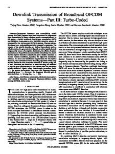
Fig. 1. The frame layer and the AV_GOP signal for the Terminator over a time window of 500 frames.

networking requirements, but is selected according to the video quality [32]. B. Basic Characteristics as

th GOP period will be denoted The average packet size at in the rest of this paper, and is given by

(1) denotes the integer part, the size of the MPEG-1 where the packet size at stream, and th frame. That is, for and the represents the frame size of frame at th GOP, , the first and frame of the same GOP, and so on. The dotted line in Fig. 1 illustrates the size of the first 500 frames of an MPEG-1 video sequence (Terminator Film). The , which is formed by exsolid line shows the signal so that it has the same size as the tending signal signal (perhaps apart from some last values when is not . integer). Particularly, it is held that and are also called the AV_GOP The signals and frame layer signal, respectively. In this figure, the large frame sizes correspond to frames, while the small ones correspond to frames, and the intermediate ones to frames. It follows video-sequence activity, is also observed that meaning that its size increases whenever the sizes of Intra and Interframes on average increase. This property is the basic concept behind the models relied on in the intermediate layer. Although frames have, on average, the largest size and the smallest one, models which ignore (or sometimes ) frames and take into account only frames severely underestimate the network resources [29]. This is due to the fact that and frames present higher fluctuation than frames, and that there is a strong correlation between them. The first reason stems from the coding algorithm of and frames. As we have stated above, some MB’s of and frames can be coded as Intra MB’s, resulting in low compression ratios. Consequently, during high video activity, the majority of frames within a GOP period, which mainly consist of Inter frames, take values which

96


TABLE I CORRELATION COEFFICIENT OF INTRA/INTER FRAMES FOR SEVERAL MPEG-1 SEQUENCES

are much greater than their average, therefore loading the network, while in low video activity, the values of frames within a GOP are small enough to empty the network buffers [35]. The strong correlation between Intra and Inter frames are due to the motion-estimation algorithm and the temporal continuity of the actual video stream. A correlation measure between two and , is given by the correlation stochastic processes, defined as coefficient (2) is the variance of a stochastic process, is where , the average of and the expectation operator, and , respectively. Table I shows the correlation coefficient between Intra and Inter frames for several MPEG-1 coded video sequences. In particular, our results have been obtained using four long-duration (40 000 frames) MPEG-1 streams: Terminator, Star Wars part III, and two TV series. The last three sequences are also called Sources 1, 2, and 3 in the following, for simplicity purposes. All the aforementioned sequences have been encoded using the same VBR coding control and encoding algorithm, such as the same quantization factors, motion-estimation method, and and GOP parameters. In this table, we show correlation coefficient values among Intra and Inter frames after being averaged over a GOP period. This is due to the fact that the correlation , and streams is not fair, since the reamong the entire spective elements of the streams correspond to totally different GOP’s. As it is observed, the correlation coefficient between Inter frames ( - ) is stronger than the respective one between Inter and Intra frames ( - , - ) since the coding method used for frames is different from the coding method used for Inter frames. Almost the same correlation degree is also observed for all the examined video sequences. Similar results as far as the , and frames is concerned, have also correlation between been presented in [29]. III. MODELING OF VBR MPEG-1 CODED VIDEO SOURCES The MPEG-1 stream corresponds to a low layer for modeling of VBR MPEG-1 coded video sources, in the sense that it contains all the statistical properties of the aggregate signal. In the following, we call this layer the frame layer, and call the respective signal the frame-layer signal. At this layer, we are able to generate models which can accurately approximate the network resources, since all the necessary information of the MPEG-1 signal can be exploited. However, the complexity of this signal, as it is briefly described in Section II, results in complicated traffic models requiring a large number of parameters.

Reduction of model complexity could be achieved by examining the MPEG-1 stream at a higher layer characterized by the following property: the signal on this layer should have a simpler form than the frame layer signal, but simultaneously provides an approximation of the aggregate sequence. Such a signal is , which appears the same average as the aggregate MPEG-1 sequence, follows video activity, presents smaller fluctuation than Intra and Inter frames, and is generally much simpler than the frame-layer signal. Modeling based on will be called GOP-layer the statistical properties of modeling in the rest of this paper. However, such modeling, without exploiting any other knowledge from the frame-layer signal, cannot provide sufficient approximation of the network resources due to the fact that significant characteristics of the aggregate MPEG-1 stream are lost, and the lost information is difficult to be estimated. For instance, for a given value , it is not possible to properly determine the size of , and frames within the respective GOP and their of erroneous estimation significantly affects the performance of the traffic models. The more knowledge about the MPEG-1 stream we exploit, the better approximation of the network resources we achieve, but simultaneously, the number of model parameters increases. At an intermediate layer, however, it is possible to efficiently and , generating combine the properties of models that can accurately approximate the traffic behavior of MPEG-1 sources requiring much smaller number of parameters. The basic concept of this layer modeling is to approximate video activity of MPEG-1 sequences using the simplified signal and according to the specific value of video activity (produced by the GOP layer model) to generate the sizes of , and frames using estimators based on frame-layer modeling. IV. FRAME–LAYER MODELING In the following, we study the statistical properties of the frame-layer signal i.e., the probability distribution and the autocorrelation function, and we propose traffic models capable of capturing the traffic characteristics of MPEG-1 video sources. A. Study of the PDF The frame size histogram of an MPEG-1 stream is characterized by many small values mainly due to and sometimes to frames and by few large values, mainly due to frames. The former causes a rapid increase at the region of frames of small size, while the latter a hill at the region of frames of large size. Consequently, the distribution of an MPEG-1 stream seems , to be superposition of three different distributions i.e., of and frames, meaning that it is more convenient to split the


Fig. 2.

Q–Q plots of Gamma and Lognormal Distribution for the Terminator. (a) Aggregate MPEG-1 stream. (b)–(d) I ;

MPEG-1 sequence into , and streams and perform separate statistical analysis for each of them. Fig. 2 illustrates the Q-Q plots (fractile diagrams [36]) of Gamma and Lognormal distribution of the Terminator for the frames. In aggregate MPEG-1 sequence, as well as for this figure, the quantiles are normalized by the respective maximum value of the real data. It is observed that, in contrast to , and frame histhe aggregate MPEG-1 sequence, the tograms can be approximated by Gamma or Lognormal distribution whose the unknown parameters are estimated using the method of moments [14]. Heyman et al. have also concluded that VBR teleconferencing streams follow the Gamma distribution using, however, another coding scheme [22].

97

P

, and B frames, respectively.

the negative peaks to frames, while the small positive peaks to frames. The periodicity of such a function is equal to the in our case), while the subperiodicity to the distance ( ( ). distance For this reason, separate study of the autocorrelation function for each type of frames is more convenient, since such an approach eliminates the periodicity of the aggregate sequence. , Fig. 3(b)–(d) presents the autocorrelation functions for and frames in case of the Terminator. The autocorrelation of frames decays more rapidly than of and frames, while the autocorrelation of frames presents the slowest decay rate. is said to have A stochastic process short-/long-range dependence if the sum of the autocorrelation at different lags converges or diverges, respectively [37], [38]. That is

B. Study of Autocorrelation Function In this subsection, survey of the autocorrelation function is performed. However, before presenting the basic properties, we first give some definitions for clarification purposes. at lag is The autocorrelation of a stochastic process defined as [2] (3) is the variance of the average, and where the expectation operator. Comparing (2) and (3), it seems . that parameters, the autocorrelation function Depending on of any VBR MPEG-1 coded video sequence appears “periodicity” and “subperiodicity” [35], as illustrated in Fig. 3(a) for and have been chosen as the Terminator, where GOP parameters. The large positive peaks are due to frames,

(4) for short-range dependent process (for long-range dependent process). Another equivalent condition for being a stochastic process short/long-range dependent is the asymptotic behavior of the variance of process with respect [39]. In particular, if the variance is proporto , for large , the process is characterized tional to decays at a as a short-range dependent, while if the , i.e., is proportional to , slower rate than for large , then the process is said to be long-range dependent. Estimating the parameter of several VBR MPEG-1 , and streams are coded video sources, it seems that long-range dependent processes [35]. Similar results can be

98


Fig. 3. Autocorrelation of the Terminator along with two AR models fitted to them. (a) Aggregate MPEG-1 stream. (b)–(d) I ;

found in [38], [40] for broadcast video sequences that have been coded using a hybrid DPCM/DCT compression algorithm. However, the performance of models that accomplish general statistical properties are not compulsory in agreement with that provided by real data. In [29], it has been shown that modeling relying only on statistical tests is not sufficient to approximate the network traffic, and consequently, deviation of some statistical properties is sometimes not so crucial as far as the network resources are concerned. Using Lindley’s equation for the delay in a G/G/1 queue, it can be shown that the long-range dependence property affects the network resources only if large busy periods occur. The term “busy period” indicates the time interval, starting when the buffer is empty and ending in the following empty state [40]. For a given utilization, we can assume that busy periods do not exceed a certain limit, and thus, lags beyond a threshold do not have any influence on the video traffic. As a result, there is a finite order of an AR model that can capture well the actual traffic, resulting in good prediction , and of frame/cell-loss probability. That is, the size of frames is estimated by (5a) with

and the AR order for the

-stream

(5b)

is the th frame size for the -stream generating where , and is the independent by the AR model of order

P

, and B frames, respectively.

and identical distributed noise with zero mean and variance one. The model parameters , , and are estimated using the Yule–Walker equations [41]. Based on the Yule–Walker equations, the AR model parame, and ters are obtained by examining the entire sequences of frames. This approach is useful for estimating the network resources during the network design phase, using, e.g., the traffic models as video generators. However, in applications where dynamic bandwidth allocation or prediction of frame sizes or activity during video transmission is necessary, an adaptive implementation of the Yule–Walker equations is performed, modifying the AR parameters in every, e.g., GOP period [41]. Both approaches are discussed in the section of experimental results of this paper. Fig. 3(b)–(d) illustrates the autocorrelation functions of an AR model of order 1 [AR(1)] and a high order AR for the Terminator sequence, whose the unknown parameters have been calculated based on statistical properties of the entire sequence of Intra and Inter frames. It is observed that AR models of high order better approximate the autocorrelation than AR’s of , , and order 1. In particular, an order of has been used for each type of frame of the Terminator sequence. In general, the following inequalities are satisfied. Fig. 4 illustrates the autocorrelation functions of video Sources 1, 2, and 3 along with the respective of the Terminator , and frames. All the examined sequences present for similar behavior as far as the autocorrelation function is concerned. In particular, Sources 1 and 2 present slightly slower


99

Fig. 4. Autocorrelation of the Terminator compared with various MPEG-1 sources. (a) I frames. (b) P frames. (c) B frames. TABLE II CORRELATION COEFFICIENT OF THE PREDICTION ERRORS OF INTRA/INTER FRAMES FOR SEVERAL MPEG-1 SEQUENCES

decay than the autocorrelation function of the Terminator. On the contrary, a slightly faster decay appears in the autocorrelation of Source 3. As a result, the high-order AR models, used for capturing the statistical properties of the Terminator, are also appropriate for the other three streams. This is due to the fact that the Terminator is a long duration sequence, containing all possible variations of the video activity, such as camera zooming and panning, abrupt scene changes, and periods with high/slow motion. Therefore, examining the statistical properties of the Terminator is adequate to provide satisfactory results for the other video sequences, too. In case, however, of sources with specific characteristics, better performance of the proposed models is achieved through categorization of video sequences into classes. In such cases, the modeling procedure remains the same, while the model parameters are estimated using some representatives of the class. C. Traffic Model of Frame Layer (Model A) Based on the statistical properties presented in the previous with subsections, three high-order AR models, , can be used for modeling of , and streams. Then, the generated signals are deterministically merged, acparameters of the GOP pattern, to form the cording to and estimated frame layer signal. However, if uncorrelated predicare used as filter inputs to generate the signals tion errors , the aggregate MPEG-1 sequence will contain uncorre, and components, instead of real data, where , lated and frames are strongly correlated, as we have discussed in Section II. In this case, the estimated aggregate sequence does not present the burstness of the real data, resulting in poor estimation of the network resources. , Indeed, the statistical properties of prediction errors obtained using the inverse AR filter (where real data are used as the filter input, while the filter output corresponds to the respec-

tive prediction error), indicate that there is correlation among them. Table II shows the correlation coefficient of predictions errors of , and frames after being averaged over a GOP period, for the four examined MPEG-1 video sources. This is done for the same reason as in Section II. As it is observed, the correlation coefficient between prediction errors of Inter frames is higher than the respective coefficients of Inter and , and Intra frames. Correlation among prediction errors of frames stems from the correlation among , and frames themselves, as we have mentioned in Section II. follow Another interesting property is that the errors the same p.d.f. as illustrated in Fig. 5, where the quantiles of prediction errors corresponding to and frames are depicted versus the quantiles of errors of frames for the Terminator and Source 1 video sequence. The previous property results from , and frames the fact that the frame size histograms of conform to the same p.d.f. as we have stated in Section IV-A. , and prediction errors is reAs a result, correlation of quired to generate a model for the aggregate MPEG-1 sequence, , and components. Howwhich will contain correlated ever, using the second property, an approach to correlate the eris to generate a reference error signal, which follows rors , and then, generate the prediction errors the same p.d.f. as based on this reference signal. A simple method is to consider the error of frames as reference error, due to the fact that frames constitute the majority within a GOP. Then, the errors of and frames are related to that of frames through a correlation mechanism illustrated in Fig. 6, which is also called Model A in the following. In particular, to generate the prediction error of frames, , the error of frames, is related to using the following equation: for odd otherwise

(6)

100


Fig. 5. Q-Q plots of I and P prediction errors with respect to the error of B frames. (a) Terminator sequence. (b) Video Source 1 sequence.

Fig. 6.

Block diagram of the proposed model at the frame layer (Model A).

where is the number of frames within a GOP and is the the prediction error corresponding to the second frame within the GOP period. In general, as , we denote the of a GOP. In Fig. 6, (6) is prediction error of the th frame depicted through the decimator filter ↓, whose the input–output , after relationship is given by shifting the reference error by one lag. frames are fed with the Equation (6) indicates that and same prediction errors for every odd group of the picture period. The correlation coefficient of the errors of and frames after being averaged over a GOP, achieved by this mechanism, is close to that provided by the real data (Table II). In particular, and provided by the the correlation coefficient of model over a GOP period is equal to 0.17. It should be men, and frames tioned that since by definition the errors of present zero mean and variance of one, there is no need for the to be shifted or be scaled to compensate reference error probable differences in mean and variance. Instead the parameters involved in (5a) are used to shift and scale the respective prediction errors so that the generated signals present the appropriate mean and variance.

Similar procedure is used for generation of error. In into three error sequences, denoted particular, we split , , each of which corresponds to the error by of the th frame, say , within a GOP. This means that indicates the error of the first frame within a GOP, while refers to the second frame, , and to the third is split into sequences where one, . In general, the denotes the number of frames within a GOP. Then, each is related to the reference error as follows: error (7) in our case. The previous with , and frames of a GOP are equation means that the , and generated using the same prediction error as the frames. , we can easily Having estimated the errors by merging them into a common link as produce the error it illustrated in Fig. 6 using a mixing “switch”. Such an approach results in correlation coefficient between the errors of and frames over a GOP period equal to 0.61, which is close to that presented in Table II for the real data. Correlation between the errors of and frames is indirectly achieved through (6), (7).


101

Fig. 7. Q-Q plots of Gamma and Lognormal distribution for the GOP layer signal for the Terminator. Fig. 8. Autocorrelation of the GOP layer signal and of two AR models fitted to it for the Terminator.

In cases that a different degree of correlation is necessary among the prediction errors, a different proportion of correlation should be performed. For instance, weaker correlation is accomplished to be uncorrelated to the reference by leaving the error . error V. GOP LAYER MODELING In this section, we propose video source models at the GOP . layer by examining the statistical properties of signal A. Statistical Analysis The quantiles [36] of Gamma and Lognormal distribution are presented in Fig. 7 for the versus the quantiles of Terminator sequence. In this figure, we depict the quantiles normalized with the respective maximum value of the real data, as we have done in Section IV-A. We observe that both Gamma and Lognormal distribution fits well the real data for both video sequences. Studies of others MPEG coded video sources have resulted in similar conclusions as far as the histogram of is concerned [35]. is depicted in The autocorrelation function of Fig. 8 (solid line). Using similar ideas to those discussed in Section IV-B, we can approximate the autocorrelation of with a high order AR model. In general, the order of the AR is close to the order of the respective AR of frames since a similar decay rate is presented. In Fig. 8, the dashed and dotted lines correspond to the autocorrelation functions of an AR(1) and an AR(20) model, respectively. Fig. 9 illustrates the for video Sources 1, 2, and autocorrelation functions of 3 along with that resulted from the Terminator. In particular, the autocorrelation functions of Sources 1 and 2 decay slightly slower than that of the Terminator while the autocorrelation of Source 3 presents a slightly faster decay. However, in all cases, the differences of autocorrelation are very small and thus, modeling based on the Terminator is adequate to capture the statistical properties of the other three streams. B. Traffic Models of GOP Layer , a highHaving examined the statistical properties of order AR can be used for its modeling. However, in this layer,

Fig. 9. Comparison of the autocorrelation of the GOP layer signal of the Terminator with various MPEG-1 sources.

regardless of the sequences used for modeling and evaluation, refers to an average the proposed traffic model, say, signal over a GOP period, instead of the aggregate MPEG-1 sequence, which actually determines the network resources. Thus, the problem is how to estimate the frame sizes within a GOP, . Coarse estimation of the for a given value of signal frame sizes results in poor traffic approximation, meaning that the proposed models overestimate or underestimate the actual traffic, whereas good performance is achieved by accurate prediction of frame sizes. The degree of estimation depends on the proportion of knowledge, which we exploit from the frame layer signal and the method we use for the frame size prediction. In the following, we analyze the case of no or small knowledge about the frame layer signal as Methods A and B, respectively, while in Section VI we efficiently combined properties of sigand to generate models that are good estinals mators of frame/cell-loss probability requiring a small number of parameters. Method A: In this case, we assume no knowledge about the properties of frame layer signal. Therefore, we can estimate the frame sizes of MPEG-1 sources by considering all frames within . Fig. 10 a GOP to be equal to the respective value of

102


Fig. 10.

Graphical representation of Method A of GOP layer.

Fig. 11.

Graphical representation of Method B of GOP layer.

presents the proposed scheme, where denotes the estimation of the aggregate MPEG-1 sequence using Method A. As is the same as , which has been we can see, does not fulfill the stadefined in Section II. The signal tistical properties of MPEG-1 sequences since neither the distribution function nor the autocorrelation function is satisfied. Only are fulfilled. The above-dethe statistical properties of scribed simple approach can be used only for an initial estimation of the network resources. The adopted method underestimates the average size of frames, while it overestimates the size of and frames. However, at no multiplexing schemes and at conventional utilization, i.e., around 0.8, the small size of frames is balanced with the large size of and frames resulting in good estimation of frame/cell-loss probability. On the other hand, at multiplexing schemes where the entire stream is tend to smooth out around its average, the large frames and the high fluctuation of and frames, which is underestimated by this methodology, mainly determine the network resources. Therefore an approximate estimation of the traffic behavior is achieved. Method B: In this case, we assume that small knowledge about the properties of frame-layer signal is available. In partic, and frames, ular, we consider that the mean values of respectively, are given. Then, the estidenoted by mated frame size of Intra and Inter frames is given by (8) and are the mean value of signal . Equation (8) indicates that the estimated frame size of Intra/Inter frames is proportional to the ratio of mean value of the respective type of frame and the average value of signal . The proposed method is presented in Fig. 11, where indicates the generated signal using Method B. It is expected that this method gives better estimation as far as the network resources are concerned, in relation to Method A. However, it does not still capture the high fluctuation of and frames and the large values of frames, resulting in

where

poor estimation of frame/cell-loss probability, especially at multiplexing schemes. VI. INTERMEDIATE LAYER MODELING As we have stated above, Methods A and B provide approximate estimation of frame/cell-loss probability. Further improvement of the network performance is achieved if more information about MPEG-1 stream is exploited. As knowledge increases, the required number of parameters increases too. This means that we are moving from the high GOP layer to the low frame layer, and when all knowledge about the frame-layer signal is available, modeling results in frame-layer modeling. However, there is an intermediate layer, where we are able to reduce the number of parameters while satisfactorily approximating the network resources, since significant parts of information of both layers can be combined. The basic concept is: 1) to simplify the GOP layer models so that only video activity is estimated and 2) to introduce simplified models for Intra and Inter frames, based on the estimated video activity. In a VBR coding mode, in case of high video activity, the encoder rate is much larger than the average, since more bytes per frame are allocated to maintain the requested picture quality. On the contrary, in low video activity, the rate drops. Since the output rate of the statistical multiplexer is constant, high video activity fills up the buffer, causing frame/cell-loss probability, while low video activity empties the buffer. When the encoder rate is around the average-medium activity, the state of the buffer remains almost constant, presenting small fluctuations. Thus, categorization of the size of Intra/Inter frames into different video activities (bands) is useful for modeling, since each band affects the network resources in a different way. Fig. 12 illustrates the general structure of the proposed model at the intermediate layer. It consists of three subsystems: the activity model subsystem, band selection subsystem, and band , and frames. model subsystem for 1) Activity-Model Subsystem: The purpose of this subsystem is to approximate the video activity and the burstness


103

Fig. 13. Autocorrelation of parameter .

Fig. 12. Block diagram of the subsystems that form the intermediate layer model (Model B).

of MPEG-1 coded video sources based on properties of signal . This means that the activity is estimated on a GOP basis. Its output activates the band selection subsystem. 2) Band-Selection Subsystem: This subsystem is the link between the activity-model subsystem and the band-model subsystem. It takes as input the output of the activity-model subsystem and, according to its value, selects the appropriate band and the respective parameters for the band model. 3) Band-Model Subsystem: It is the subsystem responsible , and frames within a GOP. Taking at for generation of the beginning of each GOP the proper parameters and the selective band provided by the band-selection subsystem, it comdistances. poses the MPEG-1 stream according to and In the following, we perform statistical analysis for each band which is required to find the structure of the band models and to estimate their unknown parameters. A. Band Statistical Analysis is used to classify the video sequences The signal into activity bands. In particular, groups of picture whose the is greater than a predetermined respective value of , are marked as high-activity GOP’s. Instead, threshold, say, below a threshold, say, , GOP’s with values of are considered to correspond to low activity band. Values of between the threshold and defines GOP’s of medium activity band. As a result, video activity is selected on a GOP basis.

B

frames in high band for various values of

All , and frames, whose the respective groups of pic, and high ture belong to a high activity band, are called , and medium band frames. Similarly, we can define the (low) band frames. Based on the results obtained by the statistical properties and characteristics of each band frame, proper , and frames within each traffic models for generating band are proposed. First, we consider the temporal behavior of band frames by examining their autocorrelation function for difand . Fig. 13 illustrates the auferent values of thresholds tocorrelation function of frames in high band using different , in the case of the Terminator. In this values of threshold is given in relation to the mean and the figure, the threshold , that is standard deviation of the signal (9) is the parameter which denotes how far the threshold where is from the average, and is the standard deviation of . Similarly, we can determine the low threshold by subtracting the average from the standard deviation multiplied by the scaling factor . As is observed by comparing Fig. 4(c) and Fig. 13, the autocorrelation functions of frames in the high band decay more rapidly than the respective of the aggregate frames. Similar results are found for and frames. Hence, it is anticipated that AR models of much lower order can be used to approximate the frame size in high band. , or equivalently, parameter , In particular, threshold is selected in such a way that an AR(1) sufficiently models the temporal behavior of high band frames. This is accomplished by minimizing a cost function expressing the average distortion between the autocorrelation function of each band frame, resulting , and the respective AR(1) model from a given value of

(10) where , or the

is the vector containing the autocorrelation of frames in the high band at the first lags, and

104


Fig. 14.

(a) Average distortion versus

for high band. (b) Distortion of I;

Fig. 15.

Autocorrelation for high band of Terminator and various MPEG-1 sources.

is the respective vector for the AR(1) model. In our . simulation, Fig. 14(a) presents the cost function of (10), after applying a low-pass filter to eliminate noisy fluctuations. Fig. 14(b) for each type of frame. shows the respective cost function that minimizes the average cost distortion The value of is very close to that which minimizes the distortion for each type of frames in the band. Thus, the resulting threshold is appropriate to model all band frames as an AR of order 1. The thresholds obtained by examining the other three sequences are close to that obtained by the Terminator. However, a small fluctuation of the threshold around the value obtained by this method is not so significant for the traffic behavior since the autocorrelation is slightly affected. The autocorrelation functions of video Sources 1, 2, and 3 along with the respective autocorrelation of the Terminator sequence are presented in Fig. 15 using the previously obtained . Good approximation is observed in value of threshold almost all cases. Similar results can be verified for low and medium band. B. Traffic Model of Intermediate Layer (Model B) After performing the band statistical analysis, we concentrate on the implementation of the proposed scheme using the block diagram of Fig. 13.

P , and B frames versus

for high band.

1) Activity-Model Subsystem Implementation: The implementation of this subsystem is based on signal (GOP layer), and its goal is to approximate the video activity. The is split into three activity bands. Large values of signal correspond to a high activity band, medium sizes to a medium activity band, and finally, small sizes to a low activity band. Since the probabilities of staying in an activity band almost drop exponentially, the video activity can be modeled as a three-state Markovian chain whose the states correspond to high, medium, and low activity bands. of the Markovian chain will The transition matrix be estimated as follows ([22]): number of transition to number of transitions out of

(11)

when the denominator is greater than zero. Since the sum of elements of the transition matrix for every row is equal to one, six parameters are required for video activity modeling. 2) Band-Selection Subsystem Implementation: A simple retrieval mechanism is used for finding the appropriate parameters of the band models subsystem according to the value of video activity. 3) Band-Model Subsystem Implementation: Based on the , and streams within each autocorrelation functions of band, three AR models of order 1, each of which refers to the , and frames, are used for modeling of each band. Since


105

Fig. 17. Buffer configuration scheme.

Fig. 16.

Proposed Model B.

frames of the medium band preserve the current buffer status while frames of the low band empty the buffer, the exact values of frames in low and medium band do not play a significant role to the traffic behavior, but only their respective average. As a result, we can consider the frame size within the low and medium band constant and equal to the average. Although this approach does not satisfy the statistical properties of the medium and low band, it approximates very well the traffic intensity of video sources, and simultaneously reduces the required number of parameters to six, two for the bands and , and frames. On the contrary, three AR three for the models of order 1 are used for modeling the size of frames in high bands, since a high band significantly affects the loss rates. Thus, the required number of parameters used for modeling frames in high bands is equal to nine, i.e., three for each AR model and three for each type of frames, resulting in a total number of 21 parameters: six for the Markovian chain, nine for the high band, and six for the other bands of the model, meaning that seven parameters for each frame type are on average required. 4) Model-B Description: Fig. 16 presents the model at the intermediate layer (Model B) relied on the previous subsystem implementation. The three-state Markovian chain corresponds to the video activity model whose the states indicate the high (HB), medium (MB), and low (LB) activity band. At the beginning of every GOP, a video activity is selected according to the transition probabilities of the Markovian chain. The Markovian chains inside the states of the video-activity model (the “small” chains) describe the structure of the GOP, as it is defined by the and distances. For instance, having generated the frame for a GOP, which is the first frame, the chain transits with probaframe (first frame in the GOP), and then with bility one to frame (second frame in the GOP) and probability one to so on. Each state of the “small” Markovian chains corresponds to the output of the respective band model. That is, LIo is the output of the Low Band model for the frame, i.e., a constant value, while HPo is the output of high band model for the frame, i.e., an AR(1). VII. BUFFER CONFIGURATION SCHEME To evaluate the good performance of the proposed traffic models as far as the network resources are concerned we have

used the following buffer configuration scheme illustrated in Fig. 17. independent video sources are multiplexed into a common buffer connected to a single ATM link. A first-in first-out (FIFO) policy is considered for the statistical multiplexing, meaning that cells are stored, and leave the buffer in the same order as they enter it. A cell can get into the common buffer only if there is available space for it. Otherwise, it is lost along with the respective frame. The output rate of the buffer is assumed to be mean , where is number of constant and equal to the multiplexed sources, the utilization, and the average source rate. For every frame period, the frame size is calculated using either the real data or the aforementioned source models. The real data have been obtained by recording several VBR MPEG-1 coded video sequences of long duration using the encoding algorithm described in Section II. In case of source models, several sets of traffic data (paths) are created and the results are obtained by running many times the simulation for each different sample path. In particular, eight different paths have been selected in our experiments. To generate traffic for different sources, we have used the same data sequence but different initial frames, as in [22]. The starting times of the multiplexed video sources significantly affect the cell-loss rates even though the sources present identical statistical characteristics. Since every frame of each video sequence arrives at a constant time, equal to the frame period, a video source that starts its transmission a short time after the other sources will have many more losses. As a result, frames arriving from this source are more likely to face larger queue lengths than cells arriving earlier from other sources, in the sense that the arrival-instant queue seen by different sources is not statistically identical. An approach, to reduce, this so called source-periodicity effect, which has been observed in [22] for video traffic, is to uniformly distribute the starting times of the multiplexed sources in intervals of 40 ms. This assumption sources appear at the multiplexer at is valid in case that the random time instances. However, in applications when many video sources are synchronized to start their transmission at the same time, the uniform distribution of the starting times within an interframe interval is not satisfied [22]. Although in such a scenario, the average loss rate will be greater than the respective rate obtained using a uniform distribution of starting times, the most important issue is that the traffic behavior of some sources will be quite different from some other ones. In this case, if the traffic behavior is examined based on the source of the worst losses, the network resources will be insufficiently allocated. As a result, reduction of the source periodicity effect is necessary for efficient transmission of video sources.

106


Fig. 18. Frame/cell-loss probability versus buffer size using data of various MPEG-1 sources and Model A at different utilization in case of uniform p.d.f. for the starting times. (a), (b): U = 0:75. (c), (d): U = 0:85:.

Two methods are presented in this paper for reduction of the source-periodicity effect. The first one is based on a non-FIFO scheduling policy at the multiplexer, while the second on a histogram equalization, which transforms the distribution of starting times to a uniform one. In the FIFO buffer policy described above, when a new cell arrives at the buffer and finds it full, it is automatically dropped, regardless of the current losses of the respective source. On the contrary, in the non-FIFO scheduling policy, an accumulated loss rate for each source is calculated. Then, an arriving cell that finds the buffer full, it is not automatically dropped. Instead, the cell, corresponding to the source with the lowest current accumulated losses among all cells being in the buffer, is dropped, resulting in an equalization of the loss rates over all sources. This scenario does not affect the average cell rate, which remains the same as in the FIFO case, since it decreases the cell rate of some sources at the expense of some others [22]. In the second approach, a histogram equalization of the starting time distribution is performed. Let us denote the cumulative distribution of starting times within an interframe ms. Experiments can define the interval, by . Let be the cumulative function shape and type of of the uniform distribution. Hence, any time stamp, say, in

the time interval of 40 ms, corresponding, for example, to the starting time of the th source, is mapped to a new time (12) so that the distribution of the new starting times follows the uniform p.d.f. Equation (12) indicates that an additional delay should be added to the th source. However, in the of , this additional delay is negative, meaning case where that the th source should start its transmission earlier. Since this is practically impossible, the starting time of the respective source is determined within the following interframe period, i.e., ms. Such an approach, although reducing the average losses of the multiplexed sources, increases the source delay, 40 ms at maximum. VIII. EXPERIMENTAL RESULTS The proposed traffic models are evaluated using three VBR MPEG-1 coded video sequences, different from that used in modeling. A. Frame-Layer Model (Model A) First, a uniform distribution of the starting times and a FIFO scheduling policy is considered. Fig. 18 presents frame/cell-loss


107

complished, this is balanced by the additional delay introduced by this methodology, as we have mentioned in Section VII. This additional delay is also presented in Table III for each of the 20 multiplexed sources. Since, on average, an additional delay of about 20 ms is introduced, we conclude that the average losses at the same total delay (buffering plus histogram equalization delay) is slightly better to that provided by the non-FIFO scheduling policy (see Table III). As a result, synchronized video sources require greater delay to achieve the same video quality. However, in the non-FIFO scheduling policy, smaller loss fluctuation is observed. Since this method is independent form the p.d.f. of starting times it can also be applied in the uniform distribution for further equalizing the source losses. Fig. 19. Comparison of cell losses in case of synchronized and uniformly distributed sources and the performance of Model A and B for the former case.

probability versus buffer size of a signal generated using the proposed Model A and real data recorded from the video Sources 1, 2, and 3 at a wide range of utilization (0.75 and 0.85), in the . The simulation was performed with the data case of rate scaled up and down by 2% to show how close the estimated loss probability is to that obtained from the real data [15], [26]. Although a slight deviation out of the range of 2% is observed, , Model A seems to be robust for estiespecially at mating frame/cell losses. In case of many synchronized video sources, different buffer statistics are expected to be encountered since many frames arrive at the same time with high probability. In our simulations, a Gauss distribution has been used for modeling the starting times instead of the uniform one used in the previous case. Fig. 19 presents a comparison of the average cell losses versus buffer size for video Source 1, using as starting-time p.d.f. the uniform and the Gauss distribution. In this figure, 20 sources have been multiplexed. The uniform p.d.f. is defined in the interval of [0 40] ms, while the Gauss by an average of 20 ms and standard deviation of 0.1. The latter means that the majority of sources start their transmission at the middle of the interframe interval (around 20 ms). Although the same utilization has been used, higher cell losses are observed in case of synchronized sources, for all buffer sizes. In this figure, we also illustrate the estimated cell losses, provided by Model A. Good approximation is noticed in all buffer sizes since the proposed model is based on the statistical properties of video sources. Table III presents the cell losses for each of the 20 individual multiplexed sources for two delay values (105 ms and 82 ms) and utilization equal to 0.85 when the aforementioned Gauss p.d.f. has been used as distribution of the starting times. Although the multiplexed sources present the same statistical properties, they are characterized by very different loss rates. In particular, many sources present no losses at all, even for small buffer sizes, whereas there are sources, such as source 4 and 15, where the respective losses are much higher than the rest ones. In the same table, the results obtained by applying the non-FIFO scheduling policy and the histogram equalization, as they have been described in Section VII, are also presented. In both approaches, reduction of the source-periodicity effect is noticed. Although in the second approach, an improvement of the average cell-loss rate is also ac-

B. GOP Layer Models (Methods A, B) Fig. 20 presents the cell-loss probability using the Methods A and B of GOP layer modeling for the Terminator. Our simulations were done with 20 multiplexed video sources and using the uniform distribution for the starting times. Even though the Terminator sequence has been used for evaluation, both methods underestimate the loss probability. This is due to the fact that at multiplexing schemes, where the aggregate video stream tends to smooth out around its average, the burstness of MPEG-1 video traffic, which cannot be estimated by Methods A and B, affects the cell losses. However, it seems that Method B better approximates the loss probability since more information of the frame layer signal is exploited. For this reason, GOP layer modeling can be used only for an initial estimation of the video traffic characteristics, i.e., for capturing the activity of a video source. C. Intermediate Layer Model (Model B) The accuracy of the proposed traffic Model B, as far as the frame/cell-loss probability is concerned, is evaluated in Fig. 21, . Our simin the case of video Sources 1, 2, and 3, when ulation has been performed using the uniform distribution for the starting times, while the parameters of Model B have been estimated based on the Terminator sequence. Despite the significant reduction of the required model parameters, a very good approximation of frame/cell losses is observed in a wide range of utilization (0.75 and 0.85). As in frame-layer modeling, the data losses are obtained by varying the data rate 2%. A slight deviation out of the range 2% is also observed for some buffer sizes, especially at low utilization, meaning that Model B is very robust for estimating the MPEG-1 traffic behavior. The performance of the proposed Model B for each individual source is presented in Table III using the same conditions as those described in the frame-layer modeling. It seems that Model B approximates well both the average and the individual loss rates. The performance of the proposed Model B in case of synchronized video sources is presented in Fig. 19. As it is observed, Model B provides a very good approximation of the cell losses for all buffer sizes since, as with Model A, Model B does not depend on the adopted starting time distribution of the multiplexed sources. D. The Effect of Delay In the following, the effect of a large buffer size to the system delay is examined. In general, a number of components

108


TABLE III AVERAGE CELL LOSS PROBABILITIES FOR DIFFERENT DELAY AND BUFFER CONFIGURATION SCHEMES AT UTILIZATION 0.85

Fig. 20. Cell-loss probability versus buffer size using data of the Terminator and Method A and B of GOP layer at U = 0:8.

introduces delays in a video transmission system: encoder buffering, frame reordering necessary for decoding of frames, actual encoding and decoding time, network transport delays and so on. In case of highly interactive videoconference applications or real time video transmission, low delays are usually preferable. Furthermore, the overall delay may be one of the negotiated QoS parameter that the network should guarantee [18]. In this paper, we concentrate on buffering delay, which is required to smooth VBR traffic into CBR one. This delay is of particular interest since it influences both video quality and the multiplexer gain through the associated traffic characteristics [32]. For constant frame-rate encoders, like the examined MPEG-1, the overall delay throughout the system should be constant for the duration of the connection. This is due to the fact that once decoding starts, a video frame should be displayed every 40 ms.

As a result, the time between the capturing and the displaying of a frame should remain constant. Since the number of bits per frame is variable due to the VBR coding, the end-to-end delay should guarantee that the decoder can access all bits of a frame by the time that the frame is required to be displayed. As a result, the buffering delay is measured as the maximum delay required by a cell to get out of the buffer [22], [32]. Fig. 22 presents the delay versus the number of multiplexed video sources for the Terminator sequence in case of 0.85, 0.8, and 0.75 utilization. In particular, in this figure, the delay is obtained by using such buffer size that a 10−5 average cell-loss rate is accomplished. As it is observed in Fig. 22, for utilization above 0.8, the delay, even for many multiplexed video sources, is greater than the frame reordering delay for frames, which in our case is equal to 80 ms (two successive frames). In particular, in the and , the buffering delay is 139 ms case of for 10−5 average cell loss. This is also presented in Fig. 23, which illustrates the delay versus utilization for 20, 15, and 10 multiplexed sources for the same loss probability. Furthermore, our simulations indicate that the delay is high for small number of multiplexed sources, even in case of low utilization. Specifically, and , a delay of 371 ms is measured, when which is 4.64 times greater than that of 80 ms. As the number of multiplexed sources increases, the delay decreases too, even for and , a delay the same utilization. Indeed, for comparable to the interframe period is noticed. E. Prediction of Video Activity In applications where we are interested in prediction of video activity, an adaptive implementation of the proposed AR models is accomplished. Such applications are very useful for dynamic bandwidth allocation or effective implementation of congestion-control schemes, especially over ATM networks responsible for maintaining the negotiated QoS. In this case,


109

Fig. 21. Frame/cell-loss probability versus buffer size using data of various MPEG-1 sources and Model B at different utilization in case of uniform p.d.f. for the starting times. (a), (b) U = 0:75. (c), (d) U = 0:85.

Fig. 22. Delay versus the number of multiplexed sources in case of average loss probability equal to 10−5 for the Terminator.

Fig. 23. Delay versus utilization in case of average loss probability equal to 10−5 for the Terminator.

based on the previous samples of the transmitted sequence, the current video activity is predicted through an adaptive procedure described in the following. Such an approach increases the prediction accuracy and provides the system with the flexibility of satisfactorily estimating future samples.

An AR model is considered more suitable for such an adaptive implementation, due to the fact that the current estimated value is expressed as a function of the previous values and to the fact that its parameters have been estimated as it is presented in [41].

110


smoother tracking capabilities. We observe that the model predicts the actual traffic very accurately, despite the small time delay at the instances of band changes. The plot of the first AR coefficient versus GOP indices is illustrated in Fig. 25 along with the respective actual data for indicating the actual tracking capability of the model. After a video activity change, the AR coefficient takes a small value. In the following samples, the AR coefficient increases, since samples with more similar statistical properties are included to the observable data. After the band prediction, it is possible to estimate the values of Intra/Inter frames within a GOP using a similar adaptive framework.

IX. CONCLUSION

Fig. 24.

Prediction of video activity for 100 GOP indices.

Fig. 25.

The first AR coefficient versus GOP indices.

In particular, the adaptive implementation of the AR model is performed on a GOP basis and the current band is predicted samby exploiting the statistical properties of the previous ples. In order to impose different significance on each of the previous samples and to afford the possibility of following the statistical variations of the observable data, a forgetting factor is introduced. This means that samples, which are far from the current GOP index, affect the statistical properties less than samples close to it. In our simulation, ten samples have been used as observable data, while the forgetting factor is chosen to have , with for each th prethe following form: vious sample. Fig. 24 shows the tracking capability of the proposed model to the actual data in case of an AR model of order 2. In this figure, 100 GOP indices are illustrated, taken from the Terminator sequence. The zero value corresponds to low activity band, while values of one and two correspond to medium and high activity band, respectively. The use of an AR(2) instead of an AR(1) is based on the fact that the latter provides much

In this paper, we survey the traffic characteristics of multiplexed VBR MPEG-1 coded video sources transmitted over ATM B-ISDN networks. We also propose traffic models, which approximate the network resources: frame/cell-loss probability and buffering delay. Our study has concentrated on three layers: the frame layer, GOP layer, and Intermediate layer. In the first layer, the aggregate MPEG-1 stream, which constitutes the frame-layer signal, is examined, and a correlated AR model of high order (Model A) is introduced to approximate the network resources. Reduction of the required parameters is achieved by analyzing the MPEG-1 video sources at a higher is used layer (GOP layer) on which a simpler signal for modeling. However, without enough knowledge about the frame-layer signal, models on this layer are not good estimators for the MPEG-1 traffic characteristics. In order to maintain accurate approximation of the MPEG-1 traffic behavior and simultaneously reduce the number of required parameters, an intermediate layer, which efficiently combines properties of the other layers, has been introduced in this paper, resulting in Model B. Experimental results and simulation using several VBR MPEG-1 coded video sources have shown the ability of both Model A and B to successfully approximate the network resources at a wide range of utilization. However, since the parameters of Model B are much simpler than that of Model A, we can conclude that the most suitable layer for modeling MPEG-1 sequences is the Intermediate layer. Our simulations have concentrated on the impact of the buffering delay to the VBR MPEG-1 stream at a wide range of utilization and several multiplexed sources. In applications where dynamic bandwidth allocation or admission control is necessary, prediction of the video activity bands can be examined based on an adaptive implementation of the AR model. Our investigation indicates good tracking capabilities of the adaptive model to the actual data. Of particular interest is the relation of frame/cell-loss probability to the visual distortion, which is observed by the human eye. Although loss probability is a metric which indicates how well the models estimate the network resources, this value does not directly corresponds to the visual distortion of video signals. For instance, the loss of a frame is not generally as significant as the loss of an frame, since in the latter case, all frames within a GOP will be distorted.


ACKNOWLEDGMENT The authors would like to thank all the anonymous reviewers for their constructive comments and useful suggestions that helped in improving the quality, presentation, and organization of the paper. They would also like to thank Prof. Kollias for his fruitful remarks.

REFERENCES [1] L. Chiariglione, “MPEG and multimedia communications,” IEEE Trans. Circuits Syst. Video Technol., vol. 7, pp. 5–18, Feb. 1997. [2] N. Ohta, “Packet Video,” in Modeling Signal Processing. Boston, MA: Artech House, 1994. [3] M. de Prycker, Asynchronous Transfer Mode, Solution for Broadband ISDN. Antwerp, Belgium: Alcatel Bell, 1993. [4] ITU-T SG 15 Experts Group for Very Low Bitrate Visual Telephony, Draft Recommendation H.263, Feb. 1995. [5] ISO/IEC 13 818-2, Generic Coding of Moving Pictures and Associated Audio, H.262, Committee Draft, May 1994. [6] N. Doulamis, A. Doulamis, Y. Avrithis, and S. Kollias, “Video content representation using optimal extraction of frames and scenes,” in Proc. EEE Int. Conf. Image Processing (ICIP), Chicago, IL, Oct. 1998, pp. 875–877. [7] ISO/IEC JTC1/SC29/WG11 N1678, MPEG-7: Context and Objectives (v.3), April 1997. [8] S.-F. Chang, A. Eleftheriadis, and D. Anastassiou, “Development of coloumbia’s video on demand tested,” Signal Processing: Image Commun., vol. 8, pp. 191–208, 1994. [9] N. Doulamis, A. Doulamis, D. Kalogeras , and S. Kollias, “Low bit rate coding of image sequences using adaptive regions of interest,” IEEE Trans. Circuits Syst. Video Technol., vol. 8, pp. 928–934, Dec. 1998. [10] M. Tekalp, Digital Video Processing. Englewood Cliffs, NJ: PrenticeHall, 1995. [11] M. ISO/CD 11 172-2, Coding of Moving Pictures and Associates Audio for Digital Storage Media at up to about 1.5Mbps, Mar. 1991. [12] T. Sikora, Digital Electronics Consumer Handbook, MPEG Digital Video Coding Standards, R Jurgens, Ed. New York: McGraw Hill, 1997. [13] B. Maglaris, D. Anastassiou, P. Sen, G. Karlsson , and J. D. Robbins, “Performance models of statistical multiplexing in packet video communication,” IEEE Trans. Commun., vol. 36, pp. 834–843, 1988. [14] A. Papoulis, Probability Random Variables and Stochastic Processes. New York: McGraw-Hill, 1984. [15] M. R. Frater, J. F. Arnold, and P. Tan, “A new statistical model for traffic generated by VBR coders for television on the broadband ISDN,” IEEE Trans. Circuits Syst. Video Technol., vol. 4, pp. 521–526, 1994. [16] G. I. Stassinopoulos, I. S. Venieris, K. Petropoulos, and E. N. Protonotarios, “Performance evaluation of adaptation functions in ATM environment,” IEEE Trans. Commun., vol. 42, pp. 2335–2344, 1994. [17] G. I. Stassinopoulos and I. S. Venieris, “ATM adaptation layer protocols for signaling,” Comput. Networks and ISDN Syst., vol. 23, no. 4, pp. 287–304, 1992. [18] A. Adas, “Traffic models in broadband networks,” IEEE Commun. Mag., vol. 35, no. 7, pp. 82–89, 1997. [19] P. Pancha and M. El Zarki, “Bandwidth allocation schemes for variable-bit-rate MPEG sources in ATM networks,” IEEE Trans. Circuits Syst. Video Technol., vol. 3, pp. 190–198, Feb 1993. [20] B. G. Haskell, “Buffer and channel sharing by several interframe picturephone coders,” Bell. Syst. Tech. J., vol. 51, pp. 261–289, 1972. [21] J. O. Limb, “Buffering of data generated by the coding of moving images,” Bell Syst. Tech. J., pp. 239–255, 1972. [22] D. Heyman, A. Tabatabai, and T. V. Lakshman, “Statistical analysis and simulation study of video teleconference traffic in ATM networks,” IEEE Trans. Circuits Syst. Video Technol., vol. 2, pp. 49–59, 1992. [23] H. Heeke, “A traffic control algorithm for ATM networks,” IEEE Trans. Circuits Syst. Video Technol., vol. 3, pp. 182–189, 1993. [24] N. M. Marafih, Y.-Q. Zhang, and R. L. Pickholtz, “Modeling and queuing analysis of variable-bit-rate coded video sources in ATM networks,” IEEE Trans. Circuits Syst. Video Technol., vol. 4, pp. 121–128, 1994. [25] F. Yegenoglu, B. Jabbari, and Y.-Q. Zhang, “Motion-classified autoregressive modeling of variable bit rate video,” IEEE Trans. Circuits Syst. Video Technol., vol. 3, pp. 42–53, 1993.

111

[26] D. Heyman and T. B. Lakshman, “Sources models for VBR broadcast video traffic,” IEEE/ACM Trans. Networking, vol. 4, pp. 40–48, Feb. 1996. [27] C. Ohta, K. Shinagawa, and Y. Onozato, “Cell loss properties for multiplexing of MPEG video sources considering picture types in ATM networks,” presented at the IEEE Int. Conf. Communications (ICC), Dallas, TX, June 1996. [28] M. R. Grasse, J. F. Frater, and J. F. Arnold, “Traffic characteristics of MPEG-2 variable bit rate video,” presented at the Australian Telecommunication Networks and Application Conf., Dec. 1994. [29] D. P. Heyman, A. Tabatabai, and T. V. Laskman, “Statistical analysis of MPEG-2 coded VBR video traffic,” in Packet Video ’94, B2.1. [30] J. Mata, C. Pagan , and S. Sallent, “Multiplexing and resource allocation of VBR MPEG video traffic on ATM networks,” presented at the IEEE Int. Conf. Commun., Dallas, TX, June 1996. [31] O. Rose, “Statistical properties of MPEG video traffic and their impact on traffic modeling in ATM systems,” in Proc. 20th Local Computer Networks Conf. , Minneapolis, MN, Oct. 16–19, 1995. [32] T. V. Laskhman, A. Ortega, and A. Reibman, “VBR video: Tradeoffs and potentials,” Proc. IEEE, vol. 86, pp. 952–973, 1998. [33] M. R. Pickering and J. F. Arnold, “A perceptually efficient VBR rate control algorithm,” IEEE Trans. Image Processing, vol. 3, pp. 527–532, Sept. 1994. [34] P. van der Meer, R. L. Lagerndiik, and J. Biemond, “Local adaptive thresholding to reduce the bit rate in constant quality MPEG coding,” in Proc. Int. Picture Coding Symp., Melbourne, Australia, Mar. 1993. [35] N. Doulamis, A. Doulamis, G. Konstantoulakis, and G. Stassinopoulos, “Performance models of VBR MPEG coded video sources,” in Proc. IEEE Int. Conf. Communications (ICC), Montreal, Canada, June 1997. [36] H. Kobayashi, Modeling and Analysis. Reading, MA: Addison-Wesley, 1981. [37] J. Beran, Statistics for Long-Memory Processes. London, U.K.: Chapman and Hall, 1994. [38] J. Beran, R. Sherman, M. Taqqu, and W. Willinger, “Variable-bit-rate video traffic and long-range dependence,” IEEE Trans. Commun., vol. 43, pp. 1566–1579, 1995. [39] D. R. Cox, “Long-range dependence: A review,” in Statistics: An Appraisal. Ames, IA: Iowa State Univ. Press, 1984, pp. 55–74. [40] D. P. Heyman and T. V. Laskman, “What are the implications of long-range dependence for VBR-video traffic engineering?,” IEEE/ACM Trans. Networking, vol. 4, pp. 301–317, June 1996. [41] S. Haykin, Adaptive Filter Theory. New York: Prentice-Hall, 1996.

Nikolaos D. Doulamis (S’97) was born in Athens, Greece, in 1972. He received the diploma degree (with highest honors) in electrical and computer engineering from the National Technical University of Athens (NTUA), Athens, Greece, in 1995. He is currently working toward the Ph.D. degree at NTUA. Since 1996, he has been with the Image, Video, and Multimedia Lab, NTUA, as a Research Assistant. His research interests include video coding standards, packet video, queuing theory, and multimedia systems. Dr. Doulamis was awarded Best Greek Student in the field of engineering by the Technical Chamber of Greece in 1995, and in 1996, he received, the Best Graduate Thesis Award in the area of electrical engineering, with A. Doulamis. He has also received several awards and prizes from the National Technical University of Athens and the National Scholarship Foundation. In 1997, he was given a medal for the Best Young Engineer by the NTUA. He is a Member of the Technical Chamber of Greece.

112


Anastasios D. Doulamis (S’97) was born in Athens, Greece, in 1972. He received the diploma degree ( with highest honors) in electrical and computer engineering from National Technical University of Athens (NTUA), Athens, Greece, in 1995. He is currently working toward the Ph.D. degree at NTUA. Since 1996, he has been with the Image, Video, and Multimedia Lab, NTUA, as a Research Assistant. His research interests include video/image processing, multimedia systems, content-based indexing, and retrieval, packet video and video transmission, flow control algorithms, and traffic modeling and prediction. Dr. Doulamis has received several awards and prizes from the National Technical University of Athens, the National Scholarship Foundation, and the Technical Chamber of Greece. In 1995, he was given the award of the Best Greek Student in the field of engineering. In 1996, he was awarded as the Student with the Best Graduate Thesis at national level in the field of electrical engineering, with N. Doulamis, and was given a medal as the Best Young Engineer by the NTUA. He has also received the Bodosakis Foundation Scholarship for his graduate studies at NTUA. He is a Member of the Technical Chamber of Greece.

George E. Konstantoulakis (S’94–M’96) was born in Chania, Greece, in 1968. He received the Dipl.-Ing and Dr.-Ing. degrees in electrical and computer engineering, both from the National Technical University of Athens (NTUA), Greece, in 1992 and 1997, respectively. His graduate thesis “Efficient communication protocols stack design for broadband ATM systems” concerned issues of ATM systems design architectures, algorithms, and performance evaluation. From 1991 to 1997, he was with the Telecommunications Laboratory, NTUA, as a Researcher and later as Team Leader. From 1994 to 1997, he acted as a Technical Consultant for various Greek and German telecom companies. Since 1997, he has been with 4Plus Technologies, Athens, as a Senior Technical Member. His research interests are in the areas of broadband communication networks, ATM networks, high-speed real-time architectures and algorithms, parallel algorithms and their application to B-ISDN, resource scheduling, and allocation, as well as traffic modeling and engineering. He has more than 20 publications in the above areas in all the major IEEE conferences. He has also participated in several RACE II, ESPRIT, and ACTS EU research projects. Dr. Konstantoulakis has received the award of New Engineer with the Best Graduate Thesis at national level by the Technical Chamber of Greece and was nominated for the award of Best Young Engineer for all the European RACE projects. He is a Member of the Technical Chamber of Greece, as well as a Reviewer of IFIP TC6.

George I. Stassinopoulos (M’82) was born in Athens, Greece, in 1951. He received the degree in electrical engineering from the Swiss Federal Institute of Technology (ETH Zurich) in 1974 and the Ph.D. degree in automatic control from the Department of Computing and Control, Imperial College, London, in 1977. In 1977–1981, he was involved in the design and manufacture of microprocessor-based industrial controllers in the cement industry with AGET General Cement Company, as well as in computer networking and industrial process control. Since 1981, he has been a Staff Member of the Department of Computer Science, National Technical University of Athens, where he is currently a Professor. His current research interests are in the fields of data communication networks LAN’s, MAN’s, packet, circuit, and hybrid switching systems, analysis and synthesis of communication networks, routing, flow control, and queuing theory. He has more than 40 publications in the above areas. He has participated in many national research programs dealing with data communications networks, including development of modeling, simulation, analysis, and design packages for packet- and circuit-switched data networks. He has also participated in many Race I & II, ACTS, and ESPRIT EU research projects. Dr. Stassinopoulos is a Reviewer for the IEEE TRANSACTIONS ON COMMUNICATIONS and the IEEE JOURNAL ON SELECTED AREAS IN COMMUNICATIONS. He is a Member of the Technical Chamber of Greece.

Efficient modeling of VBR MPEG-1 coded video ... - Semantic Scholar

Efficient modeling of VBR MPEG-1 coded video ... - Semantic Scholar

Suggest Documents

MPEG VBR video traffic modeling and ... - Semantic Scholar

Joint Control of MPEG VBR Video Over ATM ... - Semantic Scholar

Optimizations of Stored VBR Video Transmission ... - Semantic Scholar

Quality Control For VBR Video Over ATM Networks ... - Semantic Scholar

Bandwidth Renegotiation Scheme for VBR Video ... - Semantic Scholar

multiplexing vbr video sequences onto a cbr ... - Semantic Scholar

Dynamic Bandwidth Allocation for VBR Video ... - Semantic Scholar

non linear traffic modeling of vbr mpeg-2 video ... - Semantic Scholar

Modeling Full-Length VBR Video Using Markov-Renewal-Modulated ...

Efficient encryption of wavelet-based coded color ... - Semantic Scholar

Efficient Operation of Coded Packet Networks ... - Semantic Scholar

PERFORMANCE OF VBR VIDEO WITH EQUALIZATION ON ...

Rate Allocation for FGS Coded Video Using ... - Semantic Scholar

Turbo-Coded - Semantic Scholar

Efficient Packetization for Bluetooth Video ... - Semantic Scholar

EFFICIENT DISTRIBUTED VIDEO CODING USING ... - Semantic Scholar

EFFICIENT VIDEO OBJECT SEGMENTATION BY ... - Semantic Scholar

Automatic, Efficient, Temporally-Coherent Video ... - Semantic Scholar

coded modulation - Semantic Scholar

Traffic Characterisation and Modelling of VBR Coded ... - CiteSeerX

MPEG1, MPEG2

Efficient Video Coding Considering a Video as 3D ... - Semantic Scholar

Modeling Heads from Uncalibrated Video ... - Semantic Scholar

Traffic modeling for layered video - Semantic Scholar