learner, which performs generalization from most specific rules. Progol uses a com- bined search strategy. A more recent approach is TILDE [1], which uses the ...
Efficient Multi-relational Classification by Tuple ID Propagation Xiaoxin Yin, Jiawei Han and Jiong Yang Department of Computer Science University of Illinois at Urbana-Champaign {xyin1, hanj, jioyang}@uiuc.edu
Abstract. Most of today’s structured data is stored in relational databases. In contrast, most classification approaches only apply on single “flat” data relations. And it is usually difficult to convert multiple relations into a single flat relation without losing essential information. Inductive Logic Programming approaches have proven effective with high accuracy in multi-relational classification. Unfortunately, they usually suffer from poor scalability with respect to the number of relations and the number of attributes in the database. In this paper we propose CrossMine, an efficient and scalable approach for multirelational classification. It uses a novel method tuple ID propagation to perform virtual joins, so as to achieve high classification accuracy and high efficiency on databases with complex schemas. We present experimental results on two real datasets to show the performance of our approach.
1 Introduction Most of today’s structured data is stored in relational databases. Many important classification approaches, such as neural networks [6] and support vector machines [2], can only be applied to data represented by single flat data relations. And it is usually difficult to convert a relational database into a single flat relation without losing essential information. Another category of approaches to multi-relational classification is Inductive Logic Programming (ILP) [1, 7, 8, 10]. The ILP classification approaches aim at finding hypotheses of certain format that can predict class labels of examples, based on background knowledge. They achieve good classification accuracy in multi-relational classification. However, most ILP approaches are not scalable with respect to the number of relations and attributes in the database. We use FOIL [10] as an example. FOIL constructs conjunctive rules that distinguish positive examples from negative ones. It adds predicates one by one when building rules and many predicates are evaluated at each step. To evaluate a predicate, it generates a new rule by appending the predicate to the current rule, and evaluates the new rule, by finding out the number of positive and negative examples satisfying the rule. The whole procedure is very time-consuming when the number of relations is large or the number of possible predicates is large.
In a database for multi-relational classification, there is one target relation Rt, whose tuples are called target tuples. Each target tuple is associated with a class label. Other relations are non-target relations and may contain relevant information for classification. When building a classifier for a database with complex schema, the search space is very large. Therefore, it is crucial to prune the search space to achieve both high accuracy and high efficiency. Until now, there is not any accurate, efficient and scalable approach for multi-relational classification. In this paper we propose CrossMine, a scalable and accurate approach for multirelational classification. The basic idea of CrossMine is to virtually join relations to find good predicates. For any non-target relation R that can be joined to Rt, we can evaluate every predicate on R based on the joined relation of R and Rt. CrossMine utilizes a novel method called tuple ID propagation, which enables virtually joining the relations and avoids the high cost of physical joins. CrossMine uses rules for classification. It uses a sequential covering algorithm that is similar to FOIL, which repeatedly constructs rules and removes positive target tuples covered by each rule. To construct a rule, it repeatedly searches for the best predicate and appends it to the current rule. This paper is organized as follows. In section 2 we introduce the related works. Section 3 introduces the idea of tuple ID propagation. We describe the implementation of our approach in section 4. Experimental results are presented in section 5 and this paper is concluded in section 6.
2 Related Works ILP is the most important category of approaches in multi-relational classification. The well known ILP systems include FOIL [10], Golem [8], and Progol [7]. FOIL is a top-down learner, and is considered to be an efficient ILP approach. It builds rules that cover many positive examples and few negative ones. Golem is a bottom-up learner, which performs generalization from most specific rules. Progol uses a combined search strategy. A more recent approach is TILDE [1], which uses the idea of C4.5 [11] and inductively constructs decision trees. TILDE is more efficient than traditional ILP approaches due to the divide-and-conquer nature of decision tree algorithm. Another approach for constructing multi-relational decision tree is presented in [5]. Besides ILP, probabilistic approaches [12, 4, 9] are also very important for multirelational classification and modeling. The most famous one is probabilistic relational models (PRM’s) [12, 9], which is an extension of Bayesian networks for handling relational data. PRM’s can integrate the advantages of both logical and probabilistic approaches to knowledge representation and reasoning. In [9] the authors propose an approach that integrates ILP and statistical modeling for document classification and retrieval. Another approach for modeling or classifying relational data is through frequent pattern mining or association rule mining. In [13] an approach is presented for frequent pattern mining in graphs, which can be applied to relational data. In [3] the authors propose an approach for association rule mining in relational databases.
Here we take FOIL as a typical example and show its working procedure. It is a sequential covering algorithm that builds rules one by one. After building each rule, all positive target tuples satisfying that rule are eliminated. To build a rule, predicates are added one by one. At every step, every possible predicate is evaluated and the best one is added to the current rule. To evaluate a predicate p, p is appended to the current rule r to get a new rule r’. Then it constructs a new dataset which contains all positive and negative target tuples satisfying r’, together with the relevant non-target tuples. Then p is evaluated based on the number of positive and negative target tuples satisfying r’. Loan
Card
loan-id
district-id dist-name
District
Account
card-id
account-id
account-id
disp-id
date
district-id
type
region
amount
frequency
issue-date
#people
duration
date
payment Transaction trans-id Order
account-id
order-id
date
account-id
type
#lt-500 Disposition disp-id account-id client-id type
#lt-2000 #lt-10000 #gt-10000 #city ratio-urban avg-salary
bank-to
operation
Client
unemploy95
account-to
amount
client-id
unemploy96
amount
balance
birth-date
den-enter
type
symbol
gender
#crime95
district-id
#crime96
Fig. 1. A sample database from PKDD CUP 99.
We illustrate the FOIL algorithm with the database shown in figure 1. The arrows go from primary keys to the corresponding foreign-keys. The target relation is Loan. Each tuple in Loan is either positive or negative, indicating whether the loan is paid in time. Initially FOIL uses an empty rule as the current rule. Then it evaluates all predicates that are directly related to the target, such as “Loan(L, ?, ?, ?, 12, ?)” (the duration of loan L is 12 months), and “Loan(L, A, ?, ?, ?, ?)” (loan L is associated with some account A). After the foil gain of each of these predicates are computed, the best predicate is added to the current rule. After adding this predicate, FOIL searches for further predicates. It will stop and output the current rule when the stop condition is met. Then it will start constructing the second rule, and so on. FOIL is not efficient because it has to evaluate too many predicates in the whole procedure, and it is time-consuming to evaluate each predicate because a new dataset
needs to be built. Therefore, FOIL is not scalable with respect to the number of relations and the number of attributes in databases
3 Tuple ID Propagation In this section we explain the idea of tuple ID propagation and the method of finding good predicates based on propagated IDs. Tuple ID propagation is a method for virtually joining non-target relations with the target relation. It is a flexible and efficient method and it avoids the high cost of physical join.
Loan loan-id
Account
account-id
account-id
amount
frequency
duration
date
payment
account-id 124 108 45 67
loan-id 1 2 3 4 5
account-id 124 124 108 45 45
Fig. 2. An example database.
Account frequency monthly weekly monthly weekly Loan amount 1000 4000 10000 12000 2000
date 960227 950923 941209 950101
duration 12 12 24 36 24
payment 120 350 500 400 90
+ + +
3.1 Basic Definitions Let us take the sample database in figure 2 as an example. Suppose the current rule is empty and we want to find the best predicate. We first define the measure for the goodness of a predicate. We use the measure foil gain, which is used by FOIL. For a certain rule r, we use P(r) and N(r) to denote the number of positive and negative target tuples satisfying r. Suppose the current rule is r. We use r+p to denote the rule constructed by appending predicate p to r. The foil gain of predicate p is, . P(r ) P(r + p ) foil_gain(p) = P(r + p ) × − log + log ( ) ( ) ( ) ( ) P r + N r P r + p + N r + p Intuitively foil_gain(p) represents the total number of bits saved in representing positive target tuples by appending p to the current rule. By foil gain we can measure the goodness of each predicate in Loan relation. For a predicate in Account relation, such as “Account(A, ?, monthly, ?)”, we need to define what is the meaning of “a target tuple satisfies a rule containing this predicate”. Suppose rule r = “Loan(L, +) :- Loan(L, A, ?, ?, ?, ?), Account(A, ?, monthly, ?)”. We say that a tuple t in Loan relation satisfies r, if and only if any tuple in Account relation that is joinable with t has value “monthly” on the attribute of frequency. In this example, there are two tuples {124, 45} in Account relation that satisfy the predicate “Account(A, ?, monthly, ?)”. And there are four tuples {1, 2, 4, 5} in Loan relation that satisfy this rule. In the above example a tuple in Loan can only be associated with one tuple in Account. In fact it may be associated with more than one tuple in other relations such as Order and Client (see figure 1). This depends on whether the joined attributes (account-id in this example) are primary keys or foreign-keys in the joined relations. 3.2 Search for Predicates by Joins Consider the sample database in figure 2. For predicates in Loan relation, we can compute their foil gain directly. For predicates in Account relation, we can find their foil gain in the following way. Set the current rule r to “Loan(L, +) :- Loan(L, A, ?, ?, ?, ?)”. For each predicate p in Account relation, we add it to r, and find out all positive and negative target tuples satisfying r. We take p = “Account(A, ?, monthly, ?)” as an example. The rule r+p is “Loan(L, +) :- Loan(L, A, ?, ?, ?, ?), Account(A, ?, monthly, ?)”, which can be converted into a SQL query “SELECT L.loan-id FROM Loan L, Account A WHERE L.account-id = A.account-id AND A.frequency = ‘monthly’”. If the database is stored in main memory as arrays, we can simulate the process of executing a SQL query to find out P(r+p) and N(r+p). The disadvantage of this approach is that, it needs to do much computation for each predicate. If the current rule is “Loan(L, +) :- Loan(L, +) :- Loan(L, A, ?, ?, ?, ?), Account(A, ?, monthly, ?)”, then for each predicate in a relation joinable to Account, we need to execute a SQL query with two selection and two join operations, or do similar things in main memory. This is time consuming and unscalable.
One approach to solving this problem is to do the join once and compute the foil gain of all predicates. For the database in figure 2, we can join the two relations, as in table 1. Table 1. The join of Loan relation and Account relation.
loan-id account-id 1 124 2 124 3 108 4 45 5 45
amount 1000 4000 10000 12000 2000
Loan ∞ Account duration payment 12 120 12 350 24 500 36 400 24 90
frequency monthly monthly weekly monthly monthly
date 960227 960227 950923 941209 941209
+ + +
With the joined relation, we can compute the foil gain of every predicate in both relations. To compute the foil gain of all predicates on a certain attribute (such as “Account(A, ?, monthly, ?)”), we only need to scan the corresponding column in the joined relation once. Another advantage of this approach is that, it can handle continuous attribute very well. Suppose we want to find the best predicate on Account.date. We can first sort that column. Then we iterate from the smallest value to the largest value. For each value d, we compute the foil gain of two predicates “date ≤ d” and “date ≥ d”. The advantage of this approach is that, we need to do the join only once. The disadvantage is that, it is almost impossible to join all relations because the joined relation is too large. There are usually tens of relations, each having a few keys or foreign-keys. There are usually many join paths from the target relation to each nontarget relation. And the final joined relation might be thousands of times larger than the original database. 3.3 Tuple ID Propagation In this section we describe how to simulate the procedure in section 3.2 by propagating tuple IDs of the target relation. Suppose the primary key of the target relation is an attribute of integers, which represent the IDS of the target tuples. We use the ID of each target tuple to represent that tuple. Consider the sample database in figure 3. We propagate the tuple IDs from Loan relation to Account relation. Or to say, for each tuple t in the Account relation, we store the IDs of the target tuples associated with t by natural join. Definition 1: ID propagation. Suppose we have relation R1 and R2, which can be joined by attributes R1.A and R2.A. Each tuple in R1 is associated with some IDs in the target relation. For each tuple t in R2, we set t’s IDs to be the union of {u’s ID | uєR1, u.A=t.A}.
Loan loan-id
Account
account-id
account-id
amount
frequency
duration
date
payment
loan-id 1 2 3 4 5
account-id 124 108 45 67
account-id 124 124 108 45 45
frequency monthly weekly monthly weekly
Loan amount 1000 4000 10000 12000 2000
duration 12 12 24 36 24
Account date 960227 950923 941209 950101
IDs 1, 2 3 4, 5 --
payment 120 350 500 400 90
+ + +
Class labels 2+, 0− 0+, 1− 1+, 1− 0+, 0−
Fig. 3. An example for ID propagation.
By the propagated IDs on Account relation, we can compute the foil gain of every predicate in this relation, according to the following theorem. Theorem 1: Suppose we have relations R1 and R2, which can be joined by attribute R1.A and R2.A. R1 is the target relation. All tuples in R1 satisfy the current rule (all others have been eliminated). If R1’s IDs are propagated to R2, then using these propagated IDs, the foil gain of every predicate in R2 can be computed. Proof: Given the current rule r, for a predicate p in R2, such as R2.B=b, its foil gain can be computed based on P(r), N(r), P(r+p) and N(r+p). P(r) and N(r) should have been computed during the process of building the current rule. P(r+p) and N(r+p) can be acquired in the following way: (1) find all tuples t’ in R2 that t’.B=b; (2) find all tuples in R1 that can be joined with any tuple found in (1); (3) count the number positive and negative tuples found in (2). ■ For example, suppose the current rule is “Loan(L, +) :- Loan(L, A, ?, ?, ?, ?)”. For predicate “Account(A, ?, monthly, ?)”, we can first find out tuples in Account relation that satisfy this predicate, which are {128, 45}. Then we can find out tuples in Loan relation that can be joined to these two tuples, which are {1, 2, 4, 5}. We maintain a
global table of the class labels of each target tuple. From this table, we can know that {1, 2, 4, 5} contains three positive and one negative target tuples. By this information we can easily compute the foil gain of predicate “Account(A, ?, monthly, ?)”. Please notice that we cannot compute the foil gain only from the class labels of each tuple in Account relation (see figure 3). Suppose some tuple t in Loan relation can be joined with two tuples in Account relation. If we only use the number of positive and negative target tuples associated with every tuple in Account relation to compute the foil gain, the tuple t will be counted twice. And we cannot get the exact number of positive and negative target tuples satisfying a rule. In fact tuple ID propagation is a way to do virtual join. Instead of physically joining the two relations, we virtually join them by attaching the tuple IDs of the target relation to the tuples of another relation. In this way we can compute the foil gain as we are doing physical join. We have seen that we can propagate IDs from the target relation to relations directly joinable with it. We can also propagate IDs from one non-target relation to another non-target relation, according to the following theorem. Theorem 2: Suppose we have relations R2 and R3, which can be joined by attribute R2.A and R3.A. All tuples in R2 satisfy the current rule (all others have been eliminated). For each tuple t in R2, there is a set of IDs representing the tuples in the target relation that can be joined with t (using the join path specified in the current rule). By propagating the IDs from R2 to R3 through the join R2.A=R3.A, for each tuple t’ in R3, we can get the set of IDs representing tuples in the target relation that can be joined with t’ (using the join path in the current rule, plus the join R2.A=R3.A). Proof: Suppose the current rule is r. Suppose a tuple t in R2 has the set of IDs s(t) = {i1, i2, …, ik}. For a tuple t’ in R3, suppose it can be joined with t1, t2, …, tm in R2. For some predicate p’ in R3, if t’ satisfies p’, then t1, t2, …, tm will satisfy the rule (r+p’). Then all target tuples associated with any one of t1, t2, …, tm will satisfy the rule (r+p’), and they are all target tuples satisfying this rule. Therefore, if we propagate the IDs from R2 to R3, we will have the correct IDs associated with each tuple in R3, with which we can compute the foil gain of every predicate in R3. ■ Please refer to the example database in figure 4. Suppose the current rule is “Loan(L, +) :- Loan(L, A, ?, ?, ?, ?), Account(A, D, monthly, ?)”. And we want to evaluate the foil gain of predicate “District(D, Urbana, ?)”. We can propagate the IDs from Account relation to District relation. It means that for each tuple t’ in District relation, suppose it can be joined with t1, t2, …, tm in Account relation, then we set the IDs of t’ to be the union of the IDs of t1, t2, …, tm. For each tuple ti in t1, t2, …, tm, the associated IDs show the tuples in target relation that can be joined to ti, based on the join path specified in the current rule. To evaluate the predicate “District(D, Urbana, ?)”, we need to append it to the current rule to get the new rule “Loan(L, +) :- Loan(L, A, ?, ?, ?, ?), Account(A, ?, monthly, ?), District(D, Urbana, ?)”. If we propagate IDs from Account relation to District relation, then for each tuple t’ in District relation, the IDs on t’ are actually the IDs of tuples in the target relation that are joinable to t’. And by these IDs we can compute the foil gain of this predicate.
Loan
Account
loan-id
account-id
account-id
district-id
date amount duration payment
Order order-id account-id bank-to account-to amount type
frequency date
District district-id region #people
Fig. 4. Another sample database.
Sometimes too many IDs may be propagated to each tuple in a relation, which makes it hard to limit the time/space complexity of the algorithm. In our algorithm we give the following constraint for ID propagation. The total number of IDs associated with tuples in a relation must be smaller than a certain number of times the length of that relation, or a certain number of times the length of the target relation. Or to say, if too many IDs are to be associated with a relation, we will stop exploring along that relation.
4 Implementation
4.1 Data Representation The database contains a set of relations. One of them is the target relation, with class labels on its tuples. The other relations have no class labels. But we may propagate class labels to their tuples. Each relation may have one primary key and several foreign keys, each pointing to the primary key of some other relation. We only use joins between keys and foreign-keys (including joins between two foreign-keys which point to the same primary key). We ignore other joins because they do not represent strong semantic relationships between entities in the database. We want to find rules that can distinguish the positive target tuples from negative ones. Each rule is a list of predicates, with a class label associated. There are two
types of predicates. The first type of predicates specify how to do join or tuple ID propagation. For example, “Loan(L, A, ?, ?, ?, ?)” specifies we should join the Account relation with Loan relation (in our case, propagate the tuple IDs of Loan relation to Account relation). The second type is some constraint on a certain attribute of a certain relation. For example, “Account(A, ?, monthly, ?)” specifies that the tuples should have value “monthly” on attribute frequency in Account relation. We define a predicate pair to be the combination of a first-type predicate p1 and a second-type predicate p2. In the predicate pair, the first predicate specifies how we can propagate IDs to a relation, and the second predicate specifies the constraint on that relation. For example, suppose the current rule is empty, and the predicate pair “Loan(L, A, ?, ?, ?, ?), Account(A, ?, monthly, ?)” specifies that we propagate the tuple IDs from Loan relation to Account relation, and in Account relation the frequency attribute must have value “monthly”. 4.2 Learning Algorithm Given a dataset which contains one target relation and some other relations, CrossMine builds a classifier containing a set of rules, each of which is the conjunction of a set of predicates associated with a class label. The overall idea is to repeatedly build rules. After each rule is built, remove all positive target tuples satisfying it. The algorithm is shown in figure 5. Algorithm Find-Rules Input: a relational database. Output: a set of rules that distinguish the positive target tuples. Procedure: Rule set R = Φ; do Rule r = Find-A-Rule( ); Add r to the R; Remove all positive target tuples that satisfy r; while(there are more than 10% positive target tuples left) return R; Fig. 5. Algorithm Find-Rules.
To build a rule, we repeatedly search for the best predicate or predicate pair, and append it to the current rule. We define a relation to be active if it appears in the current rule, or it is the target relation. We require that every active relation has the correct propagated IDs on every tuple. Before building a rule, only the target relation is active. The algorithm is shown in figure 6.
Algorithm Find-A-Rule Input: a relational database. Output: a rule that distinguishes the positive target tuples. Procedure: Rule r = empty rule; set target relation to be active do Predicate pair p = Find-Best-Predicate( ); if foil gain of p is less than MIN_FOIL_GAIN then break; else r = r + p; remove all positive and negative tuples not satisfying r; if p is on an inactive relation then set that relation to be active; update IDs on every active relation; while( r.length < MAX_RULE_LENGTH ) return r; Fig. 6. Algorithm Find-A-Rule.
In algorithm Find-A-Rule we use procedure Find-Best-Predicate() to find the best predicate or predicate pair. Its procedure is described as follows. (1) Find the best predicate in every active relation, by computing the foil gain of every predicate in every active relation. (2) For every relation R that can be joined with some active relation, propagate IDs to R from some active relation, and find the best predicate on R. (3) From the predicates and predicate pairs found in the previous two steps, find the best one and append it to the current rule. After we have found the best predicate or predicate pair, if its foil gain is greater than the threshold, we append it to the current rule; otherwise we stop and output this rule.
5 Experimental Results We test our approach on two datasets. The first one is the financial dataset used in PKDD CUP 1999. The schema is described in figure 1. The number of attributes and tuples of each relation is shown in table 2. Table 2. Specification of financial dataset. Relation name # tuples # attr
Account
Client
Disposition
Order
Loan
Card
4500 4
5369 4
5369 4
6471 6
400 6
892 4
District 77 16
Trans 52904 8
We modified the dataset a little by shrinking the Trans relation which is extremely large, and removing some positive target tuples in the Loan relation to make the number of positive and negative target tuples more balanced. Loan is the target relation. The class label indicates whether each loan is paid on time. Among the 400 target tuples, there are 324 positive ones and 76 negative ones. The second dataset is Mutagenesis dataset, whose specification is shown in table 3. Table 3. Specification of Mutagenesis dataset. Relation name # tuples # attributes
Molecule 188 5
Atom 4893 4
Molecule-Atom 4893 2
Bond 5244 3
We compare our approach with FOIL and TILDE. We got the source code from the authors of the two approaches. CrossMine and FOIL run on a PC with P4 1.7GHz CPU running Windows 2000. TILDE runs on a Sun Blade 1000 running Solaris. Tenfold experiment is used and the average running time of each fold is reported. The performances of the approaches are shown in table 4. Table 4. Performances of CrossMine, FOIL and TILDE.
CrossMine FOIL TILDE
Financial dataset Accuracy Training Time 90.7% 15.3 sec 74.0% 3338 sec 81.3% 2429 sec
Mutagenesis dataset Accuracy Training Time 87.7% 0.83 sec 79.7% 1.65 sec 89.4% 25.6 sec
6 Conclusions Multi-relational classification is a very important research area because of the popularity of relational database. Unfortunately most existing approaches are not scalable with respect to the number of relations and the complexity of the database schema. In this paper we propose CrossMine, an efficient approach that will promisingly solve the scalability problem in multi-relational classification. It uses tuple ID propagation to do virtual join, so as to find optimal predicates for building rules efficiently. In our experiments it is shown that CrossMine is much more efficient than two existing approaches. Besides classification, there are many other important tasks in relational databases, such as object matching, schema matching, and data cleaning. It is quite possible that we can adapt our approach to these tasks, using the idea of tuple ID propagation.
References 1. 2. 3. 4. 5. 6. 7. 8. 9. 10. 11. 12. 13.
H. Blockeel, L. De Raedt and J. Ramon. Top-down induction of logical decision trees. In Proc. of the Fifteenth Int. Conf. of Machine Learning, Madison, WI, 1998. C. J. C. Burges. A tutorial on support vector machines for pattern recognition. Data Mining and Knowledge Discovery, 1998. L. Dehaspe and H. Toivonen. Discovery of Relational Association Rules. In Relational Data Mining, Springer-Verlag, 2000. L. Getoor, N. Friedman, D. Koller, and B. Taskar. Learning probabilistic models of relational structure. In Proc. 18th International Conf. on Machine Learning, Williamtown, MA, 2001. H. A. Leiva. MRDTL: a multi-relational decision tree learning algorithm. M.S. thesis, Iowa State Univ., 2002. T. Mitchell. Machine Learning. McGraw Hill, 1996. S. Muggleton. Inverse Entailment and Progol. New Generation Computing, Special issue on Inductive Logic Programming, 1995. S. Muggleton and C. Feng. Efficient induction of logic programs. In Proc. of First Conf. on Algorithmic Learning Theory, Tokyo, Japan, 1990. A. Popescul, L. Ungar, S. Lawrence, and M. Pennock. Towards Structural Logistic Regression: Combining Relational and Statistical Learning. In Proc. of Multi-Relational Data Mining Workshop, Alberta, Canada, 2002. J. R. Quinlan. FOIL: A midterm report. In Proc. of the sixth European Conf. on Machine Learning, Springer-Verlag, 1993. J. R. Quilan. C4.5: Programs for Machine Learning. In Morgan Kaufmann series in machine learning, Morgan Kaufmann, 1993. B. Taskar, E. Segal, and D. Koller. Probabilistic Classification and Clustering in Relational Data. in Proc. of 17th Int. Joint Conf. on Artificial Intelligence, Seattle, WA, 2001. X. Yan and J. Han. gSpan: Graph-Based Substructure Pattern Mining. In Proc. of 2002 Int. Conf. on Data Mining, Maebashi, Japan, 2002.