Efficient Evaluation of Classification and ... - Semantic Scholar

Efficient Evaluation of Classification and Recognition Systems Ross J. Micheals

Terrance E. Boult

Abstract

This multimodality suggests that an evaluation of classification or recognition systems (which we treat similarly) should address two important issues. First, as with most multimodal distributions, we must apply meaningful statistics. For example, instead of simply estimating the distribution’s overall mean, we instead, should try to locate the central values of the individual modes. Second, in acknowledging the multimodality, we should, during performance evalauation, exploit any available auxiliary information to enhance the accuracy of our evaluation. Results either knowingly or hypothetically obtained from the same class should be grouped together, and the integrity of these groups should be respected throughout the entire evaluation. One of the goals of our methodology is acknowledgment of these groupings to increase the precision of our secondorder statistics. We wish to obtain variances of our estimators, not necessarily of the distributions themselves (although this is certainly desireable!). As shown in this paper, increased accuracy may be achieved through the use of stratified sampling, and the application of a previously overlooked replicate statistical technique known as balanced repeated resampling or BRR. Unlike the bootstrap and/or jackknife methods suggeted by [6] and [17], our new methodology (also used in [2], but not described there) may be used to fully exploit ground truth information. Similar in terminology, but not necessarily in concept, is the use of replicate statistics for classifier evaluation as outlined by [8]. Duda, Hart,¡ and Stork suggest a cross-validation style of evaluation. Unfortunately, such a method can require a massive amount of retraining, which can become prohibitively expensive given a large number of classes.

In this paper, a new framework for evaluating a variety of computer vision systems and components is introduced. This framework is particularly well suited for domains such as classification or recognition systems, where blind application of the i.i.d. assumption would reduce an evaulation’s accuracy, such as with classification or recognition systems. With a few exceptions, much of the previous work on vision system evaluation does not include confidence intervals, since they are difficult to calculate, and those that do are usually coupled with strict requirements. We show how a set of previously overlooked replicate statistics tools can be used to obtain tighter confidence intervals of evaluation estimates while simlutaneously reducing the amount of data and computation required to reach such sound evaluatory conclusions. In the included application of the new methodology, the well-known FERET face recognition system evaluation is extended to incorporate standard errors and confidence intervals.

1. Introduction & Motivation Computer vision system evaluation faces problems stemming from high-dimensionality, difficulty in achieving statistical soundness, and task genericity. However, it has become well accepted that performance evaluation is a critical component in validating existing and new algorithms [5], [9], [12]. The recent books [4] and [14], suggest that the interest in performance evaluation methodologies has recently increased. Unfortunately, many existing methods either lack statistical soundness or are task specific and hence difficult to apply to a wider variety of systems. To date, no efficient statisticaly sound approach for evaluating general classification or recognition systems exists. Given a representative set of samples from a single class, running each image through a classifier defines an empirical distribution over the set of class labels. This distribution, which summarizes this class’ behavior conditioned on the algorithm and training set, is, for the purposes of evaluation, further transformed into some error distribution, indicating some degree of “correctness” for a given class. We cannot expect that each class produces the same error distribution. Therefore, given a set of samples from multiple classes, we expect this final, conglomerate error distribution to be composed of many modes (numbering at most the number of classes).

1.1. System Model In this section, we more formally define the terminology and system model used in this paper. A scene is defined as some bounded space and time containing some objects or phenomenon that an experimenter wishes to investigate. Within this scene is some set of characteristics, or properties of interest. These properties take on some ideal, but unrealizable, states — their “true” values can only be estimated through measurement or imaging by a sensor and/or some algorithmic processing. Let a context represent a particular set of scenes coupled with a set of constraints that an experimenter attempts to enforce on that scene. A single 1



similarity score sφ g pi  . In the case where many candidates are emitted, the labels may correspond to the top n similarity scores.  Let class x  represent the label for image x’s true class, and gi represent a gallery image of class Wi . Given a probe p, a vector of similarity scores s g p  can be calculated from  all images g G. Sorting the similarity vector and finding the correct class’ respective position along it determines the probe’s rank. Specifically, a probe has a rank of n over gallery set G if in the similarity vector, there exist exactly n  scores greater than or equal to s gclass p  p  . For normalization among evaluations with different numbers of subjects, given a rank r and m uniquely representative probes, we define the relative rank R as R  r  m. Note that evaluations with a greater number of probes enjoy a lower “best” possible relative rank.

experiment corresponds to a single scene/constraints pair, or subcontext. An experiment, however, may consist of many trials, during which the scene undergoes some change. In the domain of evaluation, a context can be viewed as putting bounds on the genericity that will be used in the performance evaluation. Within a context, there are both explicit and implicit properties (there are almost always a much larger number of implicit properties than explicit ones). We consider any property that an experimenter has direct control over an explicit property. All other properties are implicit. Typically, most experimenters try to vary the factors of interest, while controlling the variation in the other constraints, which must be accounted for. It is only in this manner that one can draw correspondences between particular variations in input to variations in output. As will be shown later, our new methodology is particularly well suited towards the evaluation of classifiers that distinguish between a large number of classes. Assume our context defines a set W consisting of L non-overlapping classes of interest, or W1 , W2 ,
 , WL . Let S be a set of im ages where each image s S belongs to some class Wi . Let  #i S  represent the number of images in S belonging to class Wi . Then, we call sets S1 and S2 equally representative iff  #i S1  #i S2  for all 1  i  L and the union of S1 and S2 is empty. Futher, we define a set S as fully representative with respect to W  iff each class corresponds to at least one image in S, i.e., #i S  0 for all 1  i  L. Finally, we call a set uniquely representative iff there is at most one image in S belonging to each class in W , i.e., #i S  1 for all 1  i  L. It follows that a set S with one image per class from class W is both fully and uniquely representative. A classifier can be considered an algorithm φ that, given  an input (image) x, returns a class label i indicating that x Wi . With a human in the loop, a common practice is to relax the definition, outputting a set of candidates corresponding to the top n potential labels. Let the set of images G represent a training set or gallery. Let P be a set of unknowns, (also referred to as probes or test data) that need classification. For simplicity, we assume that G and P are fully and uniquely representative. This greatly simplifies our discussion and allows us to substitute G for P as the training set without concerning ourselves with additional normalization issues. (We return to the consequences of swapping the training and test data later.) Most classi  fiers, given a training image g G and probe image p P,  can compute some bounded similarity metric sφ g p  indicating the proximity, or degree to which p belongs in the class corresponding to g. As mentioned previously, given an input p, a classifier emits a single label i indicating the most likely class Wi to which the input belongs. Typically, this is simply the label of the gallery element g that produced the highest or lowest

1.2. Evaluating Classifiers Things brings us to the crux of the evaluation covered in the new methodology. Given a probe p, we obtain a set of similarity measures. From this, we calculate some statistic about this probe which we denote θ p . Ultimately, given a large number of probe statistics θ p we wish to obtain a) an unbiased estimator of the expected value of θ over all the classes represented in the images, b) an unbiased estimator of the standard error, v θ  or variance of θ, and c) the ability to state, with probabilistic confidence, the range of values of θ for use in hypothesis testing. Consider the amount of potential data required for such an estimate. Suppose our goal is to estimate the expected value of some linear statistic defined over the population. Given a probe set of the population, we could obtain a single statistic, but this can provide neither standard error nor a confidence interval. Suppose, however, that instead of a single probe set, it is possible to obtain a set P of multiple probes, denoted as P. More formally, P  P1 P2  P P    where class pi j  class pk j  , pi j is the jth image of probe set i, and i, j, k assume their obvious and reasonable values. Then, it would be possible to collect multiple estimates, one for each probe set. Given enough probe sets, the distribution of the statistic could be estimated or, for some statistics, the central limit theorem could be invoked. Unfortunately, the data requirements to get such a measurement are non-trivial — thirty to fifty images (at minimum) per subject may be required. Let us not lose sight of the fact that obtaining just a single estimate may itself be a difficult and timeconsuming process, particularly if complex ground-truth is required. What we desire is a method for estimating standard error and confidence intervals from a minimal amount of data. As just illustrated, one of the fundamental difficulties faced in vision system evaluation is the difficulty of acquiring sufficient data — system evaluation can be an enor2

mously time consuming, tedious, and difficult process. The goals of the next sections are to discuss statistically sound methods that allow an experimenter to better exploit sample information.

obtaining the stratified sampling estimates.

3. BRR In this section, we briefly discuss a specific type of balanced repeated replication, or BRR.2 As will be shown, BRR will eventually allow us to draw confidence intervals over our estimated statistics, reduce the amount of required data, and eliminate the need for more than one training.

2. Stratified Sampling We briefly review stratified sampling and how it may be used to estimate a expected value, or mean of a population statistic, denoted y.1 Suppose that given a population P of size N, P is divided into L mutually exclusive subpopulations, or strata of sizes N1 , N2 ,
 , NL respectively. After this division, or stratification, suppose that for stratum h of size Nh , we draw nh samples. If n represents the total number of samples, then n  n1  n2 
 nL . Specifically, let y h  i  represent the ith value drawn from stratum h. If the stratum weight (of stratum h) is defined as Wh  Nh  N where ∑Lh 1 Wh  1, then the stratified sampling estimate of the sample mean yst is yst  ∑Lh  1 Wh yh , where yh n is the sample mean of stratum h, or yh  1  nh  ∑i  h 1 y h  i . Note, it can be shown that yst is an unbiased estimator of the population mean [22]. If, for all h, nh  n  Nh  N or nh  Nh  n  N, then yst simplifies to the traditional sample mean y  1  n  ∑Lh 1 nh yh . There are two fundamental requirements for successful stratification. First, each stratum must be independent, but not necessarily identically distributed. Second, each stratum should be relatively homogeneous. That is, the variance of samples drawn from within the same stratum should be significantly less than the variance of samples drawn from multiple strata. As noted in [7] and [16], some of the desirable properties of stratified sampling include the following. First, given internally homogeneous strata, stratification can significantly increase the precision of an estimated statistic. In evaluation, this maps to obtaining more accurate performance characterizations. Second, stratification can ensure that small subpopulations are included. This is particularly difficult to ensure given simple random sampling — a large number of samples, and therefore a large amount of corresponding ground truth, is required to ensure that unlikely classes are captured. If the collected data is not particularly representative of a population, then the stratum weights may be adjusted accordingly, making subsequent evaluations more meaningful. Stratum reweighting may also be used to explore hypothetical changes in various components of the population. The most significant disadvantage of stratified sampling is the lack of definitive methods for obtaining confidence intervals. In [7], a method is provided that can estimate the stratified sampling mean estimator’s effective degrees of freedom, however, it requires that each of the y h  i are normal. What we require, therefore, is an alternate method of 1 The

3.1. Full Half-Sampling We use the same notation from Section 2. Assume we are given L strata and nh  2 units drawn from each stratum. Often nh is refererred to as the primary sampling unit or PSU. Then, if y h  i represents the ith unit from stratum h, then our data may be composed into two sets, one consisting of all of the first samples from each stratum, y1  y 1  1  , y 2  1  , 
, y L  1   , and the second composed of all of the second samples, y2  y 1  2  , y 2  2 , 
, y L  2   . Let y, yst,1 , and yst,2 represent the traditional “textbook” estimators over (respectively): the entire population, y1 , and y2 . Then, if each stratum is given equal weight, then from Section  2, we know that an estimate of the population mean is yst  yst,1  yst,2  2  . Unfortunately, this estimate has only one degree of freedom, and as as a consequence, lacks stability. Therefore, instead of traditional stratified sampling, suppose we were to generate a synthetic half-sample, or replicate by selecting a value from either y1 or y2 for each stratum. For instance, one such half-sample could be  y 1  2  , y 2  1  , y 3  1  ,  , y L  2  . Having L strata and a PSU of 2 implies that there exists 2L such half-samples. Given half-sample α, one could estimate some linear statistic, which we denote by yst,α . Letting:  δ h  1  α   1 if y h  1  (0 otherwise) and δ h  2  α   1 δ h  1  α  , then yst,α , the half-sample α mean L



∑ Wh



yst,α

h 1

δ h  1  α y h  1

δ h  2  α y h  2 



(1)

where Wh represents an (optional) stratum weight (usually one). It follows that the sample mean over the entire popuL lation is therefore, y(st,2L )  21L ∑2α  1 yst,α . Through simple algebraic manipulation [22], it may be shown that L



∑ Wh y h  1



y(st,2L )

h 1



y h  2





2L !

1



2L  yst

(2)

indicating y(st,2L ) is an unbiased estimator of the population mean. We now move on to the second-order estimate. Let dh  y h  1  y h  2  and

α

δh

" 

1

if y h  1 1 if y h  2 



half-sample α half-sample α

(3)

2 BRR is not a new technique. The material presented in this section is adapted from [22], [7], [18], and [16]

notation and definitions in this section are from [7].

3

α

or, #equivalently, δh yst,α



2δ h  1  α

yst

L





α

∑ Wh δh

v yst 

h 1





and the variance estimate v yst  = yst,α L

∑ Wh2 dh2 

h 1

L

α

∑ δh

4

For example, the 3rd half sample, constructed from the 3rd row of B is

1. Then,

h $ h%

dh  2

yst 

2

α3

(4)

α



k 

1 

∑

1

k nh

α 1

yst,α

yst 

2

k

∑ B α  h

α 1

α

δh%



0

(6)

(7)

If this criterion is met, then the half-samples are considered to be balanced, since all cross-stratum terms will cancel.   Thus, v k  yst   v yst  . Since, for each of the k replicates we must choose a sample from each of the h stratum, a natural representation for this set is a k + h array, which we denote B. Note that this array does not appear directly in Equation (6); it is used only to build the collection of half samples. If B α  h is  1, then element y h  1  should be included in replicate α. Otherwise, 1 indicates element y h  2  should be in the αth half-sample. For example, if we abbreviate  1 and 1 with  and respectively, then the following 8 + 7 orthogonal array could be used for 8 replicates based on 7 stratum. 010

B

0

!2!10! 4655 !1!201 ! 0 !1!102 ! 0 0! 3 ! 1 ! ! -,. !1!3! 010 ! 0! 7 ./ !1! 010 ! 0 ! 030 0 ! 030101 ! 0201 !10! 01 0

0!

0!

0

(10)

must be true. This makes sense intuitively, since this equation simply states that each sample must be selected an equal number of times. Half-samples satisfying both Equation (7) and Equation (10) are said to be in full balance [22]. Note that this orthogonal array could be used for any number of stratum L 9:( L since every pair of rows are orthogonal. What is the proper value for k? Obviously, we desire a k large enough to provide a reasonable estimate, small enough to be tractable, and sufficient for balancing. Both Wolter [22] and Gurney & Jewett [11] suggest a construction originally from [20]: use pβ replicates where β satisfies the in β equality L  2 1  . For example, given L  483, then 512 replicates (β  9) suffice (Certainly, 512 * 2483 .) To the best of the authors’ knowledge, [10] is the earliest work to discuss, in detail, the use of BRR for the application of confidence intervals. Frankel states that “the distribution of the ratio of the first-order sample estimate minus its expected value, to its estimated standard error is reasonably approximated by Student’s-t within symmetric intervals.” In other words, the normalized distribution of the statistics of the BRR estimates can be approximated by the Student-t distribution when using two-sided confidence intervals. Frankel shows, empirically, that by using L (the number of strata) degrees of freedom, d, makes this assumption quite reasonable. Another important empirical study by Kish and Frankel [13], to paraphrase [15], “found the t approximation to be adequate for confidence intervals for a variety of population parameters with as few as 6 or 12 strata.” In 1981, Krewski and Rao [15] provided an analytic proof that the normalized distribution of the first-order BRR estimates approaches a normal distribution as the number of strata goes to infinity. A later paper by Rust and Rao [21] suggest that the true value of d is “somewhat smaller” than the number of strata. However, in practice, given a large enough number of stratum, even a large difference between the true and estimated values of d does not significantly alter the confidence interval. This last property is why the methodology is well suited towards evaluation of systems with a large number of classes. So far, we have concentrated on the limiting case of two samples per stratum. As shown in [11] and [22], the BRR

This brings us (finally) to the concept of balanced halfsampling or more generally, balanced repeated replication (often abbreviated BRR). In balanced half-sampling, we select a set of k replicates, such that k ( 2L (typically, k * 2L ), and v k  yst  is unbiased. This can be accomplished if, for all h ( h&  L [18],

α



α 1

3.2. Balanced Half-Sampling

∑ δh

(9)

k

Unfortunately, using simply random subsets yields a biased estimator. The goal, therefore, is to select a subset such that   v k  yst  v yst  .

k



of the half-samples yst equals yst . In order to have this desirable property, for each 1 ( h  L,

(5)

where the second summation is over all pairs of (h h&' such that h ( h&) L. Unfortunately, even for moderate values of L, Equation 5 requires a large number of computations. Generating half-samples for an evaluation involving hundreds of stratum, therefore, becomes intractable. One potential speedup is to use some random, k-element subset of the 2L half-samples. The corresponding variance estimator becomes vk yst  

y 1  2 y 2  1 y 3  2 y 4  2 y 5  2 y 6  1 y 7  2

Using balanced replicates does not imply, however, that

k yst  yst  1k ∑kα  1 yst,α or in other words, that the mean

equals

δh% WhWh% dh dh%  2

8

(8)

4

paradigm can be extended to any case where the PSU is prime. We do not present this case here, since there is limited space and it does not provide any additional intuition for the reader. Statistically, using a larger number of PSU can have a significant advantage (as demonstrated later). Usu ally, the leading 1  nh 1  term in Equation (6) helps yield smaller variance, and therefore, tighter confidence intervals. The degree to which this occurs, is of course, a function of the underlying distributions and samples. For both the PSU  2 and PSU 2 case, an orthogonal array is required for the selection of a set of balanced half-samples. Although orthogonal arrays can be tedious to generate by hand, there are two viable alternatives. First, there exists a number of Internet resources with free galleries of orthogonal arrays. Even if a desirable orthogonal array is missing from a gallery, a mathematical software package that supports Galois Fields may be used. Maple source code that may be used to generate an arbitrary lage orthogonal array is provided in [1], a more comprehensive version of this paper.

the PCA (principal component analysis) implementation included with the most recent release of the FERET database. Except for selecting different training and test data, no modification was made to the algorithm, although full source code was available. From the Visionics FaceIt package we selected two of the SDK’s faster comparison operators (the SDK provides several similarity measures). The authors did not request help from Visionics in selecting the “best” similarity measure, nor was it provided. Clearly, a facial image recognition system is a type of classifier. Given an image of an unknown subject, the system emits one or more labels corresponding to what the system deems the most likely identity of the unknown subject. Therefore, the style of evaluation as discussed in Section 1.2 may be directly applied. We assume that given a face system, there exists some gallery G, an image set of known subjects (representative of our class set of true identities W ) upon which the system has been trained. In addition, there exists some probe set P of subjects to be recognized. For simplification, we assume that P and G are selected such that P and G are equally, fully, and uniquely representative. The context of the evaluation consisted of a subset of the full FERET database [3]. All subjects selected were front facing, imaged in front of either monochromatic or simple backgrounds, and diffusely illuminated. Stratifying the population according to class (the subjects themselves) yields a different number of strata for different PSUs — there were 481 subjects that had three or more frontal-facing images available, and 256 subjects with four or more. We denote these sets of subjects as L3 and L4 respectively. For precision, we use the following, more formal,

n  notation. Let nh represent the PSU and let qi h   q i  1  q i  2 
 q i  nh   denote the set of p images of subject

4. Other Techniques Given the multitude of existing replicate statistics techniques, we focused on BRR because, to the best of the authors’ knowledge, it is the best known, most studied, and most often used replicate statistical technique specifically intended for handling stratified data. (Its use in the U.S. Census is a particularly favorable advertisement for BRR.) However, there are a variety of other techniques that could have been used to obtain the stratified sampling mean and variance estimates. For example, collapsed stratified sampling may be used when there is only one sample per stratum, but, unsurprisingly shows a significant bias [22]. Jackknife repeated replication (remove one stratum), or JRR, is inferior to BRR when it comes to non-smooth statistics [21]. It is particularly difficult to apply the bootstrap variant on BRR, bootstrap repeated replication, for a few reasons — its variance estimator is not equivalent to the true variance, it is non-trivial to determine the proper number of replicates, and it is difficult to determine the degrees of freedom [21].

n 

i. Let Q j h ; q 1  j 
 q Ln  j   represent the set of all of h the jth images. In other words, imagine an array of images, where each row consists of nh images of each subject. Then Q j simply corresponds to the jth column of this array and could be used as either a gallery or a probe set (this follows from our earlier requirement that P and G would be equally, fully, and uniquely representative). A particular experiment E can be wrriten as a function of G (gallery), P (probes), and s (similarity function)

5. Face Evaluation



E G P s =
P

Each subevaluation yields a set of ranks, one per probe. We can obtain p samples per stratum by fixing G and selecting different probe sets. To compress this set of ranks into a single, meaningful measure, consider the cumulative match score or CMS as defined in [19] ([3] uses different nomenclature for this metric,

refrain from using their SDK names out of respect for our NDA.

5

CMS vs. rank

CMS vs. Rank / FI1 (2 PSU, 481 stratum) 1.00 Cumulative match score

?

Cumulative Match Score

1.00

0.95

@

0.90

0.85

0.90

0.80

0.70

0.60 0.80 0

50

100 150 200 250 300 350 400 450 Rank

0.01

Figure 1: Traditional FERET CMS curve. Each algorithm is in a

0.10 Relative rank

1.00

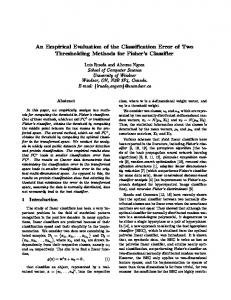
Figure 2: The gallery effect. The algorithm shown here is FI1, but with different galleries (each gallery is a different color).

different color: FI1 (red), FI2 (green), and PCA (blue).

FaceIt Algorithm 1 / 481 Mixed Stratum / 2 PSU

but its spirit is the same). The CMS is a function of an  independent variable r (for rank) and a rank set E — CMS E r  is the fraction of E that has a rank of r or lower. Another view of the CMS is it indicates the fraction of the probes yielded a correct match within the top r candidates. For example, if set E has 256 ranks, 235 of which have a rank of either three or lower, then the value of CMS(E,3) would be 235  256 or 0 918. If we fix E and vary r, the entire set of ranks can be summarized with a single curve. For example, Figure 1 shows the CMS curve for the algorithms FI1 (red), FI2 (green),

3 and PCA (blue) given a particular gallery Q1 and probe set

3 Q2 . There are two fundamental difficulties with interpreting this graph. The first, which can be addressed with our methodology, is that without any sort of standard error it is impossible to determine whether or not one algorithm may have performed significantly better (in the statistical sense). Second, a minor issue, the linear scale compresses the part of the graph we are most interested in — the CMS for the lower ranks. As a metric, the CMS meets our requirement of accurately reflecting information across all of the modes of our conglomerate error distribution. Consider the interaction between the CMS and the multimodal error distribution as we increase the rank. Each point on a CMS curve provides an estimate of how many of the samples were classified correctly as the definition of “correct” changes with the rank. The CMS will have a jump in value as the mode of a class’ error distribution transitions between being incorrect to being correct. If the modes are both broad and numerous, then multiple classes will transition at each increase in rank, and the resulting steps may not be noticeable in the CMS curve. Our first investigation was to determining if changing the training set would have a statistically significant effect on the results. Our initial labeling (i.e., which image of a subject was considered the first, which the second, etc.) was derived directly from the FERET database, and may have caused some degree of homogeneity across the nth image

Cumulative match score

1.00

@

0.90

0.80

0.70

0.60 0.01

0.10 Relative Rank

1.00

Figure 3: Fixing the gallery effect. The algorithm shown here is FI1, but with different mixed galleries (one gallery per color).

available for a given subject. We performed a series of three evaluations, each using one Q 3  as the probe set and the remaining two for the PSUs. The results of this experiment are shown in Figure 2. In this graph, we plot the BRR estimate for each of the three different gallery sets (the thicker, central lines) along with two times their standard deviations (the thinner, bordering lines). The algorithm used was FI1. Like all of the graphs presented in this section, the application of the new methodology required only a single initial training for each set of three curves, not for each point on the curve. So that the graphs may be directly related to confidence intervals, the thin lines correspond to plus or minus two standard deviations. As clearly shown in the graph, the image set corresponding to the top most curve had a (statistically) significantly improved recognition rate. We call this difference the gallery effect. Inferences over evaluations having a dramatic gallery effect, must be made carefully. While conclusions about the population as a whole may be suspicious, the gallery effect may indicate that a particular style of image is favorable for training. For example, in our evaluation, the majority of images of the “best” gallery were of subjects with neutral expressions. Further experimentation may further insight into conditions that are particularly advantageous for face recognition. 6

this particular case (algorithm FI2, 256 stratum, three PSU,

3 gallery Q2 ) the difference among the BRR, bootstrap, and jackknife estimates is particularly dramatic. For the important zero to 0.1 ranks, the BRR provided approximately a 20% decrease in variance. Note, in Figure ?? how the jackknife becomes more and more jagged as the relative rank increases. This may be due to the jackknife’s predisposition against non-smooth statistics. This is also a significant improvement considering that BRR used only 256 replicates, while 768 replicates were used for the jackknife estimate (three PSU + 256 stratum) and 1 000 replicates were selected for the bootstrap estimator. In applications where replicate techniques may be needed for each pixel of an image, using BRR may mean tremendous savings. It is important to reiterate that only rarely will stratification yield less accurate statistics [7]. Naturally, the degree of improvement will vary according to the underlying distribution, its parameters, and the estimated statistic. Figures 6 and 7 are algorithm comparison graphs with errors with one set of three curves per algorithm. Figure 6 was generated with 481 mixed straum with two PSU. Figure 7 was generated with 256 mixed stratum with three PSU. There was some, but not complete, overlap between the data used for different graphs. As shown in the graphs, the PCA algorithm improved so much that it achieved (statistically) similar performance to FI1. Unlike the FaceIt algorithms, the training phase of PCA incorporates information over all subjects by building a low-dimensional subspace that efficiently describes the training data. This improvement may have been due to the fact that a smaller number of subjects were used in this case — 256 instead of 481. Nevertheless, in all four of the graphs, however, we can see that the FI2, for a large portion of all graphs, has a (statistically) significant improvement in recognition rate.

Standard Error of CMS vs. Rank (2 and 3 PSU)

Variance of CMS

0.020

A

0.015

0.010

0.005

0.000 1

10

100 Rank

Figure 4: Comparison of variance between the same 256 strata with 2 PSU (green) and 3 PSU (blue).

Standard Error of CMS (BRR, Jackknife, Bootstrap)

Cumulative match score

0.020

@

0.015

0.010

0.005

0.000 0.01

0.1

1

Rank

Figure 5: Comparison of standard error between BRR (red), jackknife (green), and bootstrap (blue) estimators.

In practice, we cannot guarantee that a subject will take on a particular expression. Therefore, to compensate for the gallery effect, we systematically shuffled the images’ labels, transforming each Q 3 into a set containing an equal fraction of images from each of the original sets. The evaluation was run again, and the results can be seen in Figure 3. As indicated by this graph, mixing the galleries in this manner brought the graphs close enough together, that there was no statistically significant difference between the three curves, strengthening any inference one may decide to make over the context as a whole. For the three PSU case (not shown), mixing brings the curves even closer together. In Section 3.2, it was mentioned that increasing the PSU can reduce the variance in the first-order estimate, and therefore, tighten confidence intervals. In Figure 4, we plot just the variance of the CMS as a function of the rank and PSU with identical strata. The single three PSU case yielded the lowest variance (except for a few anomalies towards the higher ranks). The two PSU cases were each generated by leaving out a single “column” of samples at a time — i.e. only 2  3 of the original data went into the two PSU estimates. As illustrated, the two PSU cases yielded higher variances, especially in the most important low ranks. Figure 5 illustrates the accuracy advantages of using BRR as opposed to traditional jackknife and bootstrapping. For

6. Future Work & Conclusions Like much other work in vision system evaluation, this research has concentrated specifically on algorithm comparison. However, the original motivation of the new methodology was for comparing vision systems that used different sensors. The fundamental difficulty of sensor evaluation is that one cannot insure identical input. That is, given a scene that we wish to image, during a sensor change, there will almost always exist some scene change, regardless of the control the experimenter holds over the environment. Therefore, since non-identical input cannot be guaranteed, single, simple statistics cannot properly reflect the relative merits of the compared sensors; error measures are required to draw evaluatory conclusions with confidence. Potentially, there could be no statistically significant difference between the results yielded by two different sensors within some context, although this may be indicative of a need to add additional constraints to the context. This conclusion would be diffi7

cult to make without any standard error measures. Using the same stratification process provides consistency in such potentially disparate evaluations. In this paper, we presented a new evaluation methodology for the class of vision systems that can be reasonably modeled by a stratified sampling process. We showed how balanced repeated replication can be used to exploit the stratified nature of such evaluations, while simultaneously reducing the amount of required data and computation as compared to bootstrap, jackknife, or cross-validation techniques. We showed how the new methodology could be used to augment the existing FERET [3], [19] evaluation with standard errors and confidence intervals.

CMS vs. rank (2 PSU, 481 mixed strata)

Cumulative match score

1.00

@

0.90

0.80

0.70

0.60 0.01

0.1 Relative rank

1

Figure 6: Mean CMS and error for algorithms FI1 (red), FI2 (green), and PCA (blue) with 2 PSU and 481 mixed strata.

CMS vs. rank (3 PSU, 256 mixed strata)

References Cumulative match score

1.00

[1] Authors. Undisclosed reference. Technical report.

@

[2] Authors. Undisclosed book (to appear), chapter Undisclosed chapter. 2001. [3] D. M. Blackburn, M. Bone, and P. J. Phillips. Facial recognition vendor test 2000. http://www.dodcounterdrug.com/facialrecognition/, Dec 2000.

0.90

0.80

0.70

0.60 0.01

0.1 Relative rank

1

Figure 7: Mean CMS and error for algorithms FI1 (red), FI2

[4] K. W. Bowyer and P. J. Phillips, editors. Empirical Evaluation Techniques in Computer Vision. IEEE Computer Society, 1998.

(green), and PCA (blue) with 3 PSU and 256 mixed strata.

[5] H. I. C. and W. F¨orstner. Performance chateristics of vision algorithms. Machine Vision and App., 9(5–6):215–218, 1996.

[15] D. Krewski and J. N. K. Rao. Inference from statified samples. The Annals of Stat., 9(5):1010–1019, 1981.

[6] K. Cho, P. Meer, and J. Cabrera. Performance assessment through bootstrap. IEEE PAMI, 19(11):1185–1198, Nov 1997.

[16] R. Lehtonen and E. J. Pahkinen. Practical Methods for Design and Analaysis of Complex Surveys. Statistics in Practice. John Wiley & Sons, 1995.

[7] W. G. Cochran. Sampling Techniques. John Wiley & Sons, third edition, 1977.

[17] B. Matei, P. Meer, and D. Tyler. Empirical Evaluation Techniques in Computer Vision, chapter Performance Assessment by Resampling: Rigid Motion Estimators. IEEE Computer Society, 1998.

[8] R. O. Duda, P. E. Hart, and D. G. Stork. Pattern Classification. John Wiley & Sons, second edition, 2001. [9] W. F¨orstner. 10 pros and cons against performance characterization of vision algorithms. In Work. on Performance Char. of Vision Alg., Cambridge, 1996.

[18] P. J. McCarthy. Replication: An Approach to the Analysis of Data From Complex Surveys. U.S. Government Printing Office, Apr 1966.

[10] M. R. Frankel. Inference from Survey Samples: An Empirical Investication. Litho Crafters, Inc., 1971.

[19] P. Jonathon Phillips, Hyeonjoon Moon, Syed A. Rizvi, and Patrick J. Rauss. The FERET evaluation methodology for face-recognition algorithms. IEEE PAMI, 22(10):1090–1104, Oct 2000.

[11] M. Gurney and Robert S. Jewett. Construction orthogonal replications for variance estimation. J. of the American Statistical Association, 70(532):819–821, Dec 1975.

[20] R. L. Plackett and J. P. Burman. The design of optimum multifactorial experiments. Biometrika, 33(4):305–325, June 1946.

[12] R. C. Jain and T. O. Binford. Ignorance, myopia, and naivete in computer vision systems. CVGIP: Image Understanding, 53(1):112–117, Jan 1991.

[21] K. F. Rust and J. N. K. Rao. Variance estimation for complex surveys using replication techniques. Statistical Methods in Medical Research, 5:283–31, 1996.

[13] L. Kish and Martin R. Frankel. Inference from complex samples. J. of the Royal Stat. Soc. B, 36(1):1–37, 1974.

[22] K. M. Wolter. Introduction to Variance Estimation. SpringerVerlag, 1985.

[14] R. Klette, H. S. Stiehl, M. A. Viergever, and . L. Vincken, editors. Performance Characterization in Computer Vision. Kluwer Academic Publishers, 2000.

8