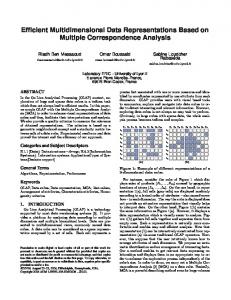
Efficient Multidimensional Regularization for Volterra Series Estimation Georgios Birpoutsoukis, Péter Zoltán Csurcsia, Johan Schoukens Vrije Universiteit Brussel, Department of Fundamental Electricity and Instrumentation, Pleinlaan 2, B-1050 Elsene, Belgium (e-mail:
[email protected]) Abstract: This paper presents an efficient nonparametric time domain nonlinear system identification method. It is shown how truncated Volterra series models can be efficiently estimated without the need of long, transient-free measurements. The method is a novel extension of the regularization methods that have been developed for impulse response estimates of linear time invariant systems. To avoid the excessive memory needs in case of long measurements or large number of estimated parameters, a practical gradient-based estimation method is also provided, leading to the same numerical results as the proposed Volterra estimation method. Moreover, the transient effects in the simulated output are removed by a special regularization method based on the novel ideas of transient removal for Linear Time-Varying (LTV) systems. Combining the proposed methodologies, the nonparametric Volterra models of the cascaded water tanks benchmark are presented in this paper. The results for different scenarios varying from a simple Finite Impulse Response (FIR) model to a 3rd degree Volterra series with and without transient removal are compared and studied. It is clear that the obtained models capture the system dynamics when tested on a validation dataset, and their performance is comparable with the white-box (physical) models. Keywords: Volterra series, Regularization, Cascaded water tanks benchmark, Kernel-based regression, Transient elimination
1. Introduction In the field of system identification, modelling of nonlinear systems is one of the most challenging tasks. One possibility to model nonlinear dynamics in a nonparametric way is by means of the Volterra series ( [1]). The use of the series can be quite beneficial when precise knowledge about the exact nature of the nonlinear system behaviour is absent. Moreover, it has been shown in [2] that a truncated version of the infinite Volterra series can approximate the output of any nonlinear system up to any desired accuracy as long as the system is of fading memory. Practically speaking, it is sufficient that the influence of past input signals to the current system output decreases with time, a property that is met quite often in real systems, such as the cascaded water tanks system considered in this paper. However, it is quite often possible that an accurate nonparametric fitting of nonlinear dynamics requires an excessive number of model parameters. Under this condition, either long data records should be available, resulting in computationally heavy optimization problems and long measurements, or the estimated model parameters will suffer from high variance. This is the reason why the series has in general been of limited use (for echo cancellation in acoustics [3], [4] and for physiological systems [5]), and mostly in cases where short memory lengths and/or low dimensional series for the modelling process were sufficient (e.g. [6]). In the field of mechanical engineering numerous applications of the Volterra series can be found (e.g. for mechanical system modelling [7], [8], [9], for damage detection [10], [11]) . We refer to [12] for an extended survey on the Volterra series and its engineering applications. In this paper, we present a method to estimate efficiently finite Volterra kernels in the time domain without the need of long measurements. It is based on the regularization methods that have been developed for FIR modelling of Linear Time-Invariant (LTI) systems [13], while results exist also for the case of Frequency Response Function (FRF) estimation [14]. In the aforementioned studies, the impulse response coefficients for a LTI system are estimated in an output error setting using prior information during the identification step in a Bayesian framework. The knowledge available a priori for the FIR coefficients was related to the fact that the Impulse Response Function (IRF) of a stable LTI system is exponentially decaying, and moreover, there is a certain level of correlation between the impulse coefficients (smoothness of estimated response). The regularization methods introduced for FIR modelling are extended to the case of Volterra kernels estimation using the method proposed in [15]. The benefit of regularization in this case with respect to FIR modelling is even more evident given the larger number of parameters usually involved in the Volterra series. Prior information about the Volterra kernels includes the decaying of the kernels as well as the correlation between the coefficients in multiple dimensions. Due to the fact that in case of long measurements and higher order Volterra series, the requested memory needs can be more demanding than the available resources, a memory and computational complexity saving algorithm is provided as well. In this work, the regularized Volterra kernel estimation technique is combined with a method for transient elimination which plays a key role in this particular benchmark problem because each measurement contains transient. Due to the fact that the measurement length is comparable to the number of parameters, it is necessary to eliminate the undesired effects of the transient as much as possible. The proposed elimination technique uses a special LTI regularization method based on the ideas of an earlier work on nonparametric modelling of LTV systems [16]. The paper is organized as follows: in Section 2, the benchmark problem is formulated. Section 3 introduces the regularized Volterra kernel estimation method. Section 4 deals with the excessive memory needs of long measurements
and large number of parameters. In Section 5 the proposed method for the transient removal is presented. Section 6 shows the concrete benchmark results showing the efficiency of the combination of the two proposed methods for modelling of the cascaded water tanks system. Early results on the cascaded water tanks benchmark problem can be found in [17]. Finally, the conclusions are provided in Section 7. 2. Problem formulation In this section a brief overview of the benchmark problem is presented. The observed system and its measurements were provided, so the authors and other benchmark performers had no influence on the selection of the measurements. A detailed description of the underlying system, its measurements together with illustrative photos and videos can be found on the website of the workshop [18]. 2.1 Description of the cascaded water tanks The observed system consists of two vertically cascaded water tanks with free outlets fed by the (input) voltage controlled pump. The water is fed from a reservoir into the upper water tank which flows through a small opening into the lower water tank, where the water level is measured. Finally, the water flows through a small opening from the lower water tank back into the reservoir. The whole process is illustrated in Fig. 1. Under normal operating conditions the water flows from the upper tank to the lower tank, and from the lower tank back into the reservoir. This kind of flow is weakly nonlinear [18]. However, when the excitation signal is too large for certain duration of time, an overflow (saturation) can happen in the upper tank, and with a delay also in the lower tank. When the upper tank over flows, part of the water goes into the lower tank, the rest flows directly into the reservoir. This kind of saturation is strongly nonlinear.
Fig 1. Schematic of the underlying system: the water is pumped from a reservoir in the uppertank, flows to the lower tank and finally flows back into the reservoir. The input is the pump voltage, the output is the water level of the lower tank. An illustration of the origin of the transient term in the form of the two dimensional IRF. The dotted IRF refers to the transient. Observe that the transient impulse response function originates before the observation window and its observable (measurable) length is smaller than the LTV impulse responses
2.2 Description of measurement The excitation signal is a random phase multisine [19] with a length ( ) of 1024. The sampling frequency is 0.25 Hz. The excited frequency ranges from 0 to 0.0144 Hz. The Signal-to-Noise Ratio (SNR) is around 40 dB. There are two datasets available for model estimation and validation, respectively. Each measurement starts in an unknown initial state. This unknown state is approximately the same for both the estimation and validation datasets. Furthermore, each dataset contains two overflows at two different time instances. The water level is measured using uncalibrated capacitive water level sensors which are considered to be part of the system. 2.3 The goal This work aims at obtaining a nonparametric time domain model based on the estimation data available. The goodness of the model fit is measured via the validation data on which the RMS error (see (37)) is calculated. The obtained error levels, together with an analysis of the user-friendly method will allow potential users to fairly compare different methods and will motivate them to use the proposed method. 3. The nonparametric identification method 3.1 The model structure It is assumed that the true underlying nonlinear system can be described by the following truncated discrete-time Volterra series [1]:
( ) = ℎ +∑
(∑
…∑
ℎ ( ,…,
)∏
( − ))+ ( )
,…,
,
(1)
where ( ) denotes the input, ( ) represents the measured output signal, ( ) is zero mean i.i.d. white noise with finite variance , ℎ ( , … , ) is the Volterra kernel of order = 1, … , , , = 1, … , denote the lag variables and − 1 corresponds to the memory of ℎ . The Volterra kernels are considered to be symmetric, which means that [12]: ℎ ( ,
,…,
)= ℎ ( ,
,…,
)=⋯= ℎ , ,…,
,
∈ (1, 2, … , ),
,
≠
(2)
∈ (1, 2, … , )
Due to symmetry, it can be easily shown that the number of coefficients to be estimated for a symmetric Volterra kernel = ( )∏ of order ≥ 1 is ( − ). It is also important to clarify the difference between order and degree of ! the Volterra series with an example: the third degree Volterra series contains the Volterra kernels of order 0, 1, 2 and 3. 3.2 The cost function Given input-output measurements from the system to-be-identified, equation (1) can be rewritten into a vectorial , contains vectorised versions of the Volterra kernels =1+ ∑ form as = + , where θ ∈ ℝ , ∈ ℝ contains the measured output and ∈ ℝ ℎ , ∈ ℝ × is the observation matrix (the regressor), contains the measurement noise (observation error).
In this work, the Volterra kernel coefficients in are estimated by minimizing the following regularized least squares cost function as a combination of the ordinary least squares cost function ( ) and the regularization term ( ): =
+
=
+
= |
−
| +
(3)
where the block-diagonal matrix ∈ ℝ × contains ( + 1) submatrices penalizing the coefficients of the Volterra kernels. Given an appropriately structured penalizing matrix (see Section 3.3) and the cost function (3), the regularized least squares solution is given by: =
=(
+ )
(4)
It can be observed that the Maximum Likelihood (ML) estimation of the Volterra coefficients can be computed by setting = 0. The ML estimates suffer very often from high variance in the case of Volterra series estimation due to the large number of parameters in the model (curse of dimensionality). 3.3 Prior knowledge and regularization To overcome the ML estimation issues, a block-diagonal matrix is constructed such that prior information about the underlying dynamics of the true system is taken into account during the identification procedure. The regularization matrix D is constructed using a Bayesian perspective as explained in [20], [21]. It is computed via the product of an ] ( denoting the mathematical expectation operator) and the noise variance inverse covariance matrix = [ as follows: =
(5)
×
is a block-diagonal covariance matrix, = ( , , , … , ) and blkdiag is a function where ∈ ℝ whose output is a block diagonal matrix with the matrix arguments on its diagonal. Each covariance matrix on the diagonal corresponds to a Volterra kernel of different order, namely = [ ] where denotes the vectorised version of the Volterra kernel ℎ .
The matrix introduces the prior knowledge into the cost function as an a priori correlation and scaling between the elements of the IRFs. With respect to the prior knowledge used in this work, it is assumed that the Volterra kernels used to describe the true system are 1) decaying and 2) smooth.
The first property refers to stability not only for the linear term ℎ ( ) but also for the higher dimensional impulse responses (i.e. higher dimensional Volterra kernels). Practically speaking, it is assumed that ℎ ( , … , ) → 0 for , … , → ∞.
The second property of smoothness is related to the correlation between the Volterra coefficients. For the discrete-time Volterra series used in this paper, a smooth estimated Volterra kernel means that there exists a certain level of correlation between neighbouring coefficients, which decreases the larger the distance between two Volterra coefficients.
3.3.1
Kernel-based regression and the covariance matrix
for the first order Volterra kernel
The specific choice of the kernels and the resulting covariance matrix, used to impose smoothness and exponential decaying of the impulse responses, have a major effect on the quality of the estimated model. Note, that the term “kernel” refers to a covariance matrix and is not to be confused with a Volterra kernel. Throughout the paper the word “Volterra” is always used to distinguish between regularization kernels (covariance matrix) and the Volterra kernels in the series (1). 3.3.1.1 Diagonal Correlated (DC) Kernels This kernel has the flexibility to tune independently the properties of smoothness and the exponential decay. The DC kernel function for the first order Volterra kernel (P = [ℎ ( ) ℎ ( ) ]) is defined as follows: (, )=
,
|
| (
)/
(6)
where ≥ 0,0 ≤ < 1, | | ≤ 1. The correlation length between adjacent impulse response coefficients is quantified by (i.e. it controls the smoothness property), and scales the exponential decaying.
Note that in many cases the formulation of the DC kernel differs from (6), like in [22] but the expressions are equivalent. 3.3.1.2 Tuned-Correlated (TC) Kernels While the DC kernel gives a nice flexibility to tune the model behaviour, unfortunately it can lead to a very high computational complexity (3 parameters to tune). In some cases TC kernels – as a special form of DC – can provide a good balance between the flexibility and the computational load. When, in the DC kernel structure, is set equal to √ then it leads to the TC form: ,
(, )=
where
(, )
(7)
≥ ,0 ≤ α < 1.
Note, that the TC kernels are widely used in different regularization toolboxes (e.g. ident in Matlab). 3.3.1.3 Other kernels Depending upon the prior knowledge, different covariance matrices can be used as well. This holds true also for the higher order Volterra kernels (see next). A detailed comparison can be found in [13], [23], [24]. 3.3.2
The covariance matrix
for the second order Volterra kernel
The two facts of decaying (stability) and smoothness (correlation) for the second order Volterra kernel are encoded into the matrix (see (2)) using the method described in [15]. It is an extension of the regularization methods for linear impulse response [25] using the Diagonal Correlated (DC) kernel (again not to be confused with a Volterra kernel) to higher dimensions such that prior information is imposed to a multi-dimensional impulse response. The properties of decaying and smoothness for the 2nd order Volterra kernel are encoded into the matrix P . The ( , )element, which corresponds to , is given by [15]: , , ∀ , where , , , denote two Volterra coefficients in
Fig 2. Left: An example of a smooth and exponentially decaying second order Volterra kernel. Right: X-Y view of the same Volterra kernel together with the two directions, along which prior information is imposed.
,
(, )=
|
|
|
|
(8)
- coordinate system is rotated 45 degrees counter-clockwise with respect to the coordinate system t1 and t 2 (see Fig.2, right): where the
=
,
cos(45 ) −sin(45 ) sin(45 ) cos(45 )
,
(9)
,
The so-called hyperparameters and are used to control the correlation between the coefficients along the and direction, respectively. The hyperparameters and determine the decay rate along the and direction, respectively. Hyperparameter is a scaling factor used to determine the optimal trade-off between the measured data and the prior information encoded in (the subscript 2 is used in to show that this hyperparameter is different from used in (6)–(7) for the first order Volterra kernel and in general different for every Volterra kernel in the series). Equation (8) can also be seen as the product of two DC kernels applied in the and directions, respectively. For a more detailed analysis on the proposed covariance matrix for the second order Volterra kernel, the interested reader is referred to [15]. 3.3.3 Extension of the method to higher order Volterra kernel estimation The Volterra kernel regularization method proposed for the second order Volterra kernel can be extended to cover the case of Volterra kernels of orders higher than two. In Fig. 3 a part of the third order kernel, described by the function ℎ ( , , ) in the Volterra series (1), is depicted. Each sphere corresponds to a different value of the function ℎ (different point). The diagonal direction is now given by the blue arrow with orientation (1,1,1) (in the , , coordinate system).
Fig 3. The three directions, along which prior information is imposed, for the third order Volterra kernel.
At each point on this direction, there corresponds a plane described by the equation + + = . In Fig. 3 these planes are delimited with green lines. Following the same reasoning as for the second order kernel, two extra directions are needed, in order to describe the prior knowledge of exponential decaying and smoothness on each of these planes. Therefore, the three directions (orientation (1,1,1)), (orientation (1,-1,0)) and (orientation (-1,-1,2)) can be used to formulate the covariance for the three dimensional impulse response, following the same reasoning as in (7). In this way, the concept of imposing prior information through regularization can be further extended to higher dimensional Volterra kernels. 3.4 Tuning of the hyperparameters All the so-called hyperparameters, such as , , in , , , , , in as well as (noise variance) and = [ℎ ∙ ℎ ] are tuned with the use of the input and output data used for estimation. The nonparametric system identification method presented in this work consists essentially of two steps: ·
Optimization of the hyperparameters to tune the matrix
·
Computation of the model parameters (Volterra series coefficients) using (4).
(and further
in (5)).
The values of the hyperparameters can be tuned in many different ways. The theoretical aspects of the possible optimization techniques are beyond the scope of this paper. In this work the marginal likelihood approach [26], [27] and a residual analysis [28] are used because they need only one (estimation) dataset for the entire estimation procedure.
However, it is important to point out that a simple cross-validation technique [19] can be used as well, but it would not fall within the frames of the measurement benchmark problem since it would also require the use of the validation dataset. 3.4.1 The marginal likelihood approach The hyperparameters are optimized in this case by maximizing the marginal likelihood of the observed output, which boils down to: = arg min
Σ
+
Σ
(10)
where is a vector containing all the hyperparameters and Σ = ( + ) ∈ ℝ × represents the covariance matrix of the output vector , and denotes the identity matrix. Practically speaking, the optimal set of hyperparameters given the measured output data determines the covariance matrix which is most likely to have generated the observed output. The objective function (10) is non-convex in , therefore to minimize the risk of resulting in a local minimum, it is advised that multi-start optimization of the hyperparameters is performed. 3.4.2 The residual analysis approach In case of residual analysis [28] the hyperparameters, the model and the measured outputs are analysed simultaneously. The output simulation is performed by using a set of (candidate) hyperparameters as = , see (1),(4). In this terminology the residuals ( ) are the differences between the simulated output and the measured output, i.e. = − .
It can be clearly seen that the residuals represent a part of the data that are not explained by the model. In practice, the residual analysis consists of two tests: the whiteness test and the independence test. If the residuals are white and independent of each other, then an appropriate model order as well as set of hyperparameters has been retrieved. The interested reader can refer to [29] for more techniques for the tuning of the hyperparameters. 3.4.3 Computational concerns
The inversion of Σ in (10) for the marginal likelihood maximization, which is equivalent to the one in (4) for the residual analysis approach, is performed multiple times during the optimization of the hyperparameters. This matrix inversion constitutes one of the most time-consuming parts of the nonparametric identification method presented in this paper due to its large size (Σ ∈ ℝ × ). In the following section, the problem of matrix inversion both at the level of the cost function as well as at the level of the hyperparameters optimization is tackled. 4. Coping with large datasets and excessive number of parameters 4.1 Introduction In the past, engineers and scientists barely used Volterra models for nonparametric estimation due to the fact that it required 1) much more measurement samples than the number of model parameters, and 2) an excessive number of parameters. Injecting prior information, such as smoothness and decaying, decreases significantly the need for long data records. Further, there is a significant increase at the modelling quality due to the injection of prior knowledge, however, this is at the price of increased computational complexity and higher memory needs. The computational complexity increases with the degree of the Volterra series (and thus with the increasing number of parameters, see Fig. 4).
Fig 4. The number of model parameters up to the fourth order symmetric Volterra kernel is shown as a function of the memory length (truncation lag).
The exact computational time depends on many factors such as the model complexity, the way how the matrix algebra is implemented, the initial values of the hyperparameters, and the technique used to tune the hyperparameters. A
significant amount of time can be saved by using different hyperparameter optimization strategies, and by choosing properly the initial values. The case of hyperparameter tuning using the Marginal Likelihood approach when the data length is much larger than the number of parameters has already been studied in [29]. However, this is not the case of the cascaded water benchmark problem (see Section 2.2 and Section 6.4). In general, the most time-consuming part is the matrix inversion in (4) which needs to be executed in each optimization cycle of the tuning of hyperparameters. Another (hidden) matrix inversion problem can be found in the penalization matrix ∈ ℝ × . In general, the numerical values of are computed via scaled and inverted covariance matrices.
A further highly related issue is the exaggerated memory needs. In general, when LTI systems are identified by regularization technique, the memory needs are quite limited. However, considering the matrix sizes in this particular case, it can be clearly seen that by increasing the length of the measurement, the requested operational memory size grows linearly as (2 × + ), by increasing the number of parameters it grows quadratically as (3 × + ). Further, the memory needs also grow as a power function of the number of lags to the Volterra degree i.e. ), see Fig 4. (∑
In order to illustrate the problem an example is given. Let us assume that a nonlinear system is modelled with the third degree Volterra model, the measurements contain 10 000 samples, the number of lags in the first and second order Volterra kernels is 100, the number of lags in the third order Volterra kernel is 50. In this case the requested memory size (with 8 byte floating precision) is more than 459 GB RAM. However, most of the personal computers do not have this capacity, therefore a solution is needed which would allow to run a higher degree Volterra kernel estimation on every (modern) computer. 4.2 Proposed solution In this work a vectorised gradient based method is presented. By applying the proposed technique it is possible 1) to avoid the inversion in the regularised LS solution (4), 2) to avoid the inversion in the penalization matrices (5), and 3) to reduce the memory needs. It is important to remark that in [16] regularized two-dimensional IRFs were studied where one faced very similar memory issues presented here. The key idea of [16] is that instead of computing the 2D timevarying nonparametric model in one step for a large dataset, a special sliding window can be used for partial datasets resulting in a smaller computational load. The sliding window is applied over different, consecutive impulse response functions. Unfortunately, due to the problem formulation this technique cannot be applied here. 4.3 Avoid inversion in the cost function At this point it is important to recall the original cost function (3). The exact solution of the regularized estimate – for a set of hyperparameters encoded in – is given by (4). The inversion in (4) needs to be (re)calculated for each set of hyperparameters –in each hyperparameter optimization cycle. In order to avoid inversion of large matrices (i.e. in case of large ), it is advised to use an inversion-free gradient based method. In order to obtain the proposed algorithm, first let us calculate the gradient of the cost function (3): =
(
+
)=
(‖
−
‖ +
)=
(
+
)=−
Next, let us introduce new terms for the proposed method. The Jacobian ( ∈ ℝ × ( ∈ℝ ) matrices are defined as follows: =
[
=[
]
] = [−
]
×
+
(11) ) and gradient descent direction (12) (13)
In the proposed gradient based method several iterations –i.e. updates– will be needed. The actual iteration number is indicated hereinafter in the subscript of the variables. The initial value of the parameter estimate vector ( ) is advised to be set to zero. At ( + 1)th step, the new value of the parameter estimate is given by: =
where
(14)
−
∈ ℝ is used as a weighting factor for the gradient descent direction.
Using the above-mentioned terms, for a given penalization matrix , the algorithm of the inversion-free regularized solution is the following: 1.
Initialize
2.
Calculate the initial cost function
3.
Repeat until the maximum number of iterations is reached:
.
a) Compute the descent direction (
= (
).
) and initialize .
b) Calculate the new candidate value of the parameter estimate vector ( c) If |
−
e) If
| is smaller than the tolerance level of the cost function change, then leave 3.