Efficient Multiple Feature Fusion with Hashing for ...

IEEE TRANSACTIONS ON GEOSCIENCE AND REMOTE SENSING

1

Efficient Multiple Feature Fusion with Hashing for Hyperspectral Imagery Classification: A Comparative Study Zisha Zhong, Bin Fan, Member, IEEE, Kun Ding, Haichang Li, Shiming Xiang, and Chunhong Pan, Member, IEEE

Abstract—Due to the complementary properties of different features, multiple feature fusion has a large potential for hyperspectral imagery classification. At the meantime, hashing is promising in representing high dimensional float type feature with extremely low-bits binary codes while maintaining the performance. In this paper, we study the possibility of using hashing to fuse multiple features for hyperspectral imagery classification. For this purpose, we propose a multiple feature fusion framework to evaluate performance of using different hashing methods. For comparison and completeness, we also have an extensive comparison to five subspace-based dimension reduction methods and six fusion-based methods which are popular solutions to deal with multiple features in hyperspectral image classification. Experimental results on four benchmark hyperspectral data sets demonstrate that using hashing to fuse multiple features can achieve comparable or better performance with the traditional subspace-based dimension reduction methods and fusion based methods. Moreover, the binary features obtained by using hashing need much less storage and are faster to compute distances with the help of machine instructions. Index Terms—Feature fusion, Hashing, Binary codes, Hyperspectral images, Classification

I. I NTRODUCTION Hyperspectral imaging technology provides us spectral signatures with a large number of bands [1], [2], significantly characterizing the inherent physical and chemical properties of imaged objects [1], [3]. However, it turns out to be very challenging for hyperspectral image processing because of the high dimensionality of pixels resulting from the increased spectral resolution [4]. Consequently, it attracts more and more interests in remote sensing and other research communities such as machine learning and computer vision [5]. As a vital application of hyperspectral images, land-cover classification which aims at classifying image pixels into multiple categories remains an active research area [6] [7]. Manuscript received April 28, 2015; revised October 04, 2015 and February 14, 2016; accepted February 29, 2016. Date of publication XXXX XX, XXXX; date of current version XXXX XX, XXXX. This work was supported in part by the Projects of the National Natural Science Foundation of China (Grant No. 61573352, 61472119, 91338202, 91438105) and the Beijing Natural Science Foundation (Grant No. 4142057). Z. Zhong, B. Fan, K. Ding, H. Li, S. Xiang, C. Pan are with the National Laboratory of Pattern Recognition, Institute of Automation, Chinese Academy of Sciences, Beijing, China (e-mail: {zszhong, bfan, kding, hcli, smxiang, chpan}@nlpr.ia.ac.cn). Color versions of one or more of the figures in this paper are available online at http://ieeexplore.ieee.org. Digital Object Identifier 10.1109/TGRS.2016.XXXXXXX

Recent studies [2], [4], [8] have demonstrated that the joint exploitation of both spectral and spatial information can significantly improve the classification accuracy. To sum up, there are mainly three kinds of spectral-spatial algorithms for hyperspectral imagery classification [4]: (1) spectral-spatial feature extraction, (2) spatial-spectral segmentation [9]–[12] and (3) other methods (e.g., kernel-based [13]–[15] and Markov random field methods [16]). In terms of spectral-spatial feature extraction, lots of endeavors have been devoted to develop effective and efficient feature extraction algorithms to improve hyperspectral imagery classification. Representative techniques include filteringbased methods (e.g., Gabor filtering [17], edge-preserving filtering [18]), morphology-based methods (e.g., extended morphological profiles (EMP) [19], extended attribute profiles (EAP) [20], [21]) and spatial statistical feature extraction (e.g., gray-level concurrence matrices [22], [23]). These methods can achieve significant improvement on classification performance. Since single kind of feature only carries some certain characteristics of the object, some researchers designed feature fusion approaches to integrate multiple types of features for further improving the classification performance. Recent advances on multiple feature fusion can be divided into four categories: multiple kernel learning methods, subspace-based feature extraction methods, feature selection based methods and ensemble methods. Most multiple kernel learning methods have been focused on the effective or efficient composition of different kernels [5], [24]–[27]. Li et al. [15] have developed a framework to integrate multiple types of features extracted from both linear and non-linear transformations without the need to learn the weights of considered features. Gu et al. [28] have proposed a representative multiple kernel learning approach for efficiently determining the optimal kernels in hyperspectral image classification. Considering the subspace-based methods, Zhang et al. [29] have proposed a multiple feature combining approach to encode different features into a low-dimensional representation based on manifold learning and patch alignment framework [30]. Additionally, Zhang et al. [31] have introduced a modified stochastic neighbour embedding algorithm for multiple feature dimension reduction under a probability-preserving projection framework. Unlike the feature extraction methods, feature selection does not create new feature representations and can keep the physical meanings of features, thus attracting great interest of researchers. A very recent study on multiple feature


selection is [32], in which a discriminative sparse multimodal learning is developed for multiple feature selection. By introducing a structured regularization technique, they have extended the original discriminative least square regression framework [33] to exploit both the intrinsic structures in data and the correlations among different features. Different from the above methods, an SVM ensemble fusion method has been proposed in [34] that construct a support vector machine (SVM) ensemble to combine multiple spectral and spatial features at both pixel and object levels. The existing methods for multiple feature fusion are mainly focused on improving their classification accuracy without considering the computational and storage cost. However, with the increasing demand of earth observation and with the development of hyperspectral imaging technology, we can obtain more and more high-quality hyperspectral images with higher and higher spectral resolution. Thus, we are facing the challenge of processing these huge amount of data. As a result, it requires efficient solutions for hyperspectral imagery classification, both in processing time and memory footprint. Unfortunately, there are few literatures dealing with this problem. As a powerful technique to obtain compact features and fast nearest neighbor search, hashing has not been introduced in remote sensing processing until very recently [35], where it is adopted for large scale remote sensing image retrieval. To the best of our knowledge, it has not been used in hyperspectral image classification. In this paper, we introduce using hashing technique to extract compact binary features for hyperspectral image classification in the proposed multiple feature fusion with hashing (MFH) framework. To show the effectiveness of using hashing technique in this task, we give a comparative study on applying different hashing techniques to generate compact binary codes. Based on the extensive experimental evaluations on four standard hyperspectral data sets, we discuss advantages and disadvantages of using hashing for fusing multiple features. The main contributions of our work are summarized as follows: 1) We propose a multiple feature fusion with hashing (MFH) framework to use hash technique in fusing multiple features for hyperspectral image classification and show encouraging results. 2) We conduct an extensive performance evaluation of different hashing methods on fusing multiple features for classification on four popular hyperspectral data sets. Based on the evaluation results, we supply with an indepth discussion on the advantages, disadvantages and availability of different hashing methods in this task. 3) We conduct comparative experiments with five classical subspace-based dimension reduction methods and six different multiple feature fusion methods. Experiments show that when equipped with a proper hashing learning strategy, the proposed MFH method can achieve comparable or even competitive performance. Meanwhile the obtained binary features require much less storage and classification time. The rest of this paper is organized as follows. Section II introduces the proposed MFH framework. Section III gives

2

a brief introduction of six representative hashing algorithms adopted in MFH, including three unsupervised ones and three supervised ones. Section IV describes the four used data sets and elaborates our experimental setups as well as evaluation protocol. Section V presents the experimental results and analysis. Then, we give an overview and guidelines for potential users based on our experimental observations in Section VI. Finally, Section VII concludes this paper with some possible future works. II. T HE MFH

FRAMEWORK

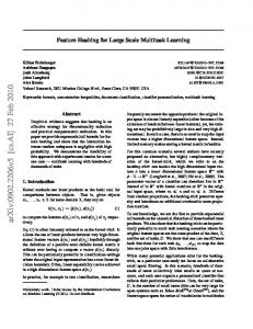
The proposed MFH framework can be divided into three steps: 1) perform feature extraction in the hyperspectral image via efficient approaches and concatenate multiple features into a long feature vector for each pixel; 2) perform hashing learning on these feature vectors with or without class label information and map the original float-type feature vectors into compact binary codes; and 3) perform classification with the obtained binary codes and output the final classification results. The flowchart of MFH is shown in Fig. 1. In the following, we will describe these three steps in detail. A. Multiple Feature Extraction Feature extraction plays a very important role in pattern recognition. In remote sensing society, a lot of research endeavours have been devoted and much efficient feature extraction methods have been developed. Owing to these works, different types of features can be extracted from the hyperspectral image. Without loss of generality, suppose N kinds of features are extracted for each pixel i. Then, we stack N these features into a long vector xi = {xik }k=1 ∈ R1×D , 1×dk where xik ∈ R is the k-th single feature descriptor ∑N for pixel i and dk is the dimension of the feature. D = i=1 dk is the length of the fused feature descriptor. B. Hashing Learning Hashing aims at mapping the original data into compact binary codes, or equivalently a sequence of bits, while preserving similarity in the original data space [36]–[38]. Due to the binary characteristic, their distances can be computed extremely fast with Hamming metric in modern computers, which consequently facilitates faster nearest neighbor search. Meanwhile, storing binary codes requires much less memory footprint compared to storing float vectors. Specifically, given n training samples {xi , yi }ni=1 where xi ∈ R1×D is the i-th training point with D float-type features, yi ∈ {1, · · · , C} is the class label of i-th training point and C is the number of labeled classes. The hashing B learning is to learn a set of hashing functions {hb (x)}b=1 to map the original high-dimensional float-type feature xi ∈ R1×D (i = 1, · · · , n) into a low-dimensional binary code zi ∈ {−1, 1}1×B where B ≪ D is the number of bits used and the b-th bit of zi is the output of hb (xi ). Once the hashing functions are learned, the fused float-type multiple feature vectors extracted in a hyperspectral image can be encoded into binary codes and be given as inputs for the following classification procedure.


3

Multiple feature extraction

Binary codes

‫ݔ‬ଵ ‫ݔ‬ଶ

… Feature 2 Z

…

Unlabeled samples Learned hash functions

Feature 1

‫ݖ‬ଵ 0 1 0 1 0 0 0 1

‫ݖ‬ଶ 1 1 1 1 0 0 1 1

…

…

…

Hashing Learning

Feature i

1-NN Classification With Hamming metric

… …

…

…

Labeled samples

Feature N Training samples

…

Fig. 1.

Classification map

Flowchart of the proposed MFH framework.

C. Classification with Binary Codes Finally, based on class label, these compact binary codes are given as inputs for nearest neighbor (1-NN) classifier with Hamming metric to predict the class labels and output the classification results. III. F EATURE H ASHING In the proposed MFH framework, the classification performance would largely depend on the quality of binary codes obtained by hashing methods. As a consequence, a key problem is to design good schemes for finding good binary codes. Fortunately, there are a lot of theoretic or practical efforts in literature on solving this problem from various viewpoints [36]–[38]. According to whether the label information is used or not, we roughly divide the existing hashing methods into two categories: unsupervised and supervised ones. Unsupervised hashing methods try to preserve the distance-based similarity in original feature space, while the supervised ones are developed to preserve the labelbased similarity. In this section, we will briefly introduce three representative hashing methods for both categories, respectively. And in the following sections, we will adopt them in the proposed MFH framework and give a detail evaluation on the classification performance on four popular hyperspectral data sets. A. Locality Sensitive Hashing (LSH) LSH is one of the basic but most popular hashing methods. Given a data point x ∈ RD , for the b-th bit of the binary code, a random vector wb ∈ RD is selected from a zero-mean Ddimensional normal distribution N (0, ID ), ID is an identity matrix, and the hashing function is defined as: { 1, if wbT x ≥ 0 hb (x) = −1, if wbT x < 0.

Both [39] and [40] have proved that the random projections can preserve similarity as the number of hash bits increases, and meanwhile, they have also observed that the number of required hash bits may be large for high-dimensional data. LSH is totally probabilistic and does not take the data distribution into account, so its performance is limited. However, for its simplicity, LSH is popular and usually served as baseline for performance comparison in hashing. B. Kernalized Locality Sensitive Hashing (KLSH) The KLSH proposed by Kulis et al. [41] generalizes LSH by using kernel technique, which makes it possible to embed high-dimensional features or complex distance functions into a low-dimensional Hamming space. The main idea of KLSH is to approximate the Gaussian-based random projections in the kernel space by using a weighted combination of kernelmapped anchors selected from the input space, based on the central limit theorem [42]. Specifically, given an arbitrary kernel function κ (xi , xj ), the main steps are as follows: 1) Select p data points from the input space and form a kernel matrix K upon them. 2) Center the kernel matrix K. 3) For each hash function hb (ϕ (x)), form a indicator vector eS by randomly selecting t indices from [1, · · · , p], then form wb = K−1/2 ∑epS , and generate a bit according to hb (ϕ (x)) = sign ( i=1 wb (i) κ (x, xi )). Here, sign(·) is a sign function. As stated in [41], KLSH is simple with general applicability and usually preferable in cases where the computation of the hash functions is dependent on the kernel embeddings. ( ) However, the computation of K−1/2( has O p3 time ) complexity, the computation of wb has O p2 time complexity and with the obtained wb , the final hb (ϕ (x)) needs O (p) time complexity. As a consequence, it is suggested that p should be much smaller than n in order to maintain efficiency [41].


C. Spectral Hashing (SH) Weiss et al. [43] have formalized the problem of finding hashing functions as graph partition and developed a solution based on spectral relaxation where the hash bits are calculated by thresholding a subset of eigenvectors of the Laplacian of the similarity graph. Specifically, the optimization criterion is to minimize the average Hamming distance between similar items, which is formulated as follows: ( ) min trace ZT LZ s.t.

ZT 1n = 0,

ZT Z = In

where trace(·) is trace operator, Z ∈ {−1, +1}n×B is the binary codes for training samples and L is the graph Laplacian in original space. In is an identity matrix with n rows. The constraint of ZT 1n = 0 is to assure that each bit of these binary codes should have equal number of −1 and +1. 1n ∈ Rn is a all-one vector. The constraint of ZT Z = In means that the hashing bits are uncorrelated to each other. The above optimization is solved by relaxing Z to continuous values and the final binary codes are obtained by thresholding Z. By utilizing recent results on convergence of graph Laplacian eigenvectors to the Laplace-Beltrami eigenfunctions of manifolds, they have also showed how to efficiently calculate the binary code of a testing sample. As reported in [43], SH has two limitations. The first is the assumption of a multidimensional uniform distribution of the data, which usually does not hold in real cases. The second is the eigenvalues from the outer-product eigen-functions are discarded to maintain the uncorrelatedness of bits, which would break the uncorrelated property when there are more than one eigenfunction along a single PCA direction and consequently result in a deteriorated performance [37]. D. Kernel-Based Supervised Hashing (KSH) Liu et al. [44] have proposed a novel kernel-based supervised hashing model in which the supervised information comes from similar and dissimilar data pairs. The idea is to map the original data to compact binary codes whose Hamming distances are minimized on similar pairs and simultaneously maximized on dissimilar pairs. By utilizing the algebraic equivalence between Hamming distance and inner product, they designed an efficient greedy algorithm to learn the hashing functions one by one. To deal with linear inseparable data, the kernel-based hash functions are adopted, which are defined as )[41] hb (x) = (∑ ( ) m sign (f (x)) = sign j=1 κ x(j) , x aj − c , where c = ( ) ∑n ∑m aj i=1 j=1 κ x(j) , xi n , m is the number of uniformly selected anchor samples for kernel computation, aj ∈ R is the coefficient and c is the bias. After simplifying the notion, ¯ (x) where a = [a1 , · · · , am ]T and we obtain f (x) = aT k [ ( ) ( ) ] ¯ (x) = κ x(1) , x − µ1 , · · · , κ x(m) , x − µm T k ( ) ∑n where µj = n1 i=1 κ x(j) , xi . Different from KLSH where the coefficient vector is the random projection constructed based on the subset of data samples, here, the vector a is optimized by leveraging supervised information which

4

results in more discriminative hashing functions. Specifically, considering B hash bits, the problem is to find B coefficient vectors a1(, · · · , aB)}to construct B hashing functions { ¯ (x) B . Since directly optimizing on hb (x) = sign aTb k b=1 Hamming distance is nontrivial, the authors deduced an equivalence between inner product and Hamming distance: code (xi ) ◦ code (xj ) = B − 2Dh (xi , xj ), where Dh (xi , xj ) is the Hamming distance between the binary codes of xi and xj . Based on this relationship, the optimization problem is modeled as 2 1 T min Q = Hn Hn − S (1) n×B B Hn ∈{−1,+1} F   code (x1 )  ··· where ||·||F is the Frobenius norm and Hn =  code (xn ) denotes the binary code matrix for the n training samples, code (x) is the binary code of x, and the label matrix S records the pairwise relationship, where   (xi , xj ) ∈ M 1, Sij = −1, (xi , xj ) ∈ C   0, otherwise and M is the set of similar pairs, C is the set of dissimilar pairs. Then, with some simple operations, the code matrix Hn can be rewritten as   h1 (x1 ) , · · · , hB (x1 ) ( )   .. .. .. ¯ nA Hn =   = sign K . . . h1 (xn ) , · · · , hB (xn ) [ ] ¯ (x1 ) , · · · , k ¯ (xl ) T ∈ Rn×m and A = ¯n = k where K [a1 , · · · , aB ] ∈ Rm×B . Then substitute Hn into Eqn. (1), the final objective is to minimize 2 1 ( )( ( ))T ¯ ¯ Q (A) = sign Kn A sign Kn A − S . B F Based on the separable property of code inner products, a greedy optimization is proposed to obtain the hashing function for each bit one by one. Finally, with the obtained coefficient vectors [a∗1 , · · · ,[a∗B ], the xi ) for a testing ( T sample )] ( Tbinary code ¯ (xi ) a∗ , · · · , sign k ¯ (xi ) a∗ . is computed by sign k 1 B Owing to the class label based similarity-preserving objective, KSH can yield short yet discriminative codes. E. CCA-based Iterative Quantization The iterative quantization (ITQ) [45] is proposed to find a rotation transformation of data by minimizing the quantization error between the PCA-reduced data and binary codes. Originally, ITQ is developed to learn binary codes unsupervisedly. It consists of two steps: 1) apply PCA to the original data X ∈ Rn×D : V = XP ∈ Rn×B , where P ∈ RD×B (B ≤ D) is the PCA projection matrix; 2) find the binary codes Z ∈ {−1, +1}n×B along with an optimal rotation matrix R based on the PCA-reduced data V by minimizing the quantization loss 2

Q (Z, R) = ||Z − VR||F .


5

The problem is solved via two-step alternative optimization. The first step is to update Z by Z = sign (VR) with the fixed R. The second step is to update R with the fixed Z by solving a standard orthogonal Procrustes problem. For testing samples, the obtained R is also used to transform their PCA-reduced features into binary codes. When label information is available, the PCA can be replaced with canonical correlation analysis (CCA) [46], resulting in the CCA-based ITQ algorithm (CCAITQ). As shown in [45], the CCA-ITQ is very effective and can significantly improve the performance of image retrieval. F. FastHash Lin et al. [47], [48] have proposed a flexible yet simple supervised hashing framework that is able to accommodate different types of loss functions and hash functions. Their work consists of two steps: binary code inference and hashing function learning. The first step is formulated as binary quadratic programming that is proved to be block-submodular and consequently the graph cut technique is used for efficient solution. In the second step, the boosted decision trees are adopted as supervised hashing functions that can be very fast to train and evaluate on large-scale high-dimensional data. More specifically, the authors first formulated the hashing learning problem as n ∑ n ∑ min δ (yij ̸= 0) L (Φ (xi ) , Φ (xj ) ; yij ) (2) Φ(·)

i=1 j=1 B

where Φ (x) = [h1 (x) , · · · , hB (x)] ∈ {−1, +1} is the binary code for data point x. δ (·) is the indicator function, and δ (yij ̸= 0) ∈ {0, 1} indicates whether the relation between two data points is defined, yij = 1 indicates xi and xj are similar and yij = −1 designates dissimilar. L (·) is a loss function that measures how well the binary codes match the ground truth similarity yij . By introducing auxiliary variables zi,b = hb (xi ) ∈ {−1, +1} as the output of the b-th hash function on xi , the problem in Eqn. (2) is decomposed into two subproblems: n ∑ n ∑ min δ (yij ̸= 0) L (zi , zj ; yij ) Z

i=1 j=1 n×B

Z ∈ {−1, +1} and min Φ(·)

B ∑ n ∑

δ (zi,b = hb (xi ))

b=1 i=1

where zi = [zi,1 , · · · , zi,B ] is the binary code for xi . The B hash functions are solved one by one. For each hash function, the two subproblems are solved alternatively. After solving for one bit, the binary codes are updated by applying the learned hash functions. As a result, the learned hash function can influence the solution of the following bits. For the binary code inference of the b-th hash bit, let the binary codes of the previous (b − 1) bits be fixed, the problem is simplified as n ∑ n ∑ min (3) δ (yij ̸= 0) lb (zi,b , zj,b ; yij ) z(b)

i=1 j=1

n

where z(b) = [z1,b , z2,b , · · · , zn,b ] ∈ {−1, +1} is b-th bit values of the binary codes of the n training samples. lb represents the loss function output for the b-th bit, conditioning on the previous (b − 1) bits: ( ) (r−1) (r−1) lb (zi,b , zj,b ; yij ) = L zi,b , zj,b ; zi , zj , yij (r−1)

where zi represents the binary code of xi in all previous (b − 1) bits. It has been proved that the problem in Eqn. (3) can be rewritten into a standard binary quadratic optimization problem with any Hamming affinity or distance based loss function L (·), and several different loss functions L (·) were discussed [48]. Then, a graph cut based block search method is developed for efficient solutions in large-scale problems. For the second step, hashing function learning is to solve a binary classification problem for learning one hash function. The binary codes obtained in the first step are used as the classification labels. Any binary classifiers can be directly applied. To effectively deal with high-dimensional nonlinear data, the boosted decision trees are adopted. Finally, the hash function is defined as a linear combination of decision trees: [ Q ] ∑ hb (x) = sign (4) wq Tq (x) q=1

where Tq (·) ∈ {−1, +1} denotes q-th decision tree with binary output and Q is the number of decision trees, wq is the weighting coefficient, which can be solved by Adaboost. As shown in [48], since FastHash adopts the boosted decision trees as the hash functions which can effectively and efficiently deal with high-dimensional nonlinear data, it can generate highly descriptive binary codes. IV. E XPERIMENTAL S ETUPS In this section, we present an experimental evaluation to test the performance of the proposed MFH framework for hyperspectral imagery classification. Section IV-A shows the used four standard benchmark hyperspectral data sets. Section IV-B simply introduces four well-known feature extraction methods that are used to generate the multiple feature vectors for fusion. Section IV-C describes the evaluated methods and their parameter settings. Finally, section IV-D defines the evaluation criterions for experimental analysis. A. Data Sets Indian Pines: this data set was captured by the Airborne Visible/Infrared Imaging Spectrometry (AVIRIS) sensor over a mixed agricultural/forested region in Northwest Indiana, on June 12, 1992. This data set has a spatial size of 145 × 145 pixels and 220 spectral bands with a spatial resolution of 20 m/pixel. It has 16 land-cover classes, whose sizes of labeled samples disproportionately range from 20 to 2468 pixels. In the experiments, we remove 20 noisy bands (104–108, 150–163, and 220) due to water absorption and use the remaining 200 bands. The false color and its ground truth images are shown in Fig. 2. University of Pavia: this data set was acquired by the Reflective Optics System Imaging Spectrometry (ROSIS),


(a)

(b)

6

(c)

Fig. 2. (a) False color image of Indian Pines data set, (b) its ground truth image and (c) its labeled classes.

covering an urban area of the University of Pavia, Italy. Originally, the ROSIS sensor provided 115 bands from 0.43 to 0.86 µm. After removing the 12 most noisy bands, the remaining 103 bands are used for experiments. The spatial size of this data set is 610 × 340 pixels, and its spatial resolution is 1.3 m/pixel. There are 9 classes, with sizes of labeled samples ranging from 1026 to 18686. The false color and its ground truth images are shown in Fig. 3.

(a)

(b)

(c)

(d)

Fig. 3. (a) False color image of University of Pavia data set, (b) its ground truth image, (c) the given training samples and (d) its labeled classes.

Salinas: this data set was captured by the AVIRIS sensor over Salinas Valley, California, with a spatial resolution of 3.7m/pixel. This data set has a spatial size of 512 × 217 with 224 spectral bands. In our experiments, 20 water absorption bands (108 − 112, 154 − 167, and 224) are discarded. This data set has 16 classes, whose sample sizes range from 916 to 11271. The false color and its ground truth images are shown in Fig. 4.

(a)

(b)

(c)

Fig. 4. (a) False color image of Salinas data set, (b) its ground truth image and (c) its labeled classes.

Houston: this data set was initially distributed in the 2013 IEEE Geoscience and Remote Sensing Data Fusion Contest [49], [50], which includes an urban hyperspectral data set and a Light Detection And Ranging (LiDAR) derived digital surface model. Both are geographically referenced and at the same spatial resolution (2.5 m). The hyperspectral data set has 144 bands in the 380–1050 nm spectral region. There are 15 classes of interest selected by the organizers. Fig. 5 shows the false color image of hyperspectral data, the colored LiDAR image and the given training and testing samples. For these four data sets, the number of training and testing samples for each class will be described in their respective experimental section.

B. Multiple Feature Extraction Four kinds of commonly-used features in hyperspectral image processing are extracted for each pixel, including: (1) the original spectral feature (denoted as Spectral), (2) the extended morphological profiles feature (denoted as EMP) [19], (3) the extended attributed profiles feature (denoted as EAP) [20], [21] and (4) the Gabor filtering feature (denoted as Gabor). We briefly introduce each of them as follows: 1) Spectral: The spectral feature of one pixel is its spectral signatures, which is represented as xspe ∈ Rd1 , where d1 is the number of bands of the hyperspectral image. 2) EMP: For each top principal component image of a hyperspectral image, the morphological profiles [19] are generated by applying the morphological operations with several hand-designed morphological elements. Then, the EMP feature for one pixel is constructed by concatenating the morphological profiles, denoted as xemp ∈ Rd2 , where d2 is the number of morphological elements times the number of considered principal components of the hyperspectral image. 3) EAP: The EAP feature [20], [21] is also based on the top principal component images of a hyperspectral image. First, a maxtree is constructed on for each principal component image, then applying several attribute filters to the constructed maxtree. Finally, the EAP feature for each pixel is obtained by concatenating all attribute profiles extracted from these principal component images. We denote it as xeap ∈ Rd3 , where d3 is the number of attribute filters times the number of principal components of the hyperspectral image. 4) Gabor: The top principal component images of a hyperspectral image are convolved with several Gabor filters with different orientations and scales, then the filtering coefficients are extracted as features for each pixel, which is represented as xgabor ∈ Rd4 , where d4 is the number of Gabor filters times the number of principal components of the hyperspectral image. With these features extracted, we simply concatenate them as a fused high-dimensional multiple feature ∑4vector xmulti = [xspe , xemp , xeap , xgabor ] ∈ R1×D (D = k=1 dk ) and give them into the subsequent hashing learning procedure to obtain compact binary feature representations.


Fig. 5.

7

(a)

(b)

(c)

(d)

(a) False color image of Houston data set, (b) its co-registered LiDAR image, (c) training samples, (d) testing samples.

C. Evaluated Methods In this paper, we evaluate six representative hashing methods in our MFH framework, which are introduced in Section III, including three unsupervised ones (LSH [40], KLSH [41] and SH [43]) and three supervised ones (KSH [44], CCA-ITQ [45] and FastHash [48]). Since MFH is based on the concatenated multiple feature vectors and it does not explicitly consider structure information in multiple features as in [29], [31], [32], [51], we select the conventional subspace-based dimension reduction methods for a fair and reasonable comparison. These subspace-based methods include three linear dimension reduction ones (PCA [52], LDA [53], NWFE [54]) and two kernel-based ones (KPCA [55], [56] and KLDA [56]). In addition, from the viewpoint of multiple feature fusion, we compare two kernelbased fusion methods (multiple feature learning MFL [15] and simple multiple kernel learning MKL [25], [57]), two SVMensemble based feature fusion methods (certainty voting fusion C-Fusion [34] and probability fusion P-Fusion [34]), two feature selection based fusion methods (minimum redundancy maximum mutual information mRMR [58] and discriminative sparse multimodal learning DSML-FS [32], [33]). As an apparent baseline, the concatenated vector is also evaluated (denoted as MultiFeature). In our evaluations, for hashing based methods, the obtained binary codes are given as inputs for 1-NN classifiers with Hamming distance for classification. We select the number of hashing bits from the range [8, 16, 32, 48, 64]. For dimension reduction methods, we select the reduced dimensions from the range [2, 4, · · · , 14, 16, 20, 30, · · · , 100]. Then, the reduced feature vectors are given as inputs for 1-NN classifiers with Euclidean distance to conduct classification. For subspace-based dimension reduction methods, we select their hyperparameters by grid search based on the training set of each data set. For KPCA and KLDA, both have a bandwidth parameter of the Gaussian kernel. We decide their optimal values with a similar strategy as described in [59], [60]. More specifically, for each data set, we first randomly select 5000 samples from it as anchors. For each anchor xi , (i = 1, · · · , 5000), we compute its nearest neighbor N distance dN to the remaining anchors. All these nearest i neighbor distances are averaged to guide the search of bandwidth, i.e., we select σ from the following candidate (using MATLAB expression): [1 : 9, 10 : 10 : 200, 300 : 100 :

∑5000 N N 1 1000, 2000 : 1000 : 10000] × µ, where µ = 5000 . i=1 di In addition, a linear scaling normalization is applied to the reduced features before fitting them into classifier. Note that all features are linearly normalized into [0, 1] based on the training set before they are processed. Similar strategies are adopted for other methods having hyperparameters to be tuned. For MFL, with the four kinds of features described aforementioned, we consider all four linear features and their nonlinear counterparts based on Gaussian RBF kernel, i.e., {hspe , Kspe , hemp , Kemp , heap , Keap , hgabor , Kgabor }. Take the spectral feature for example, hspe is the spectral feature itself and Kspe feature is obtained by applying Gaussian RBF kernel to the spectral feature. Similar strategy is also adopted to the other three types of features. For MKL, we take Gaussian kernels with several bandwidths to compute multiple kernel matrices based on the concatenated feature vectors. For C-Fusion and P-Fusion, we implement them by ourselves and select the optimal spatial bandwidth and range bandwidth of Mean-Shift segmentation in the range [1, 2, · · · , 10] and [10, 11, · · · , 20], respectively. For DSML-FS, we select its parameters as suggested in [32], [33]. D. Evaluation Criterion For evaluation metric of classification performance, we report 1) overall accuracy (OA) which is the number of wellclassified samples divided by the number of test samples, 2) kappa statistics (κ) defined as the percentage of agreement corrected by the amount of agreement that can be expected due to chance alone, and 3) per-class classification accuracies. It is noted that in those experiments using randomly selected training samples, the average accuracies over ten trials are reported along with their respective standard deviations. Besides classification accuracy, we also report the running times. For each method, we record three types of computational times, which include: 1) the training time of learning projection matrices for dimension reduction or the training time of learning hashing functions for feature hashing, which is measured by seconds. 2) the time for extracting float-type low-dimensional features or binary codes from the concatenated multiple features, which is measured by microseconds. Note that the time used for computing each of the single features is not recorded since it is identical for all methods. 3) the averaged time for distance computation between any two features (float-type vectors or binary codes),


8

TABLE I P ERFORMANCE OF DIFFERENT HASHING METHODS ON I NDIAN P INES DATA SET. F OR REFERENCE , WE ALSO INCLUDE RESULTS OF DIRECTLY USING THE ORIGINAL CONCATENATED FEATURES . T HE NUMBER IN EACH BRACKET IS THE NUMBER OF BYTES USED . Classes C1 C2 C3 C4 C5 C6 C7 C8 C9 C10 C11 C12 C13 C14 C15 C16 OA κ T ime(ns)

Train Test MultiFeature(1860) LSH(8) KLSH(8) SH(8) KSH(8) CCA-ITQ(8) 15 31 96.77 ± 2.63 88.39 ± 9.99 96.13 ± 2.54 96.45 ± 2.82 90.97 ± 7.26 97.74 ± 3.06 50 1378 87.01 ± 3.49 62.11 ± 3.09 74.70 ± 3.66 68.77 ± 5.39 85.90 ± 3.66 87.89 ± 2.28 50 780 94.05 ± 4.35 66.26 ± 4.92 78.46 ± 4.47 75.79 ± 3.67 95.44 ± 3.29 95.59 ± 3.21 50 187 99.20 ± 1.08 77.75 ± 2.90 92.89 ± 3.29 88.13 ± 2.61 98.77 ± 1.16 99.14 ± 1.27 50 433 96.03 ± 1.92 84.02 ± 3.22 92.56 ± 3.20 90.32 ± 2.71 94.62 ± 1.49 94.00 ± 3.29 50 680 99.60 ± 0.39 91.54 ± 2.64 97.99 ± 1.17 96.22 ± 1.54 99.79 ± 0.20 99.41 ± 0.45 15 13 95.38 ± 5.38 93.85 ± 4.87 95.38 ± 5.38 95.38 ± 5.38 93.85 ± 7.94 99.23 ± 2.43 50 428 99.91 ± 0.23 97.97 ± 1.49 97.92 ± 0.86 98.90 ± 0.82 99.98 ± 0.07 99.72 ± 0.24 15 5 100.00 ± 0.00 96.00 ± 8.43 100.00 ± 0.00 100.00 ± 0.00 98.00 ± 6.32 100.00 ± 0.00 50 922 91.97 ± 2.62 78.54 ± 3.78 88.41 ± 3.46 81.91 ± 3.91 89.40 ± 2.61 92.98 ± 1.94 50 2405 89.77 ± 4.70 79.70 ± 4.52 82.78 ± 5.21 77.27 ± 3.76 90.31 ± 2.40 92.22 ± 2.43 50 543 96.15 ± 3.84 73.24 ± 4.90 87.07 ± 4.04 76.72 ± 3.81 96.08 ± 1.49 95.80 ± 2.51 50 155 99.61 ± 0.33 99.23 ± 0.59 99.35 ± 0.61 99.10 ± 0.62 99.61 ± 0.33 99.55 ± 0.44 50 1215 99.30 ± 0.60 93.28 ± 2.33 94.58 ± 3.74 95.48 ± 2.76 98.83 ± 1.47 99.88 ± 0.09 50 336 98.69 ± 1.49 85.83 ± 6.88 91.82 ± 2.92 88.10 ± 4.35 98.87 ± 1.16 98.42 ± 1.44 50 43 99.53 ± 0.98 97.91 ± 2.56 95.58 ± 2.99 97.44 ± 2.78 99.53 ± 1.47 97.91 ± 2.99 90.23 ± 1.01 79.80 ± 1.43 86.67 ± 1.39 82.70 ± 1.51 93.39 ± 0.67 94.58 ± 0.55 0.8883 ± 0.0114 0.7685 ± 0.0160 0.8478 ± 0.0153 0.8025 ± 0.0172 0.9242 ± 0.0076 0.9378 ± 0.0062 681.0026 7.9573 7.9519 7.9536 7.9574 7.9456

which is measured by nanoseconds and denoted by ‘Time(ns)’. For MFL and MKL, since they directly take multiple features to conduct classification with multiple kernels, it does not involve 1-NN classification, we record its processing time together as 3) and set 2) as 0. Since C-Fusion and P-Fusion are related to multiple intermediate steps and the fusion mainly focuses on the classification results based on multiple SVM classifications. We doesn’t present their times of distance computation in our manuscript. For mRMR and DSML-FS, we only summarize the times of distance computation based on the selected features. All experiments are conducted using MATLAB 8.10 (R2013a, glnxa64) on an Intel i7-3770 CPU @ 3.40GHz, 16-GB RAM, Ubuntu 14.04 (64-bit) machine. V. R ESULTS AND A NALYSIS A. Experiment 1: Indian Pines Data Set We first report the results obtained on the Indian Pines data set. As shown in Fig. 2, this data set has 16 classes, mainly consisting of agricultural land-cover classes. For each class, we randomly select 50 samples as training set and the remaining as testing set. For those classes with less than 50 samples, we randomly select 15 samples as training set. This procedure is repeated 10 times and the averaged results and their standard deviations are recorded. For multiple feature extraction, the four aforementioned features are extracted. Specifically, for Spectral, we have a spectral vector xspe ∈ R200 . For EMP and EAP, we take the top 5 principal components to extract morphological profiles or attribute profiles. For EMP, nine MP features are computed for each component with disk-shaped structural elements of radius increased from 1 with a step size of 2, thus the EMP feature vector for each pixel is xemp ∈ R45 . For EAP, four attributes are computed for each principal component with the same parameters as [20], which leads to an EAP feature vector xeap ∈ R180 . For Gabor, we first generate several Gabor filters with five spatial scales and eight frequency orientations

FastHash(8) 100.00 ± 0.00 90.41 ± 3.05 96.63 ± 2.86 100.00 ± 0.00 95.91 ± 2.97 99.82 ± 0.19 99.23 ± 2.43 100.00 ± 0.00 100.00 ± 0.00 94.79 ± 2.20 94.62 ± 1.86 97.96 ± 1.15 99.55 ± 0.53 99.51 ± 0.65 99.94 ± 0.13 99.77 ± 0.74 96.10 ± 0.37 0.9552 ± 0.0042 7.9445

under the wavelet framework and then we convolve the first principal component with these filters, consequently the Gabor feature vector for each pixel is xgabor ∈ R40 . As a result, the size of the concatenated multiple feature vector (i.e., the MultiFeature) is 465. Comparison of classification accuracy: Table I gives the classification performance of different hashing methods used in the proposed MFH framework. For comparison, we also report the results of using other classical float-vector subspacebased methods, which are listed in Table II. From Table I, we can find that supervised hashing methods (KSH, CCA-ITQ, FastHash) improve the classification accuracy significantly compared to the original MultiFeature, and FastHash achieves the best result on this data set. By comparing to Table II, we can find that FastHash is even better than most float-vector based methods (PCA, KPCA, NWFE), which are more time consuming and memory expensive. Note that the results of FastHash are comparable to that of LDA and KLDA, but FastHash only requires about 18 memory to store the obtained features. It can be also found from Table I that LSH and SH perform worse than the MultiFeature due to the random hash functions used in LSH and the intrinsic assumption of uniform distribution of SH. However, since KLSH operates in kernelized feature space to consider the relations of sample, it can generate more descriptive binary codes despite it uses a similar random projection schemes as LSH. Table III shows the classification accuracies of different fusion methods. FastHash still achieves competitive performance to the best multiple feature learning method (i.e., MFL), but its storage 1 of the obtained features only amounts about 230 of that. Comparison of classification map: Fig 6 illustrates the classification maps obtained by different methods. These maps are generated from one of the ten runs. From these figures, we have the following observations. First, for those floatvector based methods, the classification maps obtained by supervised dimension reduction methods (LDA, KLDA or


9

TABLE II P ERFORMANCE OF VARIOUS FLOAT- VECTOR METHODS ON I NDIAN P INES DATA SET. T HE NUMBER IN REQUIRED TO STORE ONE FEATURE . Classes Train Test MultiFeature(1860) PCA(200) LDA(60) C1 15 31 96.77 ± 2.63 96.77 ± 2.63 97.42 ± 2.96 C2 50 1378 89.04 ± 3.33 86.31 ± 4.09 85.36 ± 3.05 C3 50 780 94.74 ± 2.94 94.24 ± 2.73 96.64 ± 2.95 C4 50 187 99.57 ± 0.66 98.77 ± 1.75 99.63 ± 0.44 C5 50 433 96.24 ± 1.93 96.51 ± 2.27 96.97 ± 1.66 C6 50 680 99.63 ± 0.38 99.51 ± 0.32 99.87 ± 0.19 C7 15 13 95.38 ± 5.38 98.46 ± 3.24 99.23 ± 2.43 C8 50 428 99.84 ± 0.35 99.67 ± 0.57 99.93 ± 0.22 C9 15 5 100.00 ± 0.00 100.00 ± 0.00 100.00 ± 0.00 C10 50 922 92.13 ± 2.16 91.38 ± 3.20 92.77 ± 2.32 C11 50 2405 91.05 ± 3.33 91.19 ± 4.12 92.21 ± 2.71 C12 50 543 96.72 ± 2.11 96.69 ± 1.76 97.86 ± 1.23 C13 50 155 99.55 ± 0.44 99.55 ± 0.31 99.61 ± 0.33 C14 50 1215 99.38 ± 0.61 99.79 ± 0.29 99.80 ± 0.21 C15 50 336 99.11 ± 1.10 99.17 ± 1.27 98.81 ± 1.10 C16 50 43 99.53 ± 0.98 99.30 ± 1.12 99.77 ± 0.74 OA 90.23 ± 1.01 92.82 ± 0.89 95.35 ± 0.55 κ 0.8883 ± 0.0114 0.9177 ± 0.0101 0.9466 ± 0.0063 T ime(ns) 681.0026 61.7747 17.9228

EACH BRACKET IS THE NUMBER OF BYTES

NWFE(80) KPCA(360) KLDA(60) 97.42 ± 2.96 96.77 ± 2.63 97.10 ± 2.82 86.68 ± 2.71 88.69 ± 2.93 90.86 ± 3.01 96.78 ± 2.76 94.99 ± 3.35 96.77 ± 3.07 99.04 ± 0.87 99.04 ± 1.49 99.79 ± 0.28 97.30 ± 1.82 97.39 ± 2.09 96.79 ± 2.19 99.75 ± 0.28 99.56 ± 0.33 99.91 ± 0.16 96.92 ± 3.97 95.38 ± 5.38 97.69 ± 5.19 99.93 ± 0.22 99.65 ± 0.33 99.93 ± 0.22 100.00 ± 0.00 100.00 ± 0.00 100.00 ± 0.00 91.11 ± 3.36 92.81 ± 3.44 95.13 ± 1.86 92.17 ± 3.50 91.79 ± 2.91 93.90 ± 1.80 97.07 ± 1.74 97.00 ± 1.94 98.18 ± 1.43 99.68 ± 0.34 99.55 ± 0.44 99.61 ± 0.33 99.78 ± 0.19 99.65 ± 0.25 99.89 ± 0.09 98.66 ± 1.05 99.43 ± 1.22 99.70 ± 0.42 99.07 ± 2.94 99.53 ± 0.98 99.77 ± 0.74 95.30 ± 0.52 93.52 ± 0.79 96.25 ± 0.30 0.9461 ± 0.0059 0.9257 ± 0.0089 0.9569 ± 0.0034 23.8040 113.4163 17.8996

TABLE III P ERFORMANCE OF VARIOUS MULTIPLE FEATURE FUSION METHODS ON I NDIAN P INES DATA SET. T HE NUMBER BYTES REQUIRED TO STORE ONE FEATURE . Classes C1 C2 C3 C4 C5 C6 C7 C8 C9 C10 C11 C12 C13 C14 C15 C16 OA κ T ime(ns)

Train Test MultiFeature(1860) MFL(1860) MKL(1860) C-Fusion(1860) 15 31 96.77 ± 2.63 97.42 ± 2.96 96.77 ± 2.63 97.10 ± 3.21 50 1378 87.01 ± 3.49 89.15 ± 2.81 81.38 ± 4.16 90.12 ± 2.50 50 780 94.05 ± 4.35 95.81 ± 3.37 86.03 ± 4.71 95.35 ± 3.29 50 187 99.20 ± 1.08 99.68 ± 0.57 97.38 ± 1.60 88.29 ± 8.77 50 433 96.03 ± 1.92 96.67 ± 1.92 94.64 ± 2.24 95.50 ± 1.95 50 680 99.60 ± 0.39 99.79 ± 0.21 99.44 ± 0.32 99.50 ± 0.55 15 13 95.38 ± 5.38 99.23 ± 2.43 94.62 ± 5.19 96.15 ± 4.05 50 428 99.91 ± 0.23 99.93 ± 0.16 99.51 ± 0.40 99.91 ± 0.23 15 5 100.00 ± 0.00 100.00 ± 0.00 100.00 ± 0.00 100.00 ± 0.00 50 922 91.97 ± 2.62 94.69 ± 2.03 90.81 ± 2.31 89.49 ± 6.02 50 2405 89.77 ± 4.70 93.65 ± 1.96 87.06 ± 3.75 93.38 ± 3.78 50 543 96.15 ± 3.84 97.86 ± 1.21 93.20 ± 2.79 94.94 ± 1.49 50 155 99.61 ± 0.33 99.61 ± 0.33 99.35 ± 0.61 99.35 ± 0.74 50 1215 99.30 ± 0.60 99.94 ± 0.06 97.05 ± 3.09 99.51 ± 0.56 50 336 98.69 ± 1.49 99.17 ± 1.07 98.42 ± 1.88 99.79 ± 0.66 50 43 99.53 ± 0.98 98.84 ± 1.98 99.07 ± 2.25 99.30 ± 1.12 90.23 ± 1.01 95.63 ± 0.41 90.82 ± 1.06 94.65 ± 1.07 0.8883 ± 0.0114 0.9498 ± 0.0047 0.8951 ± 0.0121 0.9387 ± 0.0123 681.0026 113.8251 723.0573 −−

NWFE) show better visual effects with smoother classification predictions over that obtained by PCA or KPCA. Both PCA and KPCA can generate slightly better classification maps than the MultiFeature method and have no significant visual improvements. Second, for those feature hashing methods, it is observed that the FastHash can achieve very satisfactory classification map that is very similar to the one obtained by LDA or KLDA. This indicates that the binary codes can preserve the semantic similarities among the original float-type representations while maintaining compactness. In addition, the supervised hashing methods achieve smoother classification maps than the unsupervised ones. It is obvious that with the consideration of class label information, the supervised ones learn discriminative binary codes. The superiority of FastHash over KSH and CCA-ITQ mainly lies in its method for learning hash functions, in which the boosted

IN EACH BRACKET IS THE NUMBER OF

P-Fusion(1860) 98.06 ± 2.26 87.56 ± 6.31 94.85 ± 3.80 84.65 ± 11.83 95.91 ± 1.87 99.46 ± 0.47 96.92 ± 3.97 99.86 ± 0.25 100.00 ± 0.00 92.42 ± 4.65 93.35 ± 2.60 94.94 ± 2.58 99.10 ± 0.87 99.63 ± 0.32 99.91 ± 0.28 99.53 ± 0.98 94.48 ± 0.97 0.9367 ± 0.0111 −−

mRMR(360) DSML-FS(160) 97.10 ± 2.82 96.13 ± 2.54 87.90 ± 3.12 82.98 ± 1.91 93.49 ± 3.43 87.77 ± 3.45 99.30 ± 0.80 95.08 ± 2.12 95.73 ± 3.32 91.57 ± 2.14 99.32 ± 0.29 98.75 ± 0.69 99.23 ± 2.43 93.08 ± 5.68 100.00 ± 0.00 99.86 ± 0.30 100.00 ± 0.00 100.00 ± 0.00 95.07 ± 2.73 90.03 ± 1.95 91.88 ± 2.86 86.35 ± 4.75 95.73 ± 2.55 86.78 ± 4.27 99.68 ± 0.34 99.10 ± 0.76 99.77 ± 0.22 97.79 ± 2.52 99.79 ± 0.28 96.85 ± 1.60 99.77 ± 0.74 97.67 ± 1.55 94.65 ± 0.67 90.38 ± 1.17 0.9387 ± 0.0076 0.8901 ± 0.0131 113.6180 49.5774

decision trees have the capability of feature selection. Third, we also observe that in the heavy mixed aera of crops, i.e., the Corn-notill and the Soybean-mintill, there is no method that is obviously better than the others. The main reason is that those pixels are compounded by different types of landcover crops that are in growth status, moreover, the pixel resolution is 20m, which means each pixel reflects the remote sensing signals over a large area of actual land covers. Fourth, in terms of other fusion methods, the classification maps of SVM ensemble fusion methods (C-Fusion and P-Fusion) are obviously smoother than that of other methods. The main reason lies in that both two methods conduct the object level fusion based on the objects obtained by adaptive Mean-Shift segmentation [61] and the pixel-wise classification results by multiple SVM classifications on multiple features. On the other hand, for the methods without this kind of object level fusion,


(a)

(b)

10

(c)

(d)

(e)

(f)

(g)

(h)

(i)

(j)

(k)

(l)

(m)

(n)

(o)

(p)

(q)

(r)

(s)

1

1

0.9

0.9

0.8 0.7 0.6 0.5 0.4

MultiFeature PCA LDA NWFE KPCA KLDA 0 10 20 30 40 50 60 70 80 90 100 Reduced dimensions

(a) float-vector based methods

Overall accuracies

their classification maps are very similar than subspace-based methods or hashing-based methods. Especially, the results of MFL, DLSR-FS and FastHash are very comparable. However, FastHash only uses 8 bytes of binary codes, which is much smaller than that of MFL or DLSR-FS. Influence of reduced dimensions: To further study how the dimension of the fused feature influence on the classification accuracy, we plot accuracies with different dimensions for different float-vector based methods and different hashing methods in Fig. 7. As shown in Fig. 7a, the accuracy saturates when the dimension becomes larger. This means that adding more dimensions can not significantly improve the classification performance, showing the redundance in the original feature representation. From Fig. 7b, we show classification performance of hashing methods with different number of hashing bits. It is worth to note that with as few as 16 bits, both FashHash and CCA-ITQ perform rather well. For other hashing methods, at most 64 bits are enough for a satisfactory performance. Accordingly, we choose the best dimension for each evaluated method for a fair comparison, which is listed in the brackets of Table I and Table II. Time results: The timing results for training and feature extraction of different methods are shown in Fig. 8. We can learn from Fig. 8a that there are five methods (MFL, MKL, NWFE, KSH and FashHash) significantly more computational expensive than the other methods in the training stage. For MFL and MKL, the computational time mainly spends on the computation of kernels which is very timeconsuming. For NWFE, it uses weighted mean for within-class scatter and between-class scatter, resulting in more expensive computational time than those of LDA and other subspacebased methods. For KSH and FashHash, the reason is that both of them have to learn hash functions one by one,

Overall accuracies

Fig. 6. Classification maps of different methods on Indian Pines data set. (a) Ground truth image with size of 145 × 145 in pixels and classification maps obtained by (b) MultiFeature, (c) PCA, (d) LDA, (e) NWFE, (f) KPCA, (g) KLDA, (h) MFL, (i) MKL, (j) C-Fusion (k) P-Fusion, (l) mRMR, (m) DLSRG21, (n) LSH, (o) KLSH, (p) SH, (q) KSH, (r) CCA-ITQ, (s) FastHash.

0.8 0.7 LSH KLSH SH KSH CCA−ITQ FastHash

0.6 0.5 0.4 10

20

30 40 50 Number of bits

60

70

(b) hashing based methods

Fig. 7. Classification accuracies of different methods with variable number of dimensions or hashing bits on Indian Pines data set. For MultiFeature, LDA and KLDA, we just show one point in the figure for clearer illustration.

and learning each hash function involves a time consuming iterative optimization. As far as the testing time is concerned, we split it into two parts: 1) the time for feature extraction on one testing sample, which is shown in Fig. 8b and 2) the time for distance computation on one pair of testing samples in 1NN classification, which is shown in Table I and Table II. It can be learnt from Fig. 8b that the linear dimension reduction methods (e.g., LDA) and linear hashing methods (e.g., CCAITQ) often have less testing time in feature extraction than the other methods. This is because they mainly involve matrixvector multiplications that can be computed very fast. For the kernel-based nonlinear methods including conventional dimension reduction and hashing, e.g., KLDA and KLSH, due to the computation of kernels, they are usually slower than the linear ones. In addition, FastHash is slow in encoding, which is attributed to the traversing of many binary decision trees. However, when considering the time for distance computation between one testing sample and one stored training sample, as shown in Table I and Table II, hashing based methods are more


11

41.73

26.53

20.08 6.25

10

0

0.43 0.08 0.06

10

0.14

0.12 0.05

−2

PC A LD (200 N A( ) W 6 K FE 0) PC (8 0 K A(3 ) L 6 M DA 0) FL (6 M (1 0) K 86 L( 0 18 ) LS 60) K H( LS 8) H ( SH 8) CC K (8 S A H ) − Fa IT (8) stH Q( as 8) h( 8)

0.00

(a) Training time

10

3

469.11 233.61

10

10

128.11

2

71.93 25.85 19.27 11.31

11.82

1

4.04

10

10

0

1.25

1.55

1.03 0.53

−1

(b) Feature extraction time

Fig. 8. Computational times for different methods on Indian Pines data set. For clearer visual effect, we have log-scaled the y-axis. Note that the number on top of each bar corresponds to the real time that is accurate to 2 decimal places.

B. Experiment 2: University of Pavia Data Set with Given Training Samples In this experiment, we evaluate the performance of different methods on University of Pavia data set with the given training samples as shown in Fig. 3. From this figure, the given training samples are mainly located in the left part of the scene, which can only reflect the partial distribution information due to the variability of some certain land-cover class. The number of training and testing samples is listed in Table IV. For multiple feature extraction, we extract four types of features. For single feature extraction, the parameters are a little different from that in our first experiment. Specifically, here we use top 3 principal components to extract EMP and EAP since [20] has shown a better performance with such setting. Other parameters are the same. As there are 103 bands on this data set, we finally obtain a 278 dimensional concatenated vector used for extracting lowdimensional float-type features as well as binary codes. TABLE IV T HE NUMBER OF T RAINING AND T ESTING S AMPLES ON U NIVERSITY OF PAVIA DATA SET. Classes Asphalt Meadows Gravel Tree Metal sheets

Train 548 540 392 524 265

Test Classes 6631 Bare soil 18649 Bitumen 2099 Bricks 3064 Shadows 1345

Train 532 375 514 231

Test 5029 1330 3682 947

Comparison of classification accuracy: Due to the space limit, here we only list OA and κ in Table V, please see the supplemental material for the classification accuracies of

1

1 0.9

0.9 0.8 0.7 0.6 0.5



Overall accuracies

40.15

individual class. From this table, we can see that NWFE and DSML-FS have very similar classification performances and both are higher than other methods. The supervised subspacebased methods (LDA, NWFE and KLDA) generally perform better than the unsupervised ones (PCA and KPCA). In terms of hashing based methods, CCA-ITQ and FastHash achieve comparable accuracies, which is a little lower than NWFE. For other hashing methods, both KLSH and KSH have inferior performance, which might because of the improper selection of anchors for kernel construction. Since the training set of this data set only reflects partial distribution of the total data set, and meanwhile the anchors are partially selected from these training samples, the descriptive power of the learned hashing functions would degrade. SH also has very low accuracy due to the unreasonable assumption of SH on data distribution, it can not obtain desirable classification performance. For the compared fusion methods, DSML-FS, MFL, C-Fusion and PFusion have achieved very high accuracies. Especially, DSMLFS only takes 240 bytes and has the best accuracy. Compared to these methods, the results of both CCA-ITQ and FastHash are very comparable and meanwhile with much lower storage due to the binary codes. Influence of reduced dimensions: Fig. 9 shows the trend of classification accuracy on this data set with variable number of reduced dimensions or hashing bits. From Fig. 9a, the performances of PCA, KPCA and NWFE are not as steady as those in the first experiment. For the hashing based methods, the trends, as shown in Fig. 9b, are similar to those demonstrated in the first experiment. This indicates that the hashing based methods can be better generalized to different datasets compared to the subspace-based ones. Among these hashing methods, both CCA-ITQ and FashHash perform very well with steady classification accuracies.

Overall accuracies

110.34

2

Time of feature extraction (microseconds)

10

PC A LD (200 N A( ) W 6 K FE 0) PC (8 0 K A(3 ) L 6 M DA 0) FL (6 M (1 0) K 86 L( 0 18 ) LS 60) K H( LS 8) H ( SH 8) CC K (8 A SH ) Fa −IT (8) stH Q( as 8) h( 8)

Training time (seconds)

efficient due to the binary property of the extracted features. The Hamming distance of binary features can be computed extremely fast in modern computers. Another advantage lies in the storage. The memory footprint of binary features extracted by hashing based methods is much less than that of float-type features extracted by float-vector based methods. For example, by using FashHash, it only requires 8 bytes to store a feature, while it requires 60 bytes even for LDA which is the one with the smallest memory requirement to store feature among those float-vector based methods. This efficiency in computation and storage can facilitate a number of big data applications.

0.8 0.7 0.6

LSH KLSH SH KSH CCA−ITQ FastHash

0.5 0.4 0.3 10

20


60

70


Fig. 9. Classification accuracies of different methods with variable number of dimensions or hashing bits on University of Pavia data set.

Comparison of classification map: Fig. 10 shows the classification maps of four methods (LDA, MFL, P-Fusion and FastHash). The maps of other methods are referred to our supplemental material. From these maps, we can see their visual results are very similar. FastHash can obtain smooth visual effects in the labeled regions. This shows the obtained binary codes still preserve the similarity of features. However, in some wrong-classified areas, it seems their results are also similar. This indicates that the fused features are not very descriptive in these areas. Time results: Computational times of different methods are illustrated in Fig. 11. As shown in Fig. 11a, the training


12

TABLE V P ERFORMANCE OF DIFFERENT METHODS ON U NIVERSITY OF PAVIA DATA SET. T HE NUMBER IN EACH BRACKET IS NUMBER

OF BYTES USED .

MultiFeature(1112) PCA(120) LDA(32) NWFE(160) KPCA(400) KLDA(32) 87.79 87.21 93.43 94.62 89.47 94.55 0.8387 0.8270 0.9129 0.9281 0.8578 0.9278 914.0686 44.4510 20.9553 59.0241 125.9730 20.9911 MFL(1112) MKL(1112) C-Fusion(1112) P-Fusion(1112) mRMR(240) DSML-FS(240) OA 94.52 90.51 95.01 95.13 89.38 95.28 κ 0.9269 0.8730 0.9335 0.9351 0.8585 0.9381 T ime(ns) 90.1610 67.1014 −− −− 108.2128 82.6936 LSH(8) KLSH(8) SH(8) KSH(8) CCA-ITQ(8) FastHash(8) OA 77.13 ± 3.08 79.88 ± 2.28 80.31 ± 0.00 89.80 ± 2.17 93.99 ± 0.45 94.38 ± 0.30 κ 0.7070 ± 0.0355 0.7393 ± 0.0272 0.7465 ± 0.0000 0.8643 ± 0.0276 0.9201 ± 0.0058 0.9249 ± 0.0040 T ime(ns) 9.4749 9.3135 7.8358 7.8350 7.8367 7.8350 OA κ T ime(ns)

C. Experiment 3: Salinas Data Set

(a)

(b)

(c)

(d)

(e)

Fig. 10. (a) Ground truth image of University of Pavia data set, and classification maps obtained by (b) LDA, (c) MFL, (d) P-Fusion, (e) FastHash.

4

488.13

10

2731.00 771.22

2

651.00 77.36

49.59 3.23 4.77

10

0

0.38 0.08

10

0.04

0.04

−2

0.00 −4

PC A L (12 N DA 0) W ( 3 F K E( 2) PC 16 0 K A(4 ) LD 00 M A ) FL (3 M (1 2) K 11 L( 2 11 ) LS 12) K H( LS 8) H ( SH 8) CC K (8 S A H ) − Fa IT (8) stH Q( as 8) h( 8)

10

(a) Training time

10

3

326.66 244.89

10

2

149.22

100.08 44.0238.49 20.39

10

1

(a)

5.05

(b)

(c)

(d)

(e)

2.57

10

0

1.17

0.87 0.33

10

−1

0.16

PC A L (12 N DA 0) W ( 3 F K E( 2) PC 16 0 K A(4 ) L 0 M DA 0) F (3 M L(1 2) K 11 L( 2 11 ) LS 12) K H( LS 8) H ( SH 8) CC K (8 A SH ) Fa −IT (8) stH Q( as 8) h( 8)


10


times of MFL, NWFE and KSH are much higher than other methods as analyzed before. The reason why other methods have few training time is that their learning procedures only involves eigen-decomposition or matrix multiplication, which are very fast given the relative low-dimensional features. From Fig. 11b and Table V, we can see the hashing based methods spend less time on the distance computation than those subspace-based methods, owing to the adopted Hamming metric in binary feature representation. Although the dimension is largely reduced by subspace-based methods (LDA and KLDA) to as few as 8, it still spends more time than that using binary codes. In addition, since the heavy computational cost on multiple kernel feature extraction, MFL or MKL still takes relatively more testing time than most hashing based methods.

Our third experiment is conducted on the Salinas data set. We randomly select 30 samples from each labeled class as training set and the remaining as testing set. The parameter settings for single feature extraction are the same to those used in the second experiment. Table VI reports the classification accuracies. From this table, similar conclusions as that in the experiments described above can be derived. The classification performance of hashing based methods are comparable to or better than that of the subspace-based methods. Especially, on this data set, FastHash can achieve the highest accuracy followed by CCAITQ and KLDA. The supervised hashing methods are general better than the unsupervised ones. As training samples are uniformly selected, both KLSH and SH can have comparable performance to the MultiFeature method, but costs much less memory to store the obtained features. Fig. 12 shows classification maps of MultiFeature, MFL and FastHash. As we can see in this figure, FastHash obtains the best classification map. The results of MultiFeature and FastHash are very similar and the latter are smoother in the green ‘Grapes’ region or the ‘Vinyard untrained’ region. This indicates the binary codes obtained by FastHash in these regions have more descriptive power.


Fig. 11. The running times of different methods on University of Pavia data set.

Fig. 12. (a) Ground truth image of Salinas data set, and classification maps obtained by (b) MultiFeature, (c) MFL, (d) DSML-FS, (e) FastHash.

The sensitivity to the reduced dimension for different methods is illustrated in Fig. 13. It is clear that three subspacebased methods (PCA, KPCA and NWFE) perform not very steady with increased dimensions. For the hashing based methods, CCA-ITQ and FastHash perform the best for the most number of bits. The performance of other methods


13

TABLE VI P ERFORMANCE OF DIFFERENT METHODS ON S ALINAS DATA SET. T HE NUMBER MultiFeature(1516) PCA(400) OA 88.15 ± 0.46 90.01 ± 1.00 κ 0.8683 ± 0.0051 0.8888 ± 0.0111 T ime(ns) 4867.3334 128.6378 MFL(1516) MKL(1516) OA 95.49 ± 0.39 90.75 ± 0.87 κ 0.9498 ± 0.0044 0.8972 ± 0.0097 T ime(ns) 106.0678 1958.0250 LSH(8) KLSH(8) OA 82.45 ± 0.97 85.55 ± 1.13 κ 0.8044 ± 0.0107 0.8391 ± 0.0124 T ime(ns) 12.3825 8.5932

LDA(60) NWFE(80) KPCA(400) KLDA(60) 93.29 ± 0.68 93.67 ± 0.96 88.66 ± 0.50 95.53 ± 0.58 0.9254 ± 0.0075 0.9296 ± 0.0107 0.8739 ± 0.0055 0.9502 ± 0.0065 20.2000 24.8167 128.5854 20.2271 C-Fusion(1516) P-Fusion(1516) mRMR(400) DSML-FS(64) 89.33 ± 7.92 89.61 ± 6.45 88.56 ± 1.05 93.13 ± 0.81 0.8817 ± 0.0875 0.8851 ± 0.0710 0.8730 ± 0.0116 0.9236 ± 0.0090 −− −− 263.7428 38.8191 SH(8) KSH(8) CCA-ITQ(6) FastHash(4) 85.03 ± 0.75 91.84 ± 1.78 95.61 ± 0.31 96.48 ± 0.62 0.8335 ± 0.0083 0.9092 ± 0.0198 0.9511 ± 0.0035 0.9608 ± 0.0068 7.8439 7.8434 6.3044 7.9601

becomes steady when the number of bits is larger than 16. 1

1 0.9

0.85 MultiFeature PCA LDA NWFE KPCA KLDA

0.8 0.75 0.7

hyperspectral image and no training samples are selected in this region. However, a large number of testing samples were collected, which make it very challenging for classification. For each class, the number of given training and testing samples on this data set are shown in Table VIII.

0.8 0.7


0.6 0.5

0 10 20 30 40 50 60 70 80 90 100 Reduced dimensions

10


20


60

TABLE VIII T HE NUMBER OF T RAINING AND T ESTING S AMPLES ON H OUSTON DATA SET. ID C1 C2 C3 C4 C5 C6 C7 C8

70


Fig. 13. Classification accuracies of different methods with variable number of reduced dimension or hashing bits on Salinas data set.

21.18

10

16.56

10.72

5.53 0

0.16 0.06

10

15.76

0.04

0.05

0.08 0.03

−2


0.00

(a) Training time Fig. 14.

10

10

3

924.74

112.86

2

1

10

0

2.62

ID C9 C10 C11 C12 C13 C14 C15

1

Class Names Road Highway Railway Parking Lot 1 Parking Lot 2 Tennis Court Running Track

Train 193 191 181 192 184 181 187

Test 1059 1036 1054 1041 285 247 473

1

9.46

7.89 1.74

10

Test 1053 1064 505 1056 1056 143 1072 1053

108.61 45.65 17.3619.90

10

Train 198 190 192 188 186 182 196 191

In this experiment, as in the previous experiments, we take three principal components of the original hyperspectral image to extract EMP and EAP features and one principal component to extract Gabor features. Since this data set also contains LiDAR data, we use it to extract the EMP, EAP and Gabor features with the same parameters. Finally, all these features are concatenated together to obtain a long vector as inputs to different fusion methods. Similarly, for MFL, the total features also contains two parts {hhyp , hlidar }, which are extracted from the hyperspectral and the LiDAR image, respectively.

1.80

2.45

0.89

−1


Timing results for different methods on Salinas data set.

0.9

0.9 Overall accuracies

2

PC A LD (400 N A( ) W 6 K FE 0) PC (8 0 K A(4 ) L 0 M DA 0) F (6 M L(1 0) K 51 L( 6 15 ) LS 16) K H( LS 8) H ( SH 8) CC K (8 A SH ) Fa −IT (8) stH Q( as 6) h( 4)


235.33

10


With regarding to the evaluation of computational time, as shown in Fig. 14 and Table VI, the four methods (NWFE, MFL, MKL, KSH and FastHash) spend a lot of time on training projection matrices or hashing functions due to their respective intrinsic time-consuming schemes during the learning procedure. Other methods cost much less training time owing to the efficient eigen-decomposition or matrix multiplication. In terms of testing time, hashing based methods need less time on the distance computation owing to the high efficiency obtained by using binary codes.

Class Names Healthy grass Stressed grass Synthetic grass Trees Soil Water Residential Commercial

0.8 0.7 0.6 0.5



D. Experiment 4: Houston Data Set with Given Training Samples In this experiment, we adopt the Houston data set for evaluation, which contains 15 classes. As shown in Fig. 5, a large cloud shadow presents in the right part of the

Overall accuracies

0.9

Overall accuracies

Overall accuracies

0.95

IN EACH BRACKET IS THE NUMBER OF BYTES USED .

0.8 0.7 0.6


0.5 0.4 0.3 10

20


60

70


Fig. 16. Classification accuracies comparison of different methods with variable number of reduced dimension or hashing bits on Houston data set.

The classification accuracies are shown in Table VII. We can see KLDA achieves the best classification accuracy. Considering the hashing based methods, as shown in Table VII, FastHash achieves an accuracy of 89.96%, which is


14

TABLE VII P ERFORMANCE OF DIFFERENT METHODS ON H OUSTON DATA SET. T HE NUMBER IN EACH

BRACKET IS THE NUMBER OF BYTES USED .

MultiFeature(1620) PCA(56) LDA(56) NWFE(80) KPCA(240) KLDA(56) 83.95 85.41 86.03 89.68 86.38 89.69 0.8262 0.8418 0.8483 0.8879 0.8525 0.8880 813.6853 17.8470 17.8028 23.7476 70.0461 17.8083 MFL(1620) MKL(1620) C-Fusion(1620) P-Fusion(1620) mRMR(240) DSML-FS(56) OA 84.16 85.29 84.77 85.18 85.81 86.59 κ 0.8280 0.8411 0.8347 0.8392 0.8462 0.8544 T ime(ns) 678.1318 1065.1045 −− −− 70.0823 17.8039 LSH(8) KLSH(8) SH(8) KSH(8) CCA-ITQ(8) FastHash(8) OA 75.85 ± 1.80 77.65 ± 0.85 78.14 ± 0.00 87.28 ± 1.00 81.50 ± 0.49 89.96 ± 0.47 κ 0.7390 ± 0.0195 0.7588 ± 0.0091 0.7641 ± 0.0000 0.8620 ± 0.0108 0.7991 ± 0.0053 0.8910 ± 0.0051 T ime(ns) 7.8573 7.8571 7.8555 7.8548 7.8568 7.8554 OA κ T ime(ns)

(a)

(b)

(c)

(d) Unclassified

Healthy grass

Stressed grass

Synthetic grass

Trees

Soil

Water

Residential

Commercial

Road

Highway

Railway

Parking Lot 1

Parking Lot 2

Tennis Court

Running Track

(e)

4

4442.38 3781.46 411.18

253.87

10

2

47.93

19.93 2.66 2.58

10

0

0.13

10

0.31 0.07

0.05

−2

0.00 −4


10

(a) Training time Fig. 17.



10

Classification maps on Houston data set. (a) NWFE, (b) MKL, (c) mRMR, (d) FastHash and (e) labeled classes.

10

4

2986.62 1760.37

179.90

10

2

86.31

53.12 34.71

21.31 11.98

the shadow region. Finally, according to Fig. 16 and 17, we can derive the same conclusions as those in the experiments aforementioned. For the results of other methods, please refer to our supplemental material.

3.32

10

0

1.77

1.27 0.44 0.37

PC A LD (56 N A( ) W 5 K FE 6) PC (8 0 K A(2 ) L 4 M DA 0) F (5 M L(1 6) K 62 L( 0 16 ) LS 20) K H( LS 8) H ( SH 8) CC K (8 A SH ) Fa −IT (8) stH Q( as 8) h( 8)

Fig. 15.


Timing results of different methods on Houston data set.

slightly higher than the best result obtained by KLDA. By comparison between the results of subspace-based methods and those of hashing based methods, we claim that the extracted spectral-spatial features are less effective due to the existence of cloud shadow. How to extract useful features for this kind of degraded image is still an open problem. On the other hand, the classification maps of NWFE and FastHash are shown in Fig. 15. As we can see in this figure, FastHash can obtain similar visual effects as NWFE in non-shadow regions. And in shadow region, FastHash seems to have better results than NWFE. This is mainly because the low-dimensional floattype feature representation obtained by NWFE might overfit for 1-NN classification and the binary codes generated by hash functions of FastHash are more powerful to describe

VI. D ISCUSSIONS Throughout the experiments presented above, we conclude that the multiple feature fusion with hashing (MFH) is effective compared to the traditional subspace-based methods and the state-of-the-art multiple kernel learning methods. This demonstrates that the binary codes generated by hashing methods can preserve the similarities in the original data space. Meanwhile, the compact binary codes can also facilitate faster subsequent processing and economical storage. As a result, for the classification task in hyperspectral images, the feature hashing methods can be used to extract very compact features, which is one or two magnitudes smaller than the traditional, float-vector based methods, while maintaining a comparable or even better classification accuracy. From the viewpoint of dimension reduction, the five classical subspace-based methods (PCA, LDA, NWFE, KPCA, and KLDA) can effectively project the high-dimensional data into low-dimensional representations to reduce redundance. The linear dimension reduction methods (PCA and LDA) can quickly learn the transformation matrices when the feature dimension is relatively small. However, they may be not


suitable when practical data has a complex structure. Kernelbased dimension reduction methods (KPCA and KLDA) can transform the features to a high-dimensional space in which the data may be linear separable. These kernel-based methods usually achieve good performance when its hyperparameters are selected carefully. However, the corresponding time for training and testing will increase due to the process of kernel computation. For NWFE, it spends much time on the computation of weighted local mean, which also limits its applications on large-scale problems in which there are usually a huge number of samples or features. What is more, all these methods output float-type features, which is not as attractive as binary codes, considering their memory footprint or the computational costs in subsequent processing. On the contrary, some of the feature hashing methods can handle these problems favorably. In this paper, we have studied three unsupervised hashing methods (LSH, KLSH and SH) and three supervised hashing methods (KSH, CCAITQ and FastHash). The unsupervised hashing methods have shown significant advantage in training, but they usually do not acquire a good classification performance. Compared to the conventional dimension reduction methods, FastHash does not involve costly eigenvalue decomposition, enables it to deal with large-scale training data. In fact, as validated by [48], FastHash can efficiently deal with large data sets with more than 20,000 training samples and 10,000 features. By contrast, it is hard for the subspace-based or multiple kernel learning based methods to handle such a large data set. When considering the test or classification speed, the linear and kernel-based hashing methods are usually fast in computing the binary codes for low-dimensional data. For FastHash, it would be fast for converting the high-dimensional data into binary codes as it only involves simple comparison operations. By contrast, it can be very slow to conduct a large matrix-vector multiplication or kernel computations for traditional dimension reduction methods, such as PCA and KPCA. What is more, the hashing methods can achieve comparable or even competitive classification performance to the traditional dimension reduction methods with much 1 lower storage demand, typically 10 of the latter. As a result, hashing is very useful in compressing massive data. To sum up, based on their different characteristics, the choice of hashing methods is task-oriented and depends on the tradeoff among accuracy, time complexity and storage. As multi source, multi temporal and multi resolution remote sensing data is collected day by day, it is highly urgent to develop efficient methods to store, retrieve and classify this huge data. According to our study in this paper, it is clear that the hashing technique provides a promising way to do these things with faster processing and economical storage. VII. C ONCLUSION AND F UTURE W ORKS In this paper, we proposed a multiple feature fusion with hashing framework and gave a comparative evaluation on several existing hashing methods for hyperspectral imagery classification. The main characteristics of this work lies in the following aspects. First, the hashing technique has been

15

introduced into multiple feature fusion for generating compact binary feature representation. Second, the classification experiments conducted on four real hyperspectral data sets have demonstrated that the obtained compact binary codes can not only preserve similarity in the original data space but also allow more economical subsequent processing, and meanwhile can achieve a comparable or better performance. Finally, along with the powerful features extracted on hyperspectral images, the feature hashing in multiple feature fusion is very effective and efficient as expected. As future work, more investigations on the multiple feature fusion with hashing can be mainly explored in two aspects: theory and application. From the perspective of theory, the first improvement is to propose more flexible fusion schemes to take advantage of complementary but vital information from multiple types of features. Another possible improvement is to develop more efficient hashing methods to obtain more compact and discriminative binary codes. From the viewpoint of application, with the greater development of imaging technologies, large volumes of huge data in remote sensing have been captured and stored. How to effectively and efficiently explore the large scale big remote sensing data urgently needs to be studied. One possible application is remote sensing data compression. With the efficient multiple feature fusion with hashing, the large scale data can be compressed into binary codes without significantly loss of information, which will largely reduce the storage amount. Another possible exploration is fast retrieval for the nearduplicate spectrum or similar objects. Owing to the compact binary codes, the nearest neighbor search or approximate nearest neighbor search would be very efficient, thus largely decreasing the time complexity. ACKNOWLEDGMENT The authors would like to thank Dr. L. Johnson and Dr. J. A. Gualtieri for providing the public the AVIRIS Salinas data set. We would like to thank Dr. P. Gamba of the University of Pavia, Pavia, Italy, for providing the community the University of Pavia data set. We would like to thank the Image Analysis and Data Fusion Technical Committee of the IEEE Geoscience and Remote Sensing Society, as well as Dr. F. Pacifici of DigitalGlobe, United States, for providing the Houston data set [49]. Finally, we would like to thank the editor and anonymous reviewers for their careful reading and helpful comments. R EFERENCES [1] C.-I. Chang, Hyperspectral data exploitation: theory and applications. John Wiley & Sons, 2007. [2] A. Plaza, J. A. Benediktsson, J. W. Boardman, J. Brazile, L. Bruzzone, G. Camps-Valls, J. Chanussot, M. Fauvel, P. Gamba, A. Gualtieri et al., “Recent advances in techniques for hyperspectral image processing,” Remote sensing of environment, vol. 113, pp. S110–S122, 2009. [3] D. Landgrebe, “Hyperspectral image data analysis,” IEEE Signal Process. Mag., vol. 19, no. 1, pp. 17–28, 2002. [4] G. Camps-Valls, D. Tuia, L. Bruzzone, and J. A. Benediktsson, “Advances in hyperspectral image classification: Earth monitoring with statistical learning methods,” IEEE Signal Process. Mag., vol. 31, no. 1, pp. 45–54, Jan. 2014. [5] D. Tuia, E. Merenyi, X. Jia, and M. Grana-Romay, “Foreword to the special issue on machine learning for remote sensing data processing,” Selected Topics in Applied Earth Observations and Remote Sensing, IEEE Journal of, vol. 7, no. 4, pp. 1007–1011, 2014.


[6] J. Bioucas-Dias, A. Plaza, G. Camps-Valls, P. Scheunders, N. Nasrabadi, and J. Chanussot, “Hyperspectral remote sensing data analysis and future challenges,” IEEE Geoscience and Remote Sensing Magazine, vol. 1, no. 2, pp. 6–36, Jun. 2013. [7] X. Jia, B.-C. Kuo, and C. Melba, M, “Feature mining for hyperspectral image classification,” Proc. IEEE, vol. 101, no. 3, pp. 676–697, 2013. [8] M. Fauvel, Y. Tarabalka, J. A. Benediktsson, J. Chanussot, and J. C. Tilton, “Advances in spectral-spatial classification of hyperspectral images,” Proc. IEEE, vol. 101, no. 3, pp. 652–675, 2013. [9] Y. Tarabalka, J. Benediktsson, and J. Chanussot, “Spectral–spatial classification of hyperspectral imagery based on partitional clustering techniques,” IEEE Trans. Geosci. Remote Sens., vol. 47, no. 8, pp. 2973– 2987, Aug 2009. [10] Y. Tarabalka, J. Chanussot, and J. Benediktsson, “Segmentation and classification of hyperspectral images using minimum spanning forest grown from automatically selected markers,” Systems, Man, and Cybernetics, Part B: Cybernetics, IEEE Transactions on, vol. 40, no. 5, pp. 1267–1279, Oct 2010. [11] J. Li, J. Bioucas-Dias, and A. Plaza, “Hyperspectral image segmentation using a new bayesian approach with active learning,” IEEE Trans. Geosci. Remote Sens., vol. 49, no. 10, pp. 3947–3960, Oct 2011. [12] J. Bai, S. Xiang, and C. Pan, “A graph-based classification method for hyperspectral images,” IEEE Trans. Geosci. Remote Sens., vol. 51, no. 2, pp. 803–817, Feb 2013. [13] G. Camps-Valls, L. Gomez-Chova, J. Muñoz-Mar´ı, J. Vila-Francés, and J. Calpe-Maravilla, “Composite kernels for hyperspectral image classification,” IEEE Geosci. Remote Sens. Lett., vol. 3, no. 1, pp. 93–97, 2006. [14] J. Li, P. Reddy Marpu, A. Plaza, J. Bioucas-Dias, and J. Atli Benediktsson, “Generalized composite kernel framework for hyperspectral image classification,” IEEE Trans. Geosci. Remote Sens., vol. 51, no. 9, pp. 4816–4829, Sep 2013. [15] J. Li, X. Huang, P. Gamba, J. Bioucas-Dias, L. Zhang, J. Atli Benediktsson, and A. Plaza, “Multiple feature learning for hyperspectral image classification,” IEEE Trans. Geosci. Remote Sens., vol. 53, no. 3, pp. 1592–1606, March 2015. [16] J. Li, J. M. Bioucas-Dias, and A. Plaza, “Spectral–spatial hyperspectral image segmentation using subspace multinomial logistic regression and markov random fields,” IEEE Trans. Geosci. Remote Sens., vol. 50, no. 3, pp. 809–823, 2012. [17] O. Rajadell, P. Garcia-Sevilla, and F. Pla, “Spectral-spatial pixel characterization using gabor filters for hyperspectral image classification,” IEEE Geosci. Remote Sens. Lett., vol. 10, no. 4, pp. 860–864, Jul. 2013. [18] X. Kang, S. Li, and J. A. Benediktsson, “Spectral–spatial hyperspectral image classification with edge-preserving filtering,” IEEE Trans. Geosci. Remote Sens., vol. 52, no. 5, pp. 2666–2677, 2014. [19] J. A. Benediktsson, J. A. Palmason, and J. R. Sveinsson, “Classification of hyperspectral data from urban areas based on extended morphological profiles,” IEEE Trans. Geosci. Remote Sens., vol. 43, no. 3, pp. 480–491, Mar. 2005. [20] M. Dalla Mura, J. Atli Benediktsson, B. Waske, and L. Bruzzone, “Extended profiles with morphological attribute filters for the analysis of hyperspectral data,” International Journal of Remote Sensing, vol. 31, no. 22, pp. 5975–5991, 2010. [21] M. Dalla Mura, J. A. Benediktsson, B. Waske, and L. Bruzzone, “Morphological attribute profiles for the analysis of very high resolution images,” IEEE Trans. Geosci. Remote Sens., vol. 48, no. 10, pp. 3747– 3762, Mar. 2010. [22] F. Tsai and J.-S. Lai, “Feature extraction of hyperspectral image cubes using three-dimensional gray-level cooccurrence,” IEEE Trans. Geosci. Remote Sens., vol. 51, no. 6, pp. 3504–3513, June 2013. [23] X. Huang, X. Liu, and L. Zhang, “A multichannel gray level cooccurrence matrix for multi/hyperspectral image texture representation,” Remote Sensing, vol. 6, no. 9, pp. 8424–8445, 2014. [24] D. Tuia, G. Camps-Valls, G. Matasci, and M. Kanevski, “Learning relevant image features with multiple-kernel classification,” IEEE Trans. Geosci. Remote Sens., vol. 48, no. 10, pp. 3780–3791, 2010. [25] X. Huang, Q. Lu, and L. Zhang, “A multi-index learning approach for classification of high-resolution remotely sensed images over urban areas,” ISPRS Journal of Photogrammetry and Remote Sensing, vol. 90, pp. 36–48, 2014. [26] Y. Gu, Q. Wang, X. Jia, and J. Benediktsson, “A novel mkl model of integrating lidar data and msi for urban area classification,” IEEE Trans. Geosci. Remote Sens., vol. 53, no. 10, pp. 5312–5326, Oct 2015. [27] Y. Gu, Q. Wang, H. Wang, D. You, and Y. Zhang, “Multiple kernel learning via low-rank nonnegative matrix factorization for classification of hyperspectral imagery,” Selected Topics in Applied Earth

16

[28]

[29]

[30]

[31]

[32]

[33]

[34]

[35]

[36]

[37] [38] [39]

[40]

[41] [42]

[43] [44]

[45]

[46] [47]

[48]

[49]

[50]

Observations and Remote Sensing, IEEE Journal of, vol. 8, no. 6, pp. 2739–2751, June 2015. Y. Gu, C. Wang, D. You, Y. Zhang, S. Wang, and Y. Zhang, “Representative multiple kernel learning for classification in hyperspectral imagery,” IEEE Trans. Geosci. Remote Sens., vol. 50, no. 7, pp. 2852–2865, July 2012. L. Zhang, L. Zhang, D. Tao, and X. Huang, “On combining multiple features for hyperspectral remote sensing image classification,” IEEE Trans. Geosci. Remote Sens., vol. 50, no. 3, pp. 879–893, 2012. T. Zhang, D. Tao, X. Li, and J. Yang, “Patch alignment for dimensionality reduction,” IEEE Trans. Knowl. Data Eng., vol. 21, no. 9, pp. 1299–1313, 2009. L. Zhang, L. Zhang, D. Tao, and X. Huang, “A modified stochastic neighbor embedding for multi-feature dimension reduction of remote sensing images,” ISPRS Journal of Photogrammetry and Remote Sensing, vol. 83, pp. 30–39, 2013. Q. Zhang, Y. Tian, Y. Yang, and C. Pan, “Automatic spatial – spectral feature selection for hyperspectral image via discriminative sparse multimodal learning,” IEEE Trans. Geosci. Remote Sens., vol. 53, no. 1, pp. 261–279, Jan 2015. S. Xiang, F. Nie, G. Meng, C. Pan, and C. Zhang, “Discriminative least squares regression for multiclass classification and feature selection,” Neural Networks and Learning Systems, IEEE Transactions on, vol. 23, no. 11, pp. 1738–1754, Nov 2012. X. Huang and L. Zhang, “An svm ensemble approach combining spectral, structural, and semantic features for the classification of highresolution remotely sensed imagery,” IEEE Trans. Geosci. Remote Sens., vol. 51, no. 1, pp. 257–272, Jan 2013. B. Demir and L. Bruzzone, “Hashing-based scalable remote sensing image search and retrieval in large archives,” IEEE Trans. Geosci. Remote Sens., vol. 54, no. 2, pp. 892–904, Feb. 2016. S. Bondugula, “Survey of hashing techniques for compact bit representations of images,” Ph.D. dissertation, Ph. D. dissertation, Dept. Comput. Sci., Univ. Maryland, College Park, MD, USA, 2013. J. Wang, H. T. Shen, J. Song, and J. Ji, “Hashing for similarity search: A survey,” arXiv preprint arXiv:1408.2927, 2014. J. Wang, W. Liu, S. Kumar, and S.-F. Chang, “Learning to hash for indexing big data - a survey,” arXiv preprint arXiv:1509.05472, 2015. P. Indyk and R. Motwani, “Approximate nearest neighbors: towards removing the curse of dimensionality,” in ACM symposium on Theory of computing, 1998, pp. 604–613. M. S. Charikar, “Similarity estimation techniques from rounding algorithms,” in ACM symposium on Theory of computing, 2002, pp. 380–388. B. Kulis and K. Grauman, “Kernelized locality-sensitive hashing,” IEEE Trans. Pattern Anal. Mach. Intell., vol. 34, no. 6, pp. 1092–1104, 2012. K. Jiang, Q. Que, and B. Kulis, “Revisiting kernelized locality-sensitive hashing for improved large-scale image retrieval,” arXiv preprint arXiv:1411.4199, 2014. Y. Weiss, A. Torralba, and R. Fergus, “Spectral hashing,” in Advances in neural information processing systems, 2009, pp. 1753–1760. W. Liu, J. Wang, R. Ji, Y.-G. Jiang, and S.-F. Chang, “Supervised hashing with kernels,” in IEEE Conference on Computer Vision and Pattern Recognition, 2012, pp. 2074–2081. Y. Gong and S. Lazebnik, “Iterative quantization: A procrustean approach to learning binary codes,” in IEEE Conference on Computer Vision and Pattern Recognition, 2011, pp. 817–824. H. Hotelling, “Relations between two sets of variates,” Biometrika, pp. 321–377, 1936. G. Lin, C. Shen, Q. Shi, A. van den Hengel, and D. Suter, “Fast supervised hashing with decision trees for high-dimensional data,” in IEEE Conference on Computer Vision and Pattern Recognition, 2014, pp. 1971–1978. G. Lin, C. Shen, and A. van den Hengel, “Supervised hashing using graph cuts and boosted decision trees,” IEEE Trans. Pattern Anal. Mach. Intell., vol. PP, no. 99, pp. 1–1, 2015. F. Pacifici, Q. Du, and S. Prasad, “Report on the 2013 ieee grss data fusion contest: Fusion of hyperspectral and lidar data [technical committees],” IEEE Geoscience and Remote Sensing Magazine, vol. 1, no. 3, pp. 36–38, 2013. C. Debes, A. Merentitis, R. Heremans, J. Hahn, N. Frangiadakis, T. van Kasteren, W. Liao, R. Bellens, A. Pizurica, S. Gautama, W. Philips, S. Prasad, Q. Du, and F. Pacifici, “Hyperspectral and lidar data fusion: Outcome of the 2013 grss data fusion contest,” Selected Topics in Applied Earth Observations and Remote Sensing, IEEE Journal of, vol. 7, no. 6, pp. 2405–2418, June 2014.


[51] H. Li, S. Xiang, Z. Zhong, K. Ding, and C. Pan, “Multi-cluster spatial-spectral unsupervised feature selection for hyperspectral image classification,” IEEE Geosci. Remote Sens. Lett., pp. 1660–1664, Aug. 2015. [52] I. Jolliffe, Principal component analysis. Wiley Online Library, 2005. [53] S. Mika, G. Ratsch, J. Weston, B. Scholkopf, and K. Mullers, “Fisher discriminant analysis with kernels,” in IEEE Signal Processing Society Workshop, Madison, WI, Aug. 1999, pp. 41–48. [54] B.-C. Kuo and D. A. Landgrebe, “Nonparametric weighted feature extraction for classification,” IEEE Trans. Geosci. Remote Sens., vol. 42, no. 5, pp. 1096–1105, 2004. [55] B. Schölkopf, A. Smola, and K.-R. Müller, “Nonlinear component analysis as a kernel eigenvalue problem,” Neural computation, vol. 10, no. 5, pp. 1299–1319, 1998. [56] D. Cai, X. He, and J. Han, “Efficient kernel discriminant analysis via spectral regression,” in IEEE International Conference on Data Mining, 2007, pp. 427–432. [57] A. Rakotomamonjy, F. Bach, S. Canu, and Y. Grandvalet, “Simplemkl,” Journal of Machine Learning Research, vol. 9, pp. 2491–2521, 2008. [58] H. Peng, F. Long, and C. Ding, “Feature selection based on mutual information criteria of max-dependency, max-relevance, and minredundancy,” IEEE Trans. Pattern Anal. Mach. Intell., vol. 27, no. 8, pp. 1226–1238, 2005. [59] M. Fauvel, J. Chanussot, and J. Benediktsson, “Kernel principal component analysis for the classification of hyperspectral remote sensing data over urban areas,” EURASIP Journal on Advances in Signal Processing, vol. 2009, no. 1, p. 783194, 2009. [Online]. Available: http://asp.eurasipjournals.com/content/2009/1/783194 [60] Q. Wang, “Kernel principal component analysis and its applications in face recognition and active shape models,” arXiv preprint arXiv:1207.3538, 2012. [61] X. Huang and L. Zhang, “An adaptive mean-shift analysis approach for object extraction and classification from urban hyperspectral imagery,” IEEE Trans. Geosci. Remote Sens., vol. 46, no. 12, pp. 4173–4185, 2008.

Zisha Zhong received the B.S. degree in automation from the Central South University, Changsha, Hunan, China, in 2010. He is currently pursuing the Ph.D. degree in pattern recognition and intelligent systems from the National Laboratory of Pattern Recognition, Institute of Automation, Chinese Academy of Sciences, Beijing, China. His research interests include remote sensing image processing, pattern recognition and machine learning.

Bin Fan received the B.S. degree in automation from the Beijing University of Chemical Technology, Beijing, China, in 2006, and the Ph.D. degree in pattern recognition and intelligent systems from the National Laboratory of Pattern Recognition, Institute of Automation, Chinese Academy of Sciences, Beijing, in 2011, where he is now an Associate Professor. He has wide research interests in remote sensing image processing, computer vision, pattern recognition. He is an associate editor of Neurocomputing, and served as an Area Chair of WACV’16. He is currently a member of IEEE.

17

Kun Ding received the B.S. degree in automatic control from Tianjin University of Science and Technology, China, in 2011 and the M.S. degree from Institute of Automation, Chinese Academy of Sciences, Beijing, China, in 2014. He is currently working toward the Ph.D. degree at Institute of Automation, Chinese Academy of Sciences, Beijing, China. His research interests include computer vision, information retrieval, deep learning, and remote sensing.

Haichang Li is currently working toward the PhD degree in the Institute of Automation, Chinese Academy of Sciences. His research interests are in semantic image segmentation and understanding of remote sensing images.

Shiming Xiang received the B.S. degree in mathematics from Chongqing Normal University, Chongqing, China, in 1993, the M.S. degree from Chongqing University, Chongqing, China, in 1996, and the Ph.D. degree from the Institute of ComputingTechnology, Chinese Academy of Sciences, Beijing, China, in 2004. From 1996 to 2001, he was a Lecturer with the Huazhong University of Science and Technology, Wuhan, China. He was a Postdoctorate Candidate with the Department of Automation, Tsinghua University, Beijing, China, from 2004 to 2006. He is currently a Professor with the Institute of Automation, Chinese Academy of Sciences, Beijing, China. His interests include pattern recognition and machine learning.

Chunhong Pan received the B.S. degree in automatic control from Tsinghua University, China, in 1987, the M.S. degree from Shanghai Institute of Optics and Fine Mechanics, Chinese Academy of Sciences, China, in 1990, and the Ph.D. degree in pattern recognition and intelligent system from the Institute of Automation, Chinese Academy of Sciences, China, in 2000. He is currently a Professor at National Laboratory of Pattern Recognition of Institute of Automation, Chinese Academy of Sciences. His research interests include computer vision, image processing, computer graphics, and remote sensing.

Efficient Multiple Feature Fusion with Hashing for ...

Efficient Multiple Feature Fusion with Hashing for ...

Suggest Documents

Multiple Feature Hashing Learning for Large-Scale

Multiple classifiers fusion and CNN feature extraction

Feature Level Fusion using Multiple Fingerprints - CiteSeerX

Emotion Recognition in the Wild with Feature Fusion and Multiple ...

Feature Hashing for Large Scale Multitask Learning

Feature Hashing for Large Scale Multitask Learning

Hash2Vec: Feature Hashing for Word Embeddings

Feature aggregating hashing for image copy detection

Feature Hashing for Large Scale Multitask Learning

multiple-feature fusion based onset detection for solo singing voice

Feature Fusion for Efficient Object Classification Using Deep ... - ijmlc

Multiple feature fusion for social media applications - ACM Digital Library

Simple Summaries for Hashing with Multiple Choices - Semantic Scholar

Multiview Alignment Hashing for Efficient Image Search

efficient similarity learning for asymmetric hashing

Quantized Posterior Hashing: Efficient Posterior

Multiple Feature Fusion by Subspace Learning - UIUC-IFP

MULTIPLE FEATURE MODELS FOR IMAGE

Protein Sequence Classification Using Feature Hashing - People

Statistical Feature Fusion for Sassanian Coin Classification

Discriminative Feature Fusion for Image ... - Basura Fernando

Feature Selection and Multimodal Fusion for

Discriminative Feature Fusion for Image ... - Semantic Scholar

Feature Scores Fusion for Chemical Class