Protein Sequence Classification Using Feature Hashing - People

Protein Sequence Classification Using Feature Hashing Cornelia Caragea Information Sciences and Technology Pennsylvania State University [email protected]

Adrian Silvescu Naviance Inc. Oakland, CA [email protected]

Abstract—Recent advances in next-generation sequencing technologies have resulted in an exponential increase in the rate at which protein sequence data are being acquired. The k-gram feature representation, commonly used for protein sequence classification, usually results in prohibitively high dimensional input spaces, for large values of k. Applying data mining algorithms to these input spaces may be intractable due to the large number of dimensions. Hence, using dimensionality reduction techniques can be crucial for the performance and the complexity of the learning algorithms. In this paper, we study the applicability of a recently introduced feature hashing technique to protein sequence classification, where the original high-dimensional space is “reduced” by hashing the features, using a hash function, into a lower-dimensional space, i.e., mapping features to hash keys, where multiple features can be mapped (at random) to the same hash key, and “aggregating” their counts. We compare feature hashing with the “bag of kgrams” and feature selection approaches. Our results show that feature hashing is an effective approach to reducing dimensionality on protein sequence classification tasks. Keywords-feature hashing; variable length k-grams; dimensionality reduction.

I. I NTRODUCTION Many problems in computational biology, e.g., protein function prediction, subcellular localization prediction, etc., can be formulated as sequence classification tasks [1], where the amino acid sequence of a protein is used to classify the protein in functional and localization classes. Protein sequence data contain intrinsic dependencies between their constituent elements. Given a protein sequence x = x0 , · · · , xn−1 over the amino acid alphabet, the dependencies between neighboring elements can be modeled by generating all the contiguous (potentially overlapping) sub-sequences of a certain length k, xi−k , · · · , xi−1 , i = k, · · · , n, called k-grams, or sequence motifs. Because the protein sequence motifs may have variable lengths, generating the k-grams can be done by sliding a window of length k over the sequence x, for various values of k. Exploiting dependencies in the data increases the richness of the representation. However, the fixed or variable length k-gram feature representations, used for protein sequence classification, usually results in prohibitively high dimensional input spaces, for large values of k. Applying data mining algorithms to these input spaces may be intractable

Prasenjit Mitra Information Sciences and Technology Pennsylvania State University [email protected]

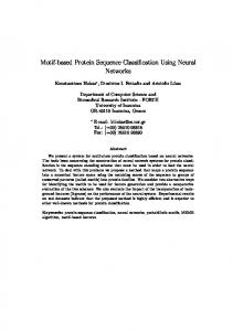
due to the large number of dimensions. Hence, using dimensionality reduction techniques can be crucial for the performance and the complexity of the learning algorithms. Models such as Principal Component Analysis [2], Latent Dirichlet Allocation [3] and Probabilistic Latent Semantic Analysis [4] are widely used to perform dimensionality reduction. Unfortunately, for very high-dimensional data, with hundreds of thousands of dimensions (e.g., 160, 000 4-grams), processing data instances into feature vectors at run time, using these models, is computationally expensive, e.g., due to inference at runtime in the case of LDA. A less expensive approach to dimensionality reduction is feature selection [5], [6], which reduces the number of features by selecting a subset of the available features based on some chosen criteria. In particular, feature selection by average mutual information [7] selects the top features that have the highest average mutual information with the class. The main disadvantages of feature selection are: (i) feature selection requires storing in memory the vocabularies of kgrams, which can become difficult given today’s very large collections of protein sequences, resulted due to progress on sequencing technologies [8]; and (ii) it does not allow for learning online features. Recently, a new approach to dimensionality reduction, called feature hashing has been introduced for text classification [9], [10], [11], [12], which offers a very inexpensive, yet effective, approach to reducing the number of features provided as input to a learning algorithm, and overcomes the disadvantages of feature selection. Feature hashing allows random collisions into the latent factors. Specifically, the original high-dimensional space is “reduced” by hashing the features, using a hash function, into a lower-dimensional space, i.e., mapping features to hash keys, where multiple features can be mapped (at random) to the same hash key, and “aggregating” their counts. Figure 1 shows the application of feature hashing on sparse high-dimensional feature spaces. Although very effective for reducing the number of features from very high dimensions (e.g., 222 ) to mid-size dimensions (e.g., 216 ), feature hashing can result in significant loss of information, especially when hash collisions occur between highly frequent features, with significantly different class distributions. In this paper, we study the applicability of feature hashing

xh

x

MALLQSRLLLSA RRAAATARASSW SHVEMGPPDPILG ···

protein sequence

M A L ··· MA AL ··· MAL ···

560 82 0 ··· feature 3575 hashing 34 ··· 34 ···

variable length k-grams

hashed features

w T xh

classification

Figure 1: Feature hashing on sparse high-dimensional feature spaces. Hashing is performed to reduce very high dimensions to mid-size dimensions, which does not significantly distort the data.

to protein sequence classification and address three main questions: (i) What is the influence of the hash size on the performance of protein sequence classifiers that use hash features, and what is the hash size at which the performance starts degrading, due to hash collisions? (ii) How effective is feature hashing on prohibitively high dimensional k-gram representations? (iii) How does the performance of feature hashing compare to that of feature selection by average mutual information? The results of our experiments on the three protein subcellular localization data sets show that feature hashing is an effective approach to reducing dimensionality on protein sequence classification tasks. The paper is organized as follows. In Section 2, we discuss the related work. We then provide background on feature selection and feature hashing in Section 3. Section 4 presents experiments and results, and Section 5 concludes the paper. II. R ELATED W ORK Feature Selection. Feature selection [5], [13], [7], is a dimensionality reduction technique, which attempts to remove redundant or irrelevant features in order to improve classification performance of learning algorithms. Feature selection methods have been widely used in Bioinformatics for tasks such as sequence analysis, e.g., prediction of protein function from sequence, gene prediction, where the features could be the amino acids or k-grams; microarray analysis; mass spectra analysis; and single nucleotide polymorphisms (SNPs) analysis, among others (see [14] for a review and the citations therein). Topic models. Topic models, such as Latent Dirichlet Allocation (LDA) [3], Probabilistic Latent Semantic Analysis (PLSA) [4], and Latent Semantic Indexing (LSI) [15] are dimensionality reduction models, designed to uncover hidden topics, i.e., clusters of semantically related words that co-occur in the documents. LSI uses singular value decomposition to identify topics, which are then used to represent documents in a low dimensional “topic” space. LDA models each document as a mixture of topics (drawn

from a conjugate Dirichlet prior), and each topic as a distribution over the words in the vocabulary. LDA has recently emerged as an important tool for modeling protein data. For example, Airoldi et al. [16] proposed the mixed membership stochastic block models to learn hidden protein interaction patterns. Pan et al. [17] used LDA to discover latent topic features, which correspond to hidden structures in the protein data, and input these features to random forest classifiers to predict protein interactions. However, topic models are computationally expensive, for example, LDA requires inference at runtime to estimate the topic distribution. Feature Abstraction. Feature abstraction methods [18], [19] are data organization techniques, designed to reduce a model input size by grouping “similar” features into clusters of features. Specifically, it learns an abstraction hierarchy over the set of features using hierarchical agglomerative clustering, based on the Jensen-Shannon divergence. A cut through the resulting abstraction hierarchy specifies a compressed model, where the nodes (or abstractions) on the cut are used as “features” in the classification model. Baker and McCallum [18] applied feature abstraction to reduce the dimensionality of the feature space for document classification tasks. Silvescu et al. [19] used it to simplify the data representation provided to a learner on biological sequence classification tasks. Feature Hashing. Shi et al. [9] and Weinberger et al. [10] presented hash kernels to map the high dimensional input spaces into lower dimensional spaces for large scale classification and large scale multitask learning (i.e., personalized spam filtering for hundreds of thousands of users), respectively. Ganchev and Dredze [20] empirically showed that hash features can produce accurate results on various NLP applications. Forman and Kirshenbaum [11] proposed a fast feature extraction approach by combining parsing and hashing for text classification and indexing. Hashing techniques have been also used in Bioinformatics. For example, Wesselink et al. [21] applied hashing to find the shortest contiguous subsequence that uniquely iden-

tifies a DNA sequence from a collection of DNA sequences. Buhler and Tompa [22] applied Locality-Sensitive Hashing (LSH) [23], a random hashing/projection technique, to discover transcriptional regulatory motifs in eukaryotes and ribosome binding sites in prokaryotes. Furthermore, Buhler [24] applied LSH to find short ungapped local alignments on a genome-wide scale. Shi et al. [9] used hashing to compare all subgraph pairs on biological graphs. In contrast to the approaches above, we used feature hashing, a very inexpensive approach, to reduce dimensionality on protein sequence classification tasks, and compared it with feature selection by average mutual information. Markov models. In the context of protein sequence classification, it is worth mentioning the fixed and variableorder Markov models (MMs), which capture dependencies between neighboring sequence elements. MMs are among the most widely used generative models of sequence data [25]. In a k th order MM, the sequence elements satisfy the Markov property: each element is independent of the rest given the k preceding elements. One main disadvantages of MMs in practice is that the number of parameters increases exponentially with the range k of direct dependencies, thereby increasing the risk of overfitting. Begleiter et al. [26] (and papers cited therein) have examined methods for prediction using variable order MMs, including probabilistic suffix trees, which can be viewed as variants of abstraction wherein the abstractions are constrained to share suffixes. III. M ETHODS The traditional k-gram approaches construct a vocabulary of size d, which contains all k-grams in a protein data set. A protein sequence is represented as a vector x with as many entries as the number of k-grams in the vocabulary. For a protein sequence, an entry i in x can record the frequency of k-gram i in the sequence, denoted by xi . Because only a small number of k-grams (compared to the vocabulary size) occur in a particular sequence, the representation of x is very sparse, i.e., only a small number of entries of x are non-zero. However, storing the parameter vectors in the original input space requires O(d) numbers, which can become difficult given today’s very large collections of protein and DNA sequence data. Feature selection reduces the size of the parameter vectors by selecting a subset of features from the original features, but still requires a mapping from strings to integers. Feature hashing eliminates the need for such a requirement by implicitly encoding the mapping into a hash function. Next, we briefly overview feature selection and feature hashing.

Algorithm 1 Feature Hashing Input: Protein sequence x; hash functions h and ξ, h : S → {0, · · · , b − 1}, ξ : S → {±1}. Output: Hashed feature vector xh . xh := [0, · · · , 0]; for all k-gram ∈ x do i = h(k-gram) % b; // Places k-grams into hash bins, from 0 to b-1. xhi = xhi + ξ(k-gram); // Updates the ith hash feature value. end for return xh // Records values of hash features.

ranked according to a scoring function and the top m best ranked features are selected. As the scoring function, we used the average mutual information [27] between the class variable Y and the random variable over the absence or presence of a feature xi in a document, denoted by Xi , which takes values 0 or 1, respectively. The average mutual information is defined as follows: I(Y, Xi )

= =

H(Y ) − H(Y |Xi ) (1) X X p(Y, Xi ) p(Y, Xi ) log p(Y )p(Xi ) Y ∈{yl } Xi ∈{0,1}

where H(Y ) is the entropy of the class variable, and H(Y |Xi ) is the entropy of the class variable conditioned on the absence or presence of feature xi . The probability p(Y, Xi ) is estimated from counts gathered from D, and p(Y ) and p(Xi ) are obtained by marginalizing p(Y, Xi ). The feature selection representation. Let (x, y) be an instance in D. The “bag of k-grams” representation of (x, y) is given by: (#x1 , · · · , #xd , yl ), where #xi , i = 1, · · · , d, represents the frequency counts of the k-gram xi in the protein sequence x. Given the selected set of features F = {xi1 , · · · , xib }, the instance (x, y) is transformed into (#xi1 , · · · , #xib , y) (see Figure 2a). B. Feature Hashing

A. Feature Selection by Average Mutual Information

Feature hashing [9], [10], [11], [12] is a dimensionality reduction technique, in which high-dimensional input vectors x of size d are hashed into lower-dimensional feature vectors xh of size b. The procedure for hashing a protein sequence x is shown in Algorithm 1 (see also Figure 1). Let S denote the set of all possible strings (or k-grams) and h and ξ be two hash functions, such that h : S → {0, · · · , b − 1} and ξ : S → {±1}, respectively. For a protein sequence x, each k-gram in x is directly mapped, using h1 , into a hash key, which represents the index of the k-gram in the feature vector xh , such that the hash key is a number between 0 and b − 1. Each index in xh stores the value

Feature selection can be used to perform dimensionality reduction by selecting a subset F of features from the set of k-grams (of size d) such that |F| = b. The features are

1 Note that h can be any hash function, e.g. hashCode() of the Java String class, or murmurHash function available online at http://sites.google.com/site/murmurhash/.

(“frequency counts”) of the corresponding hash feature. The hash function ξ indicates whether to increment or decrement the hash dimension of the k-gram, which renders the hash feature vector xh to be unbiased (see [10] for more details). Thus, an entry i in xh records the “frequency counts” of k-grams that are hashed together into the same hash key i. That is, X xhi = ξ(k)xk , (2) k:h(k)=i

for k = 0, · · · , d − 1 and i = 0, · · · , b − 1. Note that in the trivial case of ξ ≡ 1, xhi represents the actual frequency counts (see Figure 2b). As can be seen, multiple k-grams can be mapped, through h, into the same hash √ key. According to Birthday Paradox, if there are at least b features, then collisions are likely to happen [9], and hence, useful information for high accuracy classification could be lost through feature hashing. The kgrams in a collection of protein sequences typically follow a Zipf distribution, i.e., only very few k-grams occur with high frequency, whereas the majority of them occur very rarely (see Figure 3). Because hash collisions are independent of k-gram frequencies, most collisions are likely to happen between infrequent k-grams. Weinberger et al. [10] have proven that, for a feature vector x such that kxk2 = 1, the length of x is preserved with high probability, for sufficiently large dimension (or hash size) b and sufficiently small magnitude of x, i.e., kxk∞ (lower and upper bounds are theoretically derived). However, for many practical applications, the value of b can be smaller than the theoretical lower bound. This may be problematic as the smaller the size of the hash vector xh becomes, the more collisions occur in the data. Even a single collision of very high frequency words with different class distributions, can result in significant loss of information. IV. E XPERIMENTS AND R ESULTS In this section, we empirically study the applicability of feature hashing on three protein subcellular localization data sets: psortNeg2 introduced in [28], plant, and non-plant3 introduced in [29]. The psortNeg data set is extracted from PSORTdb v.2.0 Gram-negative sequences, which contains experimentally verified localization sites. Our data set consists of all proteins that belong to exactly one of the following five classes: cytoplasm (278), cytoplasmic membrane (309), periplasm (276), outer membrane (391) and extracellular (190). The total number of examples (proteins) in this data set is 1444. The plant data set contains 940 examples belonging to one of the following four classes: chloroplast (141), mitochondrial (368), secretory pathway/signal peptide (269) 2 www.psort.org/dataset/datasetv2.html 3 www.cbs.dtu.dk/services/TargetP/datasets/datasets.php

and other (consisting of 54 examples with label nuclear and 108 examples with label cytosolic). The non-plant data set contains 2738 examples, each in one of the following three classes: mitochondrial (361), secretory pathway/signal peptide (715) and other (consisting of 1224 examples labeled nuclear and 438 examples labeled cytosolic). A. Experimental Design Our experiments are designed to explore the following questions: (i) What is the influence of the hash size on the performance of biological sequence classifiers that use hash features, and what is the hash size at which the performance starts degrading, due to hash collisions? (ii) How effective is feature hashing on prohibitively high dimensional k-gram representations? (iii) How does the performance of feature hashing compare to that of feature selection by average mutual information? To answer these questions, we proceed with the following steps. We first preprocess the data by generating all the kgrams from each collection of sequences, i.e., generating all the contiguous (potentially overlapping) sub-sequences of length k, for various values of k. This is done by sliding a window of length k over sequences in each data set. Note that if a k-gram does not appear in the data, it is not considered as a feature4 . Given a protein sequence x, we apply feature hashing in two settings as follows: (i) We first generate all the k-grams of a fixed length k, i.e., k = 3. Each such k-gram is then hashed into a hash key. We refer to this setting as the fixedlength k-grams; (ii) We then generate all the k-grams of various lengths k, for values of k = 1, 2, 3, and 4. Thus, this setting uses the union of k-grams, for values of k from 1 to 4. Each such k-gram, i.e., unigram, 2-gram, 3-gram, or 4-gram, is hashed into a hash key. We refer to this setting as the variable-length k-grams. We train Support Vector Machine (SVM) classifiers [30] on hash features, in both settings, fixed-length and variablelength k-grams, and investigate the influence of the hash size on the performance of the classifiers. Specifically, we train SVM classifiers for values of the hash size ranging from a 1 bit hash to a 22 bit hash, in steps of 1, and compare their performance. Furthermore, we apply feature hashing to the sparse high dimensional variable-length k-gram representations to reduce the dimensionality to a mid-size b-dimensional space, e.g., b = 216 or b = 214 , and compare the performance of SVM classifiers trained using hashed features with that of their corresponding counterparts trained using feature selection. 4 The number of unique k-grams is exponential in k. However, for large values of k, many of the k-grams may not appear in the data (and, consequently, their frequency counts are zero). Note that the number of unique k-grams is bounded by the cardinality of the multiset of k-grams.

xs : x:

b−2 b−1

0

1

2

xs0

xs2

xs4

x0

x1

x2

x3

x4

0

1

2

3

4

···

xsd−3

xsd−1

xh :

···

xd−3 xd−2 xd−1

x:

d−3 d−2 d−1

b−2 b−1

0

1

2

xh 0

xh 1

xh 2

···

h xh b−2 xb−1

···

xd−3 xd−2 xd−1

x0

x1

x2

x3

x4

0

1

2

3

4

(a)

d−3 d−2 d−1

(b)

Figure 2: The transformation of “bag of k-grams” into: (a) feature selection, and (b) feature hashing representations.

6

4.5

5

4

4.5

5

4

3.5

3.5

log10 TF

log10 TF

3

log10 TF

4

2.5

3

2

2

1.5

2

4

6

8

10

variable length kïgrams

12

14

2

1.5

1

1

0.5

0.5

1

0 0

3

2.5

0 0

4

x 10

(a) non-plant

1

2

3

4

5

6

7

variable length kïgrams

8

0 0

4

x 10

(b) plant

2

4

6

8

variable length kïgrams

10 4

x 10

(c) psortNeg

Figure 3: The variable length k-grams in each protein data set: (a) non-plant, (b) plant, and (c) psortNeg, follow a Zipf distribution, i.e., only very few k-grams occur with high frequency, whereas the majority of them occur very rarely.

Specifically, the feature representations used in each case are the following: • a bag of b variable-length k-grams chosen from all d variable-length k-grams, using feature selection by average mutual information (See Section III.C for details). This experiment is denoted by FS. • a bag of b hash features obtained using feature hashing over all d variable-length k-grams, i.e., for each k-gram, feature hashing produces an index i such that i = h(kgram) % b. This experiment is denoted by FH. In our experiments, for SVM, we used the LibLinear implementation5 . As for the hash function, we experimented with both the hashCode of the Java String class, and murmurHash. We found that the results are not significantly different from one another in terms of the number of hash collisions and classification accuracy. We also experimented with both ξ : S → {±1} and ξ ≡ 1 - actual counts, and found that the results were not significantly different. The results shown in the next subsection use the hashCode function and ξ ≡ 1. On all data sets, we report the average classification accuracy obtained in a 5-fold cross validation experiment. The results are statistically significant (p < 0.05). The 5 Available

at http://www.csie.ntu.edu.tw/ cjlin/liblinear/

Bag of fixed or variable length k-grams 1-grams 2-grams 3-grams 4-grams (1-2)-grams (1-3)-grams (1-4)-grams (1-5)-grams

non-plant Accuracy % # features 71.21 20 70.85 400 79.80 7999 79.03 146598 70.56 420 79.69 8419 82.83 155017 80.09 950849

Table I: The performance of SVM classifiers trained using feature hashing on fixed length, 1-, 2-, 3-, 4-gram representations, as well as variable length, (1-2)-, (1-3)-, (1-4)-, (1-5)-grams representations, where the hash size is set to 222 , on the non-plant data set.

classification accuracy is shown as a function of the number of features. The x axis of all figures in the next subsection shows the number of features on a log2 scale (i.e., number of bits in the hash-table). B. Results Comparison of fixed length k-gram representations with variable length k-gram representations. Table I shows, on the non-plant data set, the performance of SVM classifiers trained using feature hashing on fixed length

80

88

82

78

86

Classification Accuracy

80

76

78

82

74

76

80

72

74

78

70

72

76

68

Baseline Feature Selection Feature Hashing

70 68 10

84

Classification Accuracy

Classification Accuracy

84

12

14

16

18

log2(Number of Features)

(a) non-plant

20

74

Baseline Feature Selection Feature Hashing

66 22

64 10

12

14

16

18

log2(Number of Features)

(b) plant

20

Baseline Feature Selection Feature Hashing

72 22

70 10

12

14

16

18

20

22

log2(Number of Features)

(c) psortNeg

Figure 4: Comparison of feature hashing with the “bag of variable length k-grams” approach, referred as baseline, and feature selection on the protein data sets: (a) non-plant, (b) plant, and (c) psortNeg, respectively, using (1-4)-grams representations.

as well as variable length k-gram representations, where the hash size is set to 222 . As seen in the table, the performance of SVMs trained on fixed length k-gram representations is worse than that of SVM classifiers trained using variable length k-gram representations, with (1-4)grams representation (i.e., k ranging from 1 to 4), resulting in the highest performance. This is expected as the protein sequence motifs, i.e., k-grams, have variable length. Hence, the performance of SVM classifiers trained using variable length k-gram representations increases as we add more dependencies in the data (i.e., larger values of k), but starts decreasing as k becomes greater than or equal to 5, due to overfitting. The number of variable length k-grams, for k ranging from 1 to 4, is 155, 017. Feature hashing eliminates the need for storing the vocabularies in memory by implicitly encoding the mapping from strings to integers into a hash function, and at the same time, allows for learning new online features. Similar results are obtained for the plant and psortNeg data sets (data not shown). We conclude that feature hashing is very effective on prohibitively high-dimensional n-gram representations, which would otherwise be impractical to use, resulting in memoryefficiency. Because (1-4)-grams representation results in the highest performance, we used it for subsequent experiments. The influence of hash sizes on classifiers’ performance. Figures 4a, 4b, and 4c show the influence of the hash size b on the performance of the SVM classifiers, trained using variable-length k-grams as feature representations, on the three protein data sets used in this study, non-plant, plant, and psortNeg, respectively. The values of b range from 210 to 222 . As can be seen in the figures, as the hash size b increases from 210 to 222 , the performance of SVM classifiers increases as well, due to a smaller rate of hash collisions

for larger values of b. Table II shows, on all three data sets used, the number of unique features and the percentage of collisions for various hash sizes. The number of unique features is calculated as the number of non-empty entries in the hash vector, and the number of collisions as the number of entries with at least one collision. Note that the percentage of collisions below 214 is 100%. As the hash size increases beyond 216 , the performance of SVM classifiers does not change substantially, and, eventually, converges. For example, on the non-plant data set, with 216 hash size, SVM achieves 81.3% accuracy, whereas with 222 hash size, SVM achieves an accuracy of 82.83% (Figure 4a). On the plant data set, SVMs achieve 78.4% and 78.51% accuracy, with 216 and 222 hash sizes, respectively (Figure 4b). Furthermore, as the hash size increases beyond 216 , the percentage of hash collisions decreases until no collisions occur (Table II). For all three data sets, with 222 hash size, there are no hash collisions. The performance of SVMs trained on hash features in the 222 dimensional space is matched by that of SVMs trained on hash features in the 218 dimensional space, suggesting that the hash collisions beyond 218 does not significantly distort the data. Because 222 (= 4, 194, 304) highly exceeds the number of unique features, and the rate of hash collisions becomes zero, this can be regarded as equivalent to the classifiers trained without hashing, which require storing the vocabularies in memory, referred as baseline (Figure 4). Moreover, we considered 216 as the point where the performance starts degrading. Note that the vocabulary sizes, i.e., the number of unique variable length k-grams, for non-plant, plant, and psortNeg, are 155, 017, 111, 544, and 124, 389, respectively. We conclude that, if feature hashing is used to reduce dimensionality from very large dimensions, e.g., 222 to mid-size dimensions, e.g., 216 , the hash collisions do not substantially hurt the classification accuracy, whereas if it is used to reduce dimensionality from mid-size dimensions to

Value of b 222 220 219 218 217 216 215 214

non-plant # features Collisions % 155017 0 153166 1.21 147223 5.29 132754 16.30 99764 45.04 59358 78.53 32474 95.80 16384 100

# features 111544 110236 107299 99913 82141 53616 31788 16384

plant Collisions % 0 1.18 3.95 11.43 31.38 64.29 89.56 100

psortNeg # features Collisions % 124389 0 122894 1.22 118871 4.64 109535 13.22 87618 35.66 55555 68.85 32075 92.02 16384 100

Table II: The number of unique features (denoted as # features) as well as the rate of collisions on non-plant, plant, and psortNeg data sets, respectively, for variable length k-gram representations, where k varies from 1 to 4.

smaller dimensions, e.g., 210 , the hash collision significantly distort the data, and the corresponding SVM classifiers result in poor performance. Comparison of feature hashing with baseline and feature selection. Figures 4a, 4b, and 4c also show the results of the comparison of feature hashing (FH) with baseline, i.e., the “bag of k-grams”, and feature selection (FS) on the three protein data sets, non-plant, plant, and psortNeg, respectively, for (1-4)-grams representations. As can be seen in the figures, feature hashing makes it possible to train SVM classifiers that use substantially smaller number of dimensions compared to the baseline, for a small or no drop in accuracy, for hash sizes between 216 and 222 . Furthermore, the performance of SVM classifiers trained using feature hashing is similar or slightly better compared to that of SVMs trained using feature selection, for hash sizes greater than 216 . For example, for 218 on nonplant, the SVM trained using feature hashing achieves an accuracy of 82.83%, whereas the SVM trained using feature selection, for the same hash size, achieves an accuracy of 81.37%. This can be due to removal of important sequence patterns, i.e., motifs, during the selection process. As the hash size decreases below 216 (and the hash collisions significantly distort the data), feature selection significantly outperforms feature hashing, for the same choice of the hash size. For example, for 214 , on non-plant, the SVMs trained using feature hashing and feature selection achieve an accuracy of 78.67% and 80.13%, respectively. However, for different choices of the hash size, the performance of feature selection is smaller than that of feature hashing, e.g., on the non-plant data set, with 214 , the accuracy of feature selection is 80.13%, whereas on the same data set, with 218 , the accuracy of feature hashing is 82.83%. We conclude that feature hashing results in slightly more accurate models compared to feature selection, for relatively large hash sizes. As the hash size decreases, feature selection significantly outperforms feature hashing, for the same choice of the hash size. However, similar to the baseline, feature selection requires storing the vocabularies in memory, and does not allow for learning new, online features.

V. C ONCLUSION We presented an application of feature hashing to reduce dimensionality of very high-dimensional feature vectors to mid-size feature vectors on protein sequence data. We compared feature hashing with feature selection, which is another dimensionality reduction technique. The results of our experiments on three protein subcellular localization data sets show that feature hashing is an effective approach to dealing with prohibitively highdimensional variable length k-gram representations. Feature hashing makes it possible to train SVM classifiers that use substantially smaller number of features compared to the approach which requires storing the vocabularies in memory, i.e., the “bag of k-grams” approach, while resulting in a small or no decrease in classification performance. Moreover, feature hashing results in slightly more accurate models compared to feature selection, for relatively large hash sizes. As the hash size decreases, feature selection significantly outperforms feature hashing. However, feature hashing has two main advantages over the “bag of k-grams” approach and feature selections, which are as follows: (i) does not require storing the vocabularies in memory, and (ii) allows for learning new, online features at runtime. Because recent advances in sequencing technologies have resulted in an exponential increase in the rate at which DNA and protein sequence data are being acquired [8], the application of feature hashing on biological sequence data advances the current state of the art in terms of algorithms that can efficiently process high-dimensional data into lowdimensional feature vectors at runtime. In the future, it would be interesting to investigate how the performance of hash kernels compares to that of histogrambased motif kernels for protein sequences, introduced by Ong and Zien [31], and the mismatch string kernels for SVM protein classification introduced by Lesli et al. [32]. Along the lines of dimensionality reduction, it would be interesting to compare the performance of feature hashing with that of feature abstraction [19] on protein sequence classification tasks. Furthermore, another direction is to apply feature hashing to other types of biological sequence data, e.g., DNA data, and other tasks, e.g., protein function prediction.

R EFERENCES [1] P. Baldi and S. Brunak, Bioinformatics: the Machine Learning Approach. MIT Press, 2001.

[18] D. Baker and A. McCallum, “Distributional clustering of words for text classification.” in Proc. of SIGIR-98, 1998.

Springer-

[19] A. Silvescu, C. Caragea, and V. Honavar, “Combining superstructuring and abstraction on sequence classification,” in ICDM, 2009, pp. 986–991.

[3] D. Blei, A. Ng, and M. Jordan, “Latent Dirichlet allocation,” Journal of Machine Learning Research, vol. 3, pp. 993–1022, 2003.

[20] K. Ganchev and M. Dredze, “Small statistical models by random feature mixing,” in Proceedings of the ACL-2008 Workshop on Mobile Language Processing. Association for Computational Linguistics, 2008.

[2] I. T. Jolliffe., Principal Component Analysis. Verlag, New York, 1986.

[4] T. Hofmann, “Probabilistic latent semantic analysis,” in Proc. of UAI’99, Stockholm, 1999. [5] I. Guyon and A. Elisseeff, “An introduction to variable and feature selection,” J. Mach. Learn. Res., vol. 3, pp. 1157– 1182, 2003. [6] F. Fleuret, “Fast binary feature selection with conditional mutual information,” J. Mach. Learn. Res., vol. 5, pp. 1531– 1555, 2004. [7] Y. Yang and J. O. Pederson, “Feature selection in statistical learning of text categorization.” in In Proceedings of ICML, 1997, pp. 412–420. [8] W. Ansorge, “Next-generation DNA sequencing techniques,” New Biotechnology, vol. 25, no. 4, pp. 195–203, 2009. [9] Q. Shi, J. Petterson, G. Dror, J. Langford, A. Smola, and S. Vishwanathan, “Hash kernels for structured data,” J. Mach. Learn. Res., vol. 10, pp. 2615–2637, 2009. [10] K. Weinberger, A. Dasgupta, J. Attenberg, J. Langford, and A. Smola, “Feature hashing for large scale multitask learning,” in Proc. of ICML, 2009. [11] G. Forman and E. Kirshenbaum, “Extremely fast text feature extraction for classification and indexing,” in Proc. of the 17th ACM CIKM, New York, NY, USA, 2008, pp. 1221–1230. [12] J. Langford, L. Li, and A. Strehl, “Vowpal wabbit online learning project.” 2007. [13] K. Kira and L. A. Rendell, “The feature selection problem: Traditional methods and a new algorithm.” in Proc. of AAAI, San Jose, CA, 1992, pp. 122–134. [14] Y. Saeys, I. n. Inza, and P. Larra˜naga, “A review of feature selection techniques in bioinformatics,” Bioinformatics, vol. 23, pp. 2507–2517, 2007. [15] S. Deerwester, S. T. Dumais, G. W. Furnas, T. K. Landauer, and R. Harshman, “Indexing by latent semantic analysis,” Journal of the American Society for Information Science, vol. 41, no. 6, pp. 391–407, 1990. [16] E. Airoldi, D. Blei, S. Fienberg, and E. Xing, “Mixed membership stochastic block models for relational data with application to protein-protein interactions,” in In Proc. of the Intl. Biometrics Society-ENAR Annual Meeting, 2006. [17] X.-Y. Pan, Y.-N. Zhang, and H.-B. Shen, “Large-scale prediction of human proteinprotein interactions from amino acid sequence based on latent topic features,” Journal of Proteome Research, vol. 9, no. 10, pp. 4992–5001, 2010.

[21] J.-J. Wesselink, B. delaIglesia, S. A. James, J. L. Dicks, I. N. Roberts, and V. Rayward-Smith, “Determining a unique defining dna sequence for yeast species using hashing techniques.” Bioinformatics, vol. 18, no. 2, pp. 1004–10, 2002. [22] J. Buhler and M. Tompa, “Finding motifs using random projections,” in Proceedings of the fifth annual international conference on Computational biology, ser. RECOMB ’01, 2001, pp. 69–76. [23] P. Indyk and R. Motwani, “Approximate nearest neighbors: towards removing the curse of dimensionality,” in Proceedings of the thirtieth annual ACM symposium on Theory of computing, ser. STOC ’98, 1998, pp. 604–613. [24] J. Buhler, “Efficient large-scale sequence comparison by locality-sensitive hashing,” Bioinformatics, vol. 17, no. 5, pp. 419–428, 2001. [25] R. Durbin, S. R. Eddy, A. Krogh, and G. Mitchison, Biological sequence analysis: Probabilistic Models of Proteins and Nucleic Acids. Cambridge University Press., 2004. [26] R. Begleiter, R. El-Yaniv, and G. Yona, “On prediction using variable order markov models,” Journal of Artificial Intelligence Res., vol. 22, pp. 385–421, 2004. [27] T. M. Cover and J. A. Thomas, Elements of Information Theory. John Wiley, 1991. [28] J. L. Gardy, C. Spencer, K. Wang, M. Ester, G. E. Tusnady, I. Simon, S. Hua, K. deFays, C. Lambert, K. Nakai, and F. S. Brinkman, “Psort-b: improving protein subcellular localization prediction for gram-negative bacteria,” Nucleic Acids Research, vol. 31, no. 13, pp. 3613–17, 2003. [29] O. Emanuelsson, H. Nielsen, S. Brunak, and G. von Heijne, “Predicting subcellular localization of proteins based on their n-terminal amino acid sequence.” J. Mol. Biol., vol. 300, pp. 1005–1016, 2000. [30] R.-E. Fan, K.-W. Chang, C.-J. Hsieh, X.-R. Wang, and C.-J. Lin, “LIBLINEAR: A library for large linear classification,” J. of Machine Learning Res., vol. 9, pp. 1871–1874, 2008. [31] C. S. Ong and A. Zien, “An automated combination of kernels for predicting protein subcellular localization.” in Proc. of WABI, 2008, pp. 186–179. [32] C. Leslie, E. Eskin, J. Weston, and W. S. Noble, “Mismatch string kernels for svm protein classification,” in Advances in Neural Information Processing Systems (NIPS 2002), 2002.