Efficient new-view synthesis using pairwise dictionary priors. O. J. Woodford. I. D. Reid. Department of Engineering Science,. University of Oxford.
Efficient new-view synthesis using pairwise dictionary priors O. J. Woodford I. D. Reid Department of Engineering Science, University of Oxford
A. W. Fitzgibbon Microsoft Research, Cambridge, U.K.
Abstract New-view synthesis (NVS) using texture priors (as opposed to surface-smoothness priors) can yield high quality results, but the standard formulation is in terms of largeclique Markov Random Fields (MRFs). Only local optimization methods such as iterated conditional modes, which are prone to fall into local minima close to the initial estimate, are practical for solving these problems. In this paper we replace the large-clique energies with pairwise potentials, by restricting the patch dictionary for each clique to image regions suitable for that clique. This enables for the first time the use of a global optimization method, such as tree-reweighted message passing, to solve the NVS problem with image-based priors. We employ a robust, truncated quadratic kernel to reject outliers caused by occlusions, specularities and moving objects, within our global optimization. Because the MRF optimization is thus fast, computing the unary potentials becomes the new performance bottleneck. An additional contribution of this paper is a novel, fast method for enumerating color modes of the per-pixel unary potentials, despite the non-convex nature of our robust kernel. We compare the results of our technique with other rendering methods, and discuss the relative merits and flaws of regularizing color, and of local versus global dictionaries.
1. Introduction The new-view synthesis (NVS) problem is this: given a set of images I1 to In of a 3D scene, compute the image V which would be obtained by placing the camera at a given new viewpoint that is not in the original set. It is a poorly constrained inverse problem and therefore effective priors are important if a good solution is to be obtained. The priors considered in this paper will all be defined in terms of energy functions applied to overlapping windows, or patches, in V. The parameter which most strongly controls the tractability of these problems is the size of these patches (the order of the prior). Historically, there has been a tradeoff in the selection of priors: high order priors can model the complex structures of the natural world
(a)
(b)
(c)
(d)
Figure 1. New view synthesis. (a) A synthesized, maximumlikelihood view, showing a large region of error. (b) Best result with high-order cliques [6], which uses discriminative, 5 × 5 patches, but with obligatory local optimization. While the optimum solution to this problem may well fix the errors, the optimizer cannot reach it, given (a) as start position. (c) Using 2 × 1 cliques with a sequence-specific, global dictionary. While a strong optimum to this problem can be found, the regularizer is not discriminative enough to correct the error. (d) Using 2 × 1 cliques with a local dictionary. The regularizer provides powerful discrimination, while enabling the optimizer to find a strong minimum.
(hair, trees, etc.) but tend to result in very difficult inference problems [6, 14]; while tractable (low order) priors can model only simple scene classes such as piecewise smooth shapes [11, 10]. The contribution of this paper is to exploit the structure of the NVS problem to represent natural scenes using tractable priors. This is not to say that good results cannot currently be obtained for NVS, under appropriate conditions. In stereo reconstruction for example, the assumption of piecewise smooth scene geometry can be expressed in an energy minimization framework which encodes the constraint that the depths of neighboring pixels in the solution should be similar, so the prior is of order 2. Depending on the precise form of the prior, a global optimum (or strong local optimum) of the energy can be computed efficiently using powerful inference algorithms1 such as tree-reweighted message passing [10] and graph cuts [1, 11]. When the piecewise smoothness assumption is approximately valid for the scene, these solutions yield high-quality synthesized views. However, as can be seen in figure 5, these methods produce unrealistic, blocky artifacts when applied to natural scenes. 1 Throughout the paper we shall use the term “global optimizer” to refer to algorithms of this type, which, although not necessarily guaranteed to find global optima, find strong optima in practise
It is possible to encode natural-world priors using patch dictionaries, which give excellent results for tasks such as constrained texture synthesis [12], inpainting [5] and newview synthesis [6]. However, energy minimization under these priors does not allow the use of global optimizers, so techniques such as iterated conditional modes (ICM) or simulated annealing must be used, with the associated poor tolerance to local minima or high computational cost respectively. The computational burden can be reduced by improving patch lookup [13, 18], but this does not fix the convergence problem. Criminisi et al. [3] use much smaller, local patch dictionaries (by restricting patch search to be near epipolar lines), which allows real-time computation of the prior, but again rely on ICM to impose the prior. Roth and Black’s “fields of experts” framework [14] replaces dictionary lookup with a continuous, filter-based prior, so that ICM may be replaced by gradient descent. In all cases, however, the dependence on local optimization remains, as does the concomitant requirement that the initial estimate of the solution be close to a good optimum. Woodford et al. [19] showed that simulated annealing does little to improve matters—if ICM converges to a poor solution, this typically means that large coherent search steps must be made to reach another optimum, and simulated annealing has a vanishingly small likelihood of making those steps. As noted above, priors such as piecewise smoothness in depth can be defined as the sum of energies defined on 2pixel patches, which enables very efficient inference. Priors over intensity rather than depth images, however, do not admit such a compact definition. From studies of the statistics of natural scenes [9, 15] the distribution of 2-pixel intensity patches is known to be well modeled by a t-distribution. When converted to a prior, this ultimately means that the most correct possible second order prior for natural intensity images is simply piecewise constant color—a poor regularizer for textured natural scenes. This means that to model general natural scenes we must go to larger patch sizes and hence to intractable inference. In new-view synthesis, however, the prior need not model all natural scenes; rather it should bias the output view to look like the input sequence. Thus one might try to learn a second order prior just over the input images. Figure 2 shows that this restriction is still equivalent to imposing piecewise smoothness, and we shall see that it fails to give a sufficiently powerful prior. However, narrowing the training samples further, to small regions of the input sequence, does usefully regularize the problem. We compare the new local prior to previous approaches on some image sequences containing complex geometry, and show that it achieves better solutions in considerably less time than previous methods. The main contribution of this paper then is to show how patch priors on NVS can be reduced to pairwise priors,
which allows for global inference. We argue that this is the first such reduction: although patch-based methods have previously been expressed using pairwise energies [4, 7], this is only for special problems in which the patches overlap only in pairs. This is because the number of unary terms is smaller than the number of output pixels: in superresolution [7], the number of unary terms is equal to the number of low-resolution input pixels; in texture quilting [4] the unary terms exist only at the boundaries of the region to be painted. In the NVS problem, there must be one patch per output pixel, with dense overlap. Reducing the overlap would require using a larger patch size when computing photoconsistency, which would further require the assumption of piecewise smooth scene geometry. In overview, our algorithm has two main steps: 1. the continuous problem of determining color at every output pixel is converted to a discrete problem by computing a small number of modes of the photoconsistency likelihood at every pixel. 2. One of these modes is selected at every pixel in order to maximize a combination of photoconsistency with the prior term, which prefers that patches of the output image look like patches from the input sequence. These steps are discussed in §3 and §4, after which §5 describes experimental comparisons of the new method with the state of the art.
2. Notation The new view V is a set of pixel colors {V (i)}M i=1 , defined in some appropriate color space, say R3 . Pixels are indexed by integers, in raster-scan order. A neighborhood, or clique, is a set of indices. For example, for a W × H image, the 4-connected neighbors of a non-boundary pixel i are the set N = {i − W, i − 1, i + 1, i + W }. The set of neighboring colors may then be written V (N). A neighborhood system is a set of neighborhoods, {Nj }N j=1 where N is the total number of neighborhoods in the image. We shall use a variety of neighborhood systems: • The patch neighborhood is denoted Pj , which for concreteness we shall say is a set containing the indices of pixels in the 5 × 5 window centered at pixel j. Again V (Pj ) is the patch viewed as a 5 × 5 image. Ignoring boundary effects, N = M , i.e. the number of cliques is the number of pixels. • The 4-connected neighbor system is the set {C4j }2M j=1 , with two cliques per pixel, again ignoring boundary bookkeeping, which might comprise the “north” cliques {i, i − W } and the “east” cliques {i, i + 1}. • The 8-connected neighbor system is the set {C8j }4M j=1 , with four cliques per pixel which add to those of the 4connected system the “north-east” clique {i, i−W +1} and the “south-east” clique {i, i + W + 1}.
potential colors at each pixel (see §3.1). This set is computed offline, so the minimization, rather than being over V, is over a label image L, with the energies φ and ψ being redefined with appropriate bookkeeping.
3. Unary energy: photoconsistency We begin by defining the unary energy φ which measures photoconsistency at every pixel. We use the following photoconsistency term, from [6]: (a)
(b)
(c)
Figure 2. Pairwise color priors. (a) Part of an image from the “Edmontosaurus” sequence. (b) Pairwise, negative log histograms of all 2x1 patches [I(i), I(i + 1)] in the input sequence, where I is (top to bottom respectively) the red, green and blue channel of the input patches. The dominant diagonals show that the global prior derived from the image sequence is still non-specific, effectively imposing the piecewise smoothness constraint that I(i) ≈ I(i + 1). (c) Binary histograms for the red, green and blue channel of horizontal 2x1 patches in the local dictionary generated for the pixel highlighted in (a). We show that local pairwise priors are more specific, producing better results.
We shall also consider the depth map Z, where z(i) is the depth of the scene at pixel i. We cast the problem in the framework of energy minimization, so the goal is to find the X (either V or Z or both) which minimizes an energy function X X E(X |φ1..M , ψ1..N ) = φi [X(i)] + ψj [X(Nj )] i
|
j
{z
unary energy
}
|
{z
}
prior (or clique) energy
(1) where the functions φi and ψj can be computed as a function of the input data. In [6] for example, φi : R3 → R+ is a measure of photoconsistency, and ψj : R5×5×3 → R+ gives the squared distance of the patch X = V (Pj ) to the closest patch in a dictionary T of exemplar patches, ψ(X) = minT∈T kT − Xk2 . Note that in this case φ varies with i, while ψ is independent of j. As another example, piecewise smooth regularization of depth has a similar unary term, but the neighborhood system is 4-connected (Nj = C4j ), and the prior term takes the form ψ({z, z 0 }) = %(|z − z 0 |) where %(·) is a robust kernel, for example the truncated quadratic %(t) = min(t2 , 1). As discussed above, clique size is the parameter which has most effect on tractability of the minimization, but a second important factor is the discretization of V . Although the above energies are written in terms of continuous variables, V and z, efficient optimization under arbitrary priors is possible only for discrete variables. To directly discretize V space—about 107 values for 8-bit RGB images—would be impractical. Our approach is to maintain a small set of
Ephoto (V (i), z(i)) =
n X
ρ(kCi (k, z(i)) − V (i)k)
(2)
k=1
where Ci (k, z) is the color (bilinearly interpolated) of the pixel in image Ik corresponding to pixel i in V at depth z, where depth is measured in the coordinate system of image V. We assume that all camera projection matrices are known and that the reader is familiar with the projection of points between views [8]. The robust kernel ρ(·) will generally be the truncated quadratic model ρ(x) = min(x2 , τ 2 )
(3)
where τ is a tuning parameter of the algorithm. This model assumes that pixels are generated either using an inlier process, whereby the input image samples are normally distributed, noisy measurements of some true color, or an outlier process, which models all other samples. It is similar to the generative model based approach of Strecha et al. [16]. For pure new-view synthesis, we are interested only in the color at each pixel, in which case Ephoto is a function only of V (i). Conversely, when doing multi-view reconstruction of depth, it is a function only of z. Therefore we define two “overloads” of Ephoto for these cases: Ephoto (V (i))
=
Ephoto (z(i))
=
min
zmin