theory formulates motion perception at two levels of inference: we first perform ... However, the integration strategy modeled by the slow-and-smooth prior may.
Motion integration using competitive priors Shuang Wu1 , Hongjing Lu2 , Alan Lee2 , and Alan Yuille1 1 2
Department of Statistics, UCLA Department of Psychology, UCLA
Abstract. Psychophysical experiments show that humans are better at perceiving rotation and expansion than translation [4][8]. These findings are inconsistent with standard models of motion integration which predict best performance for translation. To explain this discrepancy, our theory formulates motion perception at two levels of inference: we first perform model selection between the competing models (e.g. translation, rotation, and expansion) and then estimate the velocity using the selected model. We define novel prior models for smooth rotation and expansion using techniques similar to those in the slow-and-smooth model [23] (e.g. Green functions of differential operators). The theory gives good agreement with the trends observed in four human experiments.
1
Introduction
As an observer moves through the environment, the retinal image changes over time to create multiple complex motion flows, including translational, circular and radial motion. Imagine that you are in a moving car and seeing a walker through a set of punch holes, as illustrated in figure (1). In each hole, the component of the line motion orthogonal to the lines orientation can be clearly perceived; however, the component of motion parallel to the lines orientation is not observable. This is often referred to as the aperture problem. The inherent ambiguity of motion signals requires the visual system to employ an efficient integration strategy to combine many local measurements in order to perceive global motion. In the example (figure (1)), the visual system needs to effectively integrate local signals to perceive multiple complex motion flows, including the movement of the walker and the moving background respectively. Human observers are able to process different motion patterns and infer ego motion and global structure of the world. Psychophysical experiments have identified a variety of phenomena, such as motion capture and motion cooperativity [16], which appear to be consequences of such integration. A number of computational Bayesian models have been proposed to explain these effects based on prior assumptions about motion. In particular, it has been shown that a slowand-smooth prior, and related models, can qualitatively account for a range of experimental results [23, 21, 22] and can quantitatively account for others [9, 17]. However, the integration strategy modeled by the slow-and-smooth prior may not generalize to more complex motion types, such as circular and radial motion, which are critically important for estimating ego motion. In this paper we
2
Shuang Wu, Hongjing Lu, Alan Lee, and Alan Yuille
are concerned with two questions. (1) What integration priors should be used for a particular motion input? (2) How can local motion measurements be combined with the proper priors to estimate motion flow? Within the framework of Bayesian inference, the answers to these two questions are respectively based on model selection and parameter estimation. In the field of motion perception, most work has focused on the second question, using parameter estimation to estimate motion flow. However, Stocker and Simoncelli [18] recently proposed a conditioned Bayesian model in which strong biases in precise motion direction estimates arise as a consequence of a preceding decision about a particular hypothesis (left vs. right motion).
Fig. 1. An illustration of observing a walker with a moving camera. Top panel, three example frames. Bottom panel, observing the scene through a set of punch holes
The goal of this paper is to provide a computational explanation for both of the above questions using Bayesian inference. To address the first question, we develop new prior models for smooth rotation and expansion motion. To address the second, we propose that the human visual system has available multiple models of motion integration appropriate for different motion patterns. The visual system decides the best integration strategy based upon the perceived motion information, and this choice in turn affects the estimation of motion flow. In this paper, we first present a computational theory in section (4) that includes three different integration strategies, all derived within the same framework. We test this theory in sections (5,6) by comparing its predictions with human performance in psychophysical experiments, in which subjects were asked
Motion integration using competitive priors
3
to detect global motion patterns or to discriminate motion direction in translation (left vs. right), rotation (clockwise vs. counter-clockwise), and radial motion (inward vs. outward). We employ three commonly used stimuli: random dot patterns, moving gratings and plaids (two superimposed gratings each with different orientations) to show that the model can be applied to a variety of inputs. We compare the predictions of the model predictions with human performance across four psychophysical experiment.
2
Background
There is an enormous literature on visual motion phenomena and there is only room to summarize the work most relevant to this paper. Our computational model relates most closely to work [23, 21, 9] that formulates motion perception as Bayesian inference with a prior probability biasing towards slow-and-smooth motion. But psychophysical [4, 10, 1, 8], physiological [19, 3] and fMRI data [11] suggests that humans are sensitive to a variety of motion patterns including translation, rotation, and expansion. In particular, Freeman et al [4] and Lee et al [8] demonstrated that human performance on discrimination tasks for translation, rotation, and expansion motion was inconsistent with the predictions of the slow-and-smooth theory (our simulations independently verify this result). Instead, we propose that human motion perception is performed at two levels of inference: (i) model selection, and (ii) estimating the velocity with the selected model. The concept of model selection has been described in the literature, see [7], but has only recently been applied to model motion phenomena [18]. Our new motion models for rotation and expansion are formulated very similarly to the original slow-and-smooth model [23] and similar mathematical analysis [2] is used to obtain the forms of the solutions in terms of Greens functions of the differential operators used in the priors. Smoothness priors for motion have a long history in computer vision beginning with the influential work of Horn and Schunk [6] and related work by Hildreth [5]. The slow-and-smooth prior on the velocity [23] was developed to explain psychophysical phenomena such as motion capture [13]. The nature of the psychophysics stimuli and the experimental phenomena meant that the first derivative regularizers used in [6][5] needed to be supplemented by zeroth order regularizers (i.e. slowness of the velocity) and second, and higher, order regularizers. Specifically, higher order regularizers were required to ensure that the theory was well-posed for the sparse stimuli (e.g. moving dots) used in typical psychophysical experiments. Moreover, zeroth order regularizers were needed to ensure that the interactions (e.g. motion capture) between different stimuli decreased with distance [24]. Justifications for the slowness and smoothness assumptions came from analyzes of the probability distribution of velocity flow in the image plane assuming isotropic distributions of velocity in space [20, 25] which showed that for most distributions of velocity in space the projection onto the image plane would induce velocity distributions which were peaked at zero velocity and zero velocity gradient. More recently, empirical studies by Roth and
4
Shuang Wu, Hongjing Lu, Alan Lee, and Alan Yuille
Black [15] on motion statistics yield similar results. We note that a limitation of the slow-and-smooth prior, for computer vision purposes, is that it is a quadratic regularizer and hence tends to smooth the velocity over motion discontinuities (although the limited range of interaction of the slow-and-smooth model means that this effect is more localized than for standard quadratic regularizers). Hence non-quadratic regularizers/priors are preferred for computer vision applications. The nature of the psychophysical stimuli in this paper, however, means that discontinuities can be ignored and so we can use quadratic regularizers and take advantage of their good computational properties. In order to relate theories like slow-and-smooth to psychophysics we have to understand the experimental design and model how human subjects address the specific experimental tasks. The experiments we describe in this paper use a standard experimental design which we describe for dot stimuli (a similar design is used for gratings and plaid stimuli). For these stimuli, some of the dots (the signal) move coherently, whereas other dots (the noise) move randomly. The experimental task is to measure some property of the coherent stimulus (e.g. does it move to the left or the right? does it rotate or contract?). The difficulty of performing this task depends on the proportion of signal dots to noise dots. The coherence threshold is defined to be the value of the ratio at which human subjects achieve 75 % accuracy for the task. Hence the psychophysicist can adjust the parameters of the stimuli (i.e. proportion of signal to noise) until this degree of accuracy is obtained. To evaluate the performance of a theory, we compute the analogous threshold for the theory and compare it to the threshold found by the experiments. An alternative criterion is to measure the minimum speed or contrast (e.g. brightness of the dots compared to the background) required to achieve a certain performance level (e.g. 75 % accuracy) at a visual task (e.g. is the motion to the right or the left?).
3
Overview of the Theory
We formulate motion perception as a problem of Bayesian inference with two stages followed by post-processing. We hypothesize that the human visual system has a set of models M for estimating the velocity. Firstly, we perform model selection to find the model that best explains the observed motion pattern. Secondly, we estimate motion properties using the selected model. The postprocessing models how human subjects use the estimated motion to perform psychophysical tasks. Formally a model M estimates the velocity field {v} defined at all positions {r} in the image from local velocity measurements {u} at discrete positions {r i , i = 1, . . . N }. The model is specified by a prior p({v}|M ) on the velocity field and a likelihood function p({u}|{v}) for the measurements. This specifies a full distribution p({v}, {u}, M ) = p({u}|{v})p({v}|M )P (M ), where P (M ) is the prior over the models (which is a uniform distribution).
Motion integration using competitive priors
5
The prior and likelihoods are expressed as Gibbs distributions: p({v}|M ) = exp(−E({v}|M )/T ), p({u}|{v}) = exp(−E({u}|{v})/T ),
(1) (2)
and are specified in sections (4.1,4.2) respectively. The first stage of the theory selects the model M ∗ that best explains the measurements {u}. It is chosen to maximize the posterior of the model evidence: P ({u}|M )P (M ) M ∗ = arg max P (M |{u}) = arg max M M P ({u}) Z where p({u}|M ) = p({u}|{v})p({v}|M )d{v}.
(3) (4)
The second stage of the theory estimates the velocity flow by using the selected model M ∗ . This yields: v ∗ = arg max p({v}|{u}, M ∗ )
(5)
p({u}|{v})p({v}|M ∗ ) . p({u}|M ∗ )
(6)
v
where p({v}|{u}, M ∗ ) =
The form of these priors P ({v}) are distributions over functions, see section (4.1), which means that this model evidence will be computed by techniques similar to those used for Gaussian Processes [14]. The post-processing estimates the properties of the motion flow required to perform the psychophysics tasks. In the psychophysics experiments in this paper, the human subjects must determine whether the motion is translation, expansion/contraction, or rotation and then estimate the appropriate motion properties: (i) direction of motion (if translation), (ii) direction of expansion/contraction (if expansion/contraction), or (iii) direction of rotation (if rotation). To address these tasks, we use the following post-processing strategy which we illustrate for the rotation stimuli. First we compute the two stages of the theory as described above. If the rotation model is selected, then we estimate the center of rotation (by least squares fit) and compute the direction of rotation (i.e. clockwise or counterclockwise) for the velocity field evaluated at each data point (i.e. dots), see Appendix (C) for details. We alter the parameters of the stimuli (i.e. the proportion of noise dots) until 75 % of the stimulus data points are estimated to have the correct direction of rotation (for each stimulus). Alternatively, we consider a set of stimuli, compute the velocity flow for each stimulus and estimate the centers of rotation, compute the histograms of the estimated rotated directions for the data points for all images, and determine the stimulus parameters so that 75 % of the histogram values are in the correct direction.
4
Model Formulation
This section specifies the priors for the different models, the likelihood functions, closed form solutions for the velocity flows, and analytic formulae for performing model selection. Some details of the derivations are described in Appendix (A).
6
4.1
Shuang Wu, Hongjing Lu, Alan Lee, and Alan Yuille
The Priors
We define three priors corresponding to the three different types of motion – translation, rotation, and expansion. For each motion type, we encourage slowness and spatial smoothness. The prior for translation is very similar to the slow-and-smooth prior [23] except we drop the higher-order derivative terms and introduce an extra parameter (to ensure that all three models have similar degrees of freedom). We define the priors by their energy functions E({v}|M ), see equation (1). We label the models by M ∈ {t, r, e}, where t, r, e denote translation, rotation, and expansion respectively. (We note that the prior for expansion will also account for contraction). We use the convention that v = (vx , vy ). 1. Slow-and-smooth-translation: Z E({v}|M = t) =
λ(|v|2 + µ|∇v|2 + η|∇2 v|2 )dr,
(7)
2. Slow-and-smooth-rotation: Z ∂vx 2 ∂vy 2 ∂vx ∂vy 2 E({v}|M = r) = λ{|v|2 +µ[( ) +( ) +( + ) ]+η|∇2 v|2 }dr, ∂x ∂y ∂y ∂x (8) 3. Slow-and-smooth-expansion: Z ∂vx 2 ∂vy 2 ∂vx ∂vy 2 E({v}|M = e) = λ{|v|2 +µ[( ) +( ) +( − ) ]+η|∇2 v|2 }dr, ∂y ∂x ∂x ∂y (9) These priors are motivated as follows. The |v|2 and |∇2 v|2 terms bias towards slowness and smoothness and are used in all three models. However, the priors differ in the use of first derivative terms. The translation prior prefers constant translation motion with v constant, since ∇v = 0 for this type of motion. The translation prior is similar to the first three terms of the slow-and-smooth energy function [23] but with a restriction on the set of parameters. Formally λ(|v|2 + P∞ σ2 σ4 σ 2m 2 2 2 m 2 m=0 m!2m |D v| dr (for appropriate parameter 2 |∇v| + 8 |∇ v| )dr ≈ λ values). Our computer simulations showed that the translation prior performs similar to the original slow-and-smooth prior. The first derivative terms in the slow-and-smooth-rotation prior is motivated by the ideal form of rigid rotation: vx = −ω(y − y0 ), vy = ω(x − x0 )
(10)
where (x0 , y0 ) are the (unknown) centers, ω is the (unknown) angular speed. This rigid rotation is preferred by the slow-and-smooth-rotation prior (at least, ∂vy ∂vy ∂vx x by its first derivative terms), since we have ∂v ∂y + ∂x = 0 and ∂x = ∂y = 0 (independent of (x0 , y0 ) and ω).
Motion integration using competitive priors
7
The first derivative terms in the slow-and-smooth-expansion prior is motivated by the ideal form of rigid expansion: vx = e(x − x0 ), vy = e(y − y0 )
(11)
where (x0 , y0 ) are the (unknown) centers, and e is the (unknown) expansion rate. Such a rigid expansion is preferred by the slow-and-smooth-expansion prior (first ∂vy ∂vy ∂vx x order terms), since we have ∂v ∂x − ∂y = 0, and ∂y = ∂x = 0 (again independent of (x0 , y0 ) and e). Note that we will use equations (10,11) in the post-processing stage where we estimate the centers (x0 , y0 ) and the rotation/expansion ω, e, see Appendix (C). 4.2
The Likelihood Functions
The likelihood function differs for the three classes of stimuli used in the psychophysics experiments that we considered: (i) For moving dots, as used in [4], the motion measurement is the local velocity u of each dot (assumed known since the motion is small and so correspondence between dots at different time frames is unambiguous); (ii) For a moving grating [12] [8], the local motion measurement is the velocity component in the direction orthogonal to the grating orientation; (iii) For a moving plaid (with two superimposed grating each with different orientation) [12] [8], the local motion measurement uses the velocity components of each grating (effectively this reduces to the moving dot case). For the dot stimuli, the energy term in the likelihood function, see equation (2), is set to be E({u|v}) =
N X
|v(r i ) − u(r i )|2
(12)
i=1
For the grating stimuli, see figure (5), the likelihood function uses the energy function N X ˆ (r i ) − |u(r i )||2 En ({u}|{v}) = |v(r i ) · u (13) i=1
ˆ (r i ) is the unit vector in the direction of u(r i ) (i.e. in the direction of where u local image gradient and hence perpendicular to the orientation of the bar). For the plaid stimuli, see figure (6), the likelihood function uses the energy function Ep ({u}|{v}) =
N X
(|v(r i ) · uˆ1 (r i ) − |u1 (r i )||2 + |v(r i ) · uˆ2 (r i ) − |u2 (r i )||2 ) (14)
i=1
where there are two sets of measurements {u1 } and {u2 }. This specifies the velocity in two different directions and hence can be reformulated in terms of model for the dots.
8
4.3
Shuang Wu, Hongjing Lu, Alan Lee, and Alan Yuille
MAP estimator of velocities
The MAP estimate of the velocities for each model is obtained by solving v ∗ = arg max p({v}|{u}, M ) = arg min{E({u}|{v}) + E({v}|M )} v
v
(15)
For the slow-and-smooth model [23], it was shown using regularization analysis [2] that this solution v ∗ can be expressed in terms of a linear combination of the Green function G of the differential operator which imposes the slow-andsmoothness constraint (the precise form of this constraint was chosen so that G was a Gaussian [24]). In this paper, we perform a similar analysis for the three types of models M ∈ {t, r, e} introduced in this paper and show that the solution v ∗ can also be expressed as a linear combination of Green functions GM where M indicates the model. The precise forms of these Green functions are determined by the differential operators associated with the slow-and-smoothness terms of the models and are derived in Appendix (A). The main difference with the Green functions described by Yuille and Grzywacz [23],[25] is that the models for expansion/contraction and rotation require two vector valued Green functions M M M M M M M GM 1 = (G1x , G1y ) and G2 = (G2x , G2y ) (with the constraint that G1x = G2y M M and G2x = G1y ). These vector-valued Green functions are required to perform the coupling between the different velocity component required for rotation and expansion, see figure (2). For the translation model there is no coupling required M and so GM 2x = G1y = 0.
Fig. 2. The vector-valued Green function G = (G1 , G2 ). Top panel, left-to-right: =t M =r =e GM , GM for the translation, rotation, and expansion models. Bottom panel: 1x , G1x 1x M =t =r =e left-to right: G2x , GM , GM for translation, rotation, and expansion models. Ob2x 2x M =t serve that the GM are similar for all models, G2x vanishes for the translation model 1x M =r M =e (i.e. no coupling between velocity components), and G2x and G2x both have two peaks which correspond to the two directions of rotation and expansion. Recall that M M M GM 1x = G2y and G2x = G1y .
Motion integration using competitive priors
9
Our analysis, see Appendix (A), shows that the estimated velocities for model M M can be expressed in terms of the Greens functions GM 1 , G2 of the model and coefficients {αi }, {βi }: v(r) =
N X
M [αi GM 1 (r − r i ) + βi G2 (r − r i )],
(16)
i=1
where the coefficients {αi }, {βi } are obtained by solving linear equations, derived in Appendix (A), which depend on the likelihood function and hence on the form of the stimuli (e.g. dot, grating, or plaid). For the dot stimuli, the {α}, {β} are obtained by solving the linear equations: N X M [αj GM 1 (r i − r j ) + βj G2 (r i − r j )] + αi e1 + βi e2 = u(ri ), i = 1, . . . N, (17) i=j
where e1 , e2 denote the (orthogonal) coordinate axes (i.e. the x and y axes). If we express the {α}, {β} as two N-dimensional vectors A and B (recall N is the number of dots), the {ux } and {uy } as vectors U = (Ux , Uy ), and define M M M M M to have components GM , g2y , g1y , g2x N × N matrices g1x 1x (r i − r j ), G2x (r i − M M r j ), G1y (r i − r j ), G2y (r i − r j ) respectively, then we can express these linear equations as: µ ¶ µ ¶ µ M M¶ g1x g2x Ux A (18) = [ M M + I] g1y g2y Uy B For the grating stimuli, the {α}, {β} satisfy similar linear equations: µ ¶ µ ¶ µ M M¶ g˜ g˜2x A Ux + I] = [ 1x M M g˜2y g˜1y B Uy
(19)
M ˜ M (r i −r j ) = [GM (r i −r j )·ˆ u(ri )]ˆ ux (ri ), is the matrix with components G where g˜1x 1 1x M M M and similarly for g˜1y , g˜2x and g˜2y . For the plaid stimuli, the {α}, {β} satisfy: µ ¶ µ ¶ µ ¶ µ M M¶ µ M M¶ g˜1x g˜2x g˜ g˜2x A U1x U2x + I) = + , (20) + ( 1x M M M M g˜2y u g˜1y g˜1y g˜2y u B U1y U2y 1
2
where U1 , U2 are the velocity components of the two gratings respectively. These equations (18,19,20) can all be solved by matrix inversion to determine the coefficients {α}, {β}. These solutions can be substituted into equation (16) to obtain the velocity field. 4.4
Model Selection
We re-express model evidence p({u}|M ) in terms of (A, B): Z p({u}|M ) = p({u}|A, B, M )p(A, B|M )dAdB,
(21)
10
Shuang Wu, Hongjing Lu, Alan Lee, and Alan Yuille
where p({u}|A, B, M ), p(A, B|M ) are obtained by substituting the form of the velocity estimate, equation (16), and then normalizing these distributions. This is similar to how analogous terms are calculated for Gaussian Processors [14]. It can also be considered a variant of the Laplace approximation. The analysis is given in Appendix (B) and shows that the model evidence can be computed analytically be exploiting properties of multi-dimensional Gaussians. The result can be expressed compactly by introducing new notation in the form of 2N ×2N matrices: µ M M¶ µ M M¶ g1x g2x g˜1x g˜2x M M g = g˜ = . M M M M g1y g2y g˜1y g˜2y For the dot stimuli this gives:
p({u}|M ) =
1 1 gM p exp[− (U T U − U T M U )] T g +I (πT )N det(g M + I)
(22)
Similarly, for the gratings stimuli we obtain: p det(g M ) 1 1 ˜ −1 g˜M U )] q p({u}|M ) = exp[− (U T U − U T g˜M Σ N (πT ) T ˜ det(Σ)
(23)
˜ = g˜M g˜M + g M . where Σ For the plaids stimuli we obtain: (we omit the M in g M to simplify notation.) p det(g) 1 1 ˜ −1 Φ] (24) q p({u1 }, {u2 }|M ) = exp − [U1T U1 + U2T U2 − ΦT Σ N (πT ) T ˜ det(Σ) ˜ = g˜M g˜M + g˜M g˜M + g M and Φ = g˜T U1 + g˜T U2 . where Σ 2 1 2 2 1 1
5
Experiment 1: random dot motion
We first investigate motion perception with the moving dots stimuli (figure 3) used by Freeman and Harris [4]. The stimuli consisted of 128 moving dots in a display window. All the dots in the stimulus had the same speed in all the three motion patterns, including translation, rotation and expansion. The reported simulations are based upon 1000 trials for each speed condition. The parameter values used in the simulations are λ = 0.001, µ = 12.5, η = 78.125 and T = 0.0054. Model selection results are shown in the panels of figure (4). It is shown that the correct model is always selected over the entire range of speed, and for all 3 type of motion stimuli.
Motion integration using competitive priors 2.5
2.5
2
2
1.5
1.5
1
1
0.5
0.5
0
0
−0.5
−0.5
−1
−1
−1.5
−1.5
−2
−2
−2.5 −3
−2.5 −3
−2
−1
0
1
2
3
4
11
3
2
1
0
−1
−2
−2
−1
0
1
2
−3 −3
3
−2
−1
0
1
2
3
Fig. 3. Moving random dot stimuli – translation, rotation and expansion 482.9
482
rotation model expansion model translation model
482
rotation model expansion model translation model
481
rotation model expansion model translation model
481
480
log(P(u))
log(P(u))
log(P(u))
482.85
479
480
479
482.8 478
482.75 0.05
0.06
0.07 0.08 speed
0.09
0.1
477 0.05
478
0.06
0.07 0.08 speed
0.09
0.1
477 0.05
0.06
0.07 0.08 speed
0.09
0.1
Fig. 4. Model selection results in Experiment 1 with random dot motion. Plots the log probability of the model as a function of speed for each type of stimuli. left: translation; middle: rotation; right: expansion. Green curves with cross are from translation model. Red curves with circles are from rotation model. Blue curves with squares are from expansion model.
6 6.1
Experiment 2: randomly oriented gratings Stimulus
When randomly oriented grating elements drift behind apertures, the perceived direction of motion is heavily biased by the orientation of the gratings, as well as by the shape and contrast of the apertures. Recently, Nishida and his colleagues developed a novel global motion stimulus consisting of a number of gratings elements, each with randomly assigned orientation [12]. Lee and his colleagues [8] extended this stimulus to rotational and radial motion. A coherent motion in this type of stimuli is perceived when the drifting velocities, also termed the component of velocity, of elements are consistent with a given global motion pattern. Examples of the stimuli used in these psychophysical experiments are shown in left side of figure (5). The stimuli consisted of 728 gratings (drifting sine-wave gratings windowed by stationary Gaussians). The orientations of the gratings were randomly assigned, and their drifting velocities were determined by a specified global motion. The motions of signal grating elements were consistent with global motion, but the motions of noise grating elements were randomized. The task was to identify the global motion direction as one of two alternatives: left/right for translation, clockwise/counterclockwise for rotation, and inward/outward for expansion. Motion sensitivity was measured by the coherence threshold, defined as the proportion of signal elements that yielded a performance level of 75% correct.
12
Shuang Wu, Hongjing Lu, Alan Lee, and Alan Yuille
Similar stimuli with 328 gratings were generated to test our computational models. The smaller grating number is used to shorten simulation time, and experiments show that model behavior remains the same when grating number increases. The input for the models is the component velocity perpendicular to the assigned orientation for each grating. Two levels of inference are involved. Our simulations first select the correct model for each stimulus and then estimate the velocity flow using the selected model. All reported simulations in Experiment 2-4 are based up 50 trials for each level of coherence ratio. The parameter values used in the simulations are µ = 12.5, η = 78.125, v = 0.0244 and T = 4 exp −5.0. For rotation/expansion model, λ = 0.005; for translation model, λ = 0.0025. 6.2
Model selection results
Model selection results are shown in tables (1,2,3). From the table we see that the rotation model has the highest model evidence for the rotation stimulus over the entire range of the coherence ratio. As coherence ratio increases, the advantage of rotation model over the other two models also increases. Analogous results are found for the expansion stimuli. However, for translation stimulus, all models have very similar model evidence values. This is caused by translation being favored by all three models, and indeed they all produce very similar motion field estimates. 6.3
Comparison between human performance and model prediction
Once the appropriate model has been selected, the velocity flow is estimated using the selected model (more specifically, this is computed from equations (16,17) with the appropriate M ). The post-processing in Experiments 2 4 includes a simple decision rule the input of which is the velocity flow estimated by the selected model.First the selected model estimates velocity flow in each trial. At each level of coherence ratio in the range of 0 to 50%, the post-processing enables the model to predict accuracy in discriminating motion direction for each stimulus (e.g., left vs. right for translation, clockwise vs. counter-clockwise for rotation, and inward vs. outward for expansion). To address this task, we pool estimated motion directions of 328 elements to generate a motion direction histogram for each trial. Note we use rotation direction and expansion direction to generate histograms. We then compute the average direction histogram over 50 trials for stimuli with one moving direction (e.g., P (v|L) for leftward translation), and the average direction histogram over 50 trials for stimuli with the opposite moving direction, P (v|R) for rightward translation. Based on the two computed histograms, a decision boundary is searched to achieve maximum accuracy. We apply the same postprocessing on each of the three motion patterns to estimate accuracy at each level of coherence ratio, and then estimate the coherence threshold needed to achieve 75% correct in the discrimination task.
Motion integration using competitive priors
coherence ratio rotation model expansion model translation model
10% 1009.0 1008.9 1008.9
20% 1060.1 1059.5 1059.7
30% 1146.3 1144.9 1145.5
40% 1256.9 1254.4 1255.5
13
50% 1418.8 1414.7 1416.5
Table 1. Model selection result for the grating rotation stimuli. The values are logarithms of model evidence. The correct model, rotation model, always wins. As the coherence ratio increases, the rotation model’s advantage also increases. coherence ratio rotation model expansion model translation model
10% 1011.5 1011.7 1011.6
20% 1057.4 1058.0 1057.6
30% 1151.8 1153.4 1152.5
40% 1275.9 1278.5 1277.1
50% 1430.0 1434.2 1431.9
Table 2. Model selection result for the grating expansion stimuli. The correct model, expansion, always wins. coherence ratio rotation model expansion model translation model
10% 990.2 990.2 990.2
20% 1076.3 1076.2 1076.2
30% 1159.7 1159.7 1159.7
40% 1265.6 1265.7 1265.6
50% 1456.1 1456.3 1456.2
Table 3. Model selection result for the grating translation stimuli. All three models (rotation/expansion/translation) have virtually the same model evidence. This is due to the fact that rotation/expansion models also favor translation as translation model does.
14
Shuang Wu, Hongjing Lu, Alan Lee, and Alan Yuille
The results of psychophysical experiments (middle panel of figure 5) showed worse performance for perceiving translation than rotation/expansion motion [8]. Clearly, as shown in the third panel of the same figure, the model performs best for rotation and expansion, and is worst for translation. This finding agrees with human performance in psychophysical experiments.
Human
Model 0.25 Coherence Ratio Threshold
Coherence Ratio Threshold
0.5 0.4 0.3 0.2 0.1 0
translation
rotation
expansion
0.2 0.15 0.1 0.05 0
translation
rotation
expansion
Fig. 5. Stimulus and results in Experiment 2 with randomly-oriented grating stimuli. Left panel: illustration of grating stimulus. Blue arrows indicate the drifting velocity of each grating. Middle panel: human coherence thresholds for different motion stimuli. Right panel: Model prediction of coherence thresholds which are consistent with human trends.
7 7.1
Experiment 3: plaid stimuli Stimulus
A plaid pattern consists of two drifting gratings arranged such that their individual orientations are orthogonal (see illustration in the left panel of figure 6). The drifting velocities of the two gratings in one plaid are determined by the global motion and their orientations. As the point of intersection for two superimposed gratings provides a tracking feature, the plaid stimulus reduces ambiguity in the measurement of local motion. The experimental methods were the same as those used in Experiment 2, except plaid elements were replaced by grating elements. 7.2
Results
As shown in the middle panel of figure 6, human observers exhibited the worst performance (highest thresholds) in discriminating motion directions in translation, as compared to rotation and radial motion. The right panel of figure 6 shows the model’s performance, which matches human performance quantitatively. Notably, the model predicts better performance for plaid stimuli (Exp 3) than for grating stimuli (Exp 2), which is consistent with human performance.
Motion integration using competitive priors Human
Model 0.25 Plaids Gratings
0.4 0.3 0.2 0.1
translation
rotation
expansion
Coherence Ratio Threshold
Coherence Ratio Threshold
0.5
0
15
Plaids Gratings 0.2 0.15 0.1 0.05 0
translation
rotation
expansion
Fig. 6. Stimulus and results in plaid experiment in Experiment 3 with plaid stimuli. Left panel: illustration of plaid stimulus. Blue arrows indicate the drifting velocity of each grating. Middle panel: human coherence thresholds for different motion stimuli. Right panel: Model prediction of coherence thresholds which are consistent with human trends.
8 8.1
Experiment 4: Results for non-rigid rotation and radial motion Stimulus
In each of the previous three experiments, all the elements were assigned the same speed, which yielded non-rigid rotation and radial motion. However, in a rigid motion pattern, the assigned speed for each element should vary according to the distance to the center of rotation and radial motion. In Experiment 4, we assessed whether rigidity could affect human motion performance in perceiving rotation and radial motion. We introduced a rigid rotation condition, in which element speeds were determined by a constant rotation velocity and the distance of the element to the rotation center. The average speed was kept the same as that used in non-rigid rotation condition. Similar manipulations were employed for the rigid radial-motion condition. The experimental methods were the same as those employed in Experiment 2 with the grating stimulus. 8.2
Results
As shown in figure 7 (left panel), human observers were not sensitive to rigid versus non-rigid rotation and radial motion (in the current experimental conditions). This result is consistent with previous findings reported in the literature [1]. The right panel in figure 7 shows the model’s predictions, which qualitatively match human performance across the four conditions. Although the rotation and expansion priors were motivated by rigid rotation and expansion, the results in Experiment 4 clearly the priors are ”robust” to non-rigid
9
Conclusion
We propose a computational theory for motion perception which proceeds in two stages. The first stage selects the best model to explain the data from a
16
Shuang Wu, Hongjing Lu, Alan Lee, and Alan Yuille Human
Model 0.2 Non−rigid Rigid
0.6 0.5 0.4 0.3 0.2 0.1 0
rotation
expansion
Coherence Ratio Threshold
Coherence Ratio Threshold
0.7
Non−rigid Rigid 0.15
0.1
0.05
0
rotation
expansion
Fig. 7. Results in Experiment 4 with grating stimuli to compare rigid versus nonrigid rotation and expansion. Left panel: human coherence thresholds for rigid and non-rigid conditions as a function of different motion patterns. Right panel: Model prediction of coherence thresholds which are consistent with human trends.
set of competing models. The second stage estimates the velocity field using the selected model. In this paper, we used three competing models for translation, rotation, and expansion. We defined novel priors for rotation and expansion by analogy to the slow-and-smooth prior proposed by Yuille and Grzywacz [23, 24] and showed that the velocity estimation could be expressed as a linear combination of Green functions. We showed that model selection correctly selects the appropriate model for several different stimulus conditions and that the selected model estimates a plausible velocity field. We compared our competitive prior theory to the performance of human subjects on threshold tasks using different types of stimuli. Our results on random dot stimuli were in general agreement with the experimental findings of Freeman and Harris [4]. We also found good agreement with the experimental findings of our group [8] for grating and plaid stimuli. But there are current limitations to our results since different parameter settings are required for the model estimation and the velocity estimation tasks. We are exploring two possibilities: (i) for the psychophysics stimuli the human subjects are aware that the centers of expansion and rotation are at the center of the image, but this information is not currently being used in our theory (but can be inserted as an additional requirement), (ii) humans may be better at observing expansion/rotation than translation since attention and eye movements (A. Glennerster – private communication) may be used to remove the translational components leaving only expansion/rotation, but this is not included in our model. Our current work aims to resolve these issues and extend these findings to a range of different motions (e.g. affine motion) and to use increasingly naturalistic appearance/intensity models. It is also important to determine if motion patterns to which humans are sensitive correspond to those appearing regularly in natural motion sequences. Acknowledgments We gratefully acknowledge funding from NSF 0736015 and 0613563. We thank Xuming He for feedback.
Motion integration using competitive priors
17
Appendix A This appendix gives the derivations of the formulae for estimating velocity. In particular, it justifies that the MAP estimate of the velocity is of form: v(r) =
N X
M [αi GM 1 (r − r i ) + βi G2 (r − r i )]
i=1
as stated in equation (16), and the {α}, {β} are given by equations (17) for the dot, grating, and plaid stimuli. This generalizes the derivation of the original slow-and-smooth model [23, 24]. We first re-express the prior in terms of a differential operator (A.1), show that the MAP estimate can be expressed in terms of Green functions of the differential operator (A.2), and then show how to solve for the Green functions (A.3). A.1 Re-express the Prior in terms of a Differential Operator D We use the quadratic form of the energy functions of the priors, see equations (7, 8, 9), to re-express them in terms of a differential operator DM indexed by the model M. Z E({v}|M ) = v · (DM v)dr. (25) This re-expression is performed by functional integration (assuming suitable boundary conditions as |r| 7→ ∞) and yields: µ ¶ Z Z 10 |v|2 dr = v T vdr 01 µ 2 ¶ Z Z ∇ 0 (|∇vx |2 + |∇vy |2 )dr = − v T vdr 0 ∇2 Ã ! Z Z Z ∂2 0 ∂vx ∂vy ∂vx ∂vy T ∂x∂y vdr = 2 dr = − v dr 2 ∂2 ∂y ∂x ∂x ∂y 0 ∂x∂y µ 2 2 ¶ Z Z (∇ ) 0 2 2 T |∇ v| dr = v vdr 0 (∇2 )2 Combining the terms for the different priors E(v|M ) gives the operators: µ 2 ¶ µ 2 2 ¶ ∇ 0 (∇ ) 0 Dt = λ(I − µ + η ) 0 ∇2 0 (∇2 )2 ! Ã µ 2 2 ¶ ∂2 ∇2 ∂x∂y (∇ ) 0 + η ) Dr = λ(I − µ 2 ∂ 2 0 (∇2 )2 ∂x∂y ∇ Ã ! µ 2 2 ¶ ∂2 ∇2 − ∂x∂y (∇ ) 0 De = λ(I − µ + η ) 2 0 (∇2 )2 − ∂ ∇2 ∂x∂y
18
Shuang Wu, Hongjing Lu, Alan Lee, and Alan Yuille
A.2 The Euler-Lagrange Equations The MAP estimate {v} for model M , {v ∗ } = arg max{v} P ({v}|{u}, M ), is obtained by solving the Euler-Lagrange equations for the functional E({u}|{v}) + E({v}|M ). This equation will depend on the form of the stimuli (e.g. dots and gratings). For the dot stimuli, we express the functional in the form: E({u}|{v}) + E({v}|M ) =
Z X N
Z |v(r) − u(r i )|2 δ(r − r i )dr +
v · (DM v)dr
i=1
(26)
This gives Euler-Lagrange equation: N X
2[v(r) − u(r i )]δ(r − r i ) + 2DM v(r) = 0.
(27)
i=1
The solution can be obtained (extending [2] and [24]) by assuming a solution M expressed as linear combination of vector valued Green’s functions GM 1 , G2 : v(r) =
N X
M [αi GM 1 (r − r i ) + βi G2 (r − r i )],
(28)
i=1 M where {α}, {β} are coefficients and GM 1 , G2 are the solutions of µ ¶ µ ¶ δ(0) 0 DM G1 (r) = = e1 , DM G2 (r) = = e2 0 δ(0)
The form of the priors, and hence the Green functions, ensures that this solution is well-posed at the data points and falls off smoothly as r 7→ ∞. More specifically: (i) the second order derivative terms in the priors ensure that G1 (0) and G2 (0) are finite [24], and (ii) the slowness term ensures that the Green functions decrease to zero as |r| 7→ ∞ [24]. We obtain the linear equations for {α}, {β}, given by equation (17), by substituting equation (28) into the Euler-Lagrange equations (27), using the Green functions from equation (9). For the grating stimulus, we obtain similar results. The energy functional becomes:
E({u}|{v})+E({v}|M ) =
Z X N
Z |v(r)·ˆ u(r i )−u(r i )|2 δ(r−r i )dr+
v·(DM v)dr.
i=1
(29)
This gives Euler-Lagrange equations: N X ˆ (r i )]ˆ {[v(r) · u u(r i ) − u(r i )}δ(r − r i ) + DM v(r) = 0. i=1
(30)
Motion integration using competitive priors
19
The solution v can be expressed in form given by equation (28) with the same Green functions from equation (9). Substituting the form of v into the Euler-Lagrange equation (30) gives the linear equation (19) for the {α}, {β}. A.3. Solving for the Green Functions We solve equation (9) for the Green functions by Fourier transforms. Denote G1 (r) = (G1x (r), G1y (r))T (we drop the model index M to simplify notation). This gives the following solutions for the three different cases: 1. Slow-and-smooth-translation: We apply Fourier transforms to the equation for the Green functions: ¶µ µ ¶ µ ¶ G1x 1 − µ∇2 + η(∇2 )2 0 δ(0) λ = 0 1 − µ∇2 + η(∇2 )2 G1y 0 to obtain linear equations for the Fourier transforms FG(ωx , ωy ) (where ω 2 = ωx2 + ωy2 ): ¶ µ ¶ µ ¶µ FG1x 1 1 + µω 2 + ηω 4 0 = λ FG1y 0 0 1 + µω 2 + ηω 4 which is solved to give µ
FG1x FG1y
1 = λ
µ
1 1+µω 2 +ηω 4
0
with similar solution for FG2 . 2. Slow-and-smooth-rotation: we re-express the Green function equation in fourier space à !µ ¶ µ ¶ ∂2 1 − µ∇2 + η(∇2 )2 −µ ∂x∂y G1x δ(0) λ = 2 G1y 0 −µ ∂ 1 − µ∇2 + η(∇2 )2 ∂x∂y
µ λ
1 + µω 2 + ηω 4 µωx ωy µωx ωy 1 + µω 2 + ηω 4
defining
µ dr = det[
¶µ
FG1x FG1y
¶ =
µ ¶ 1 0
¶ 1 + µω 2 + ηω 4 −µωx ωy ] −µωx ωy 1 + µω 2 + ηω 4
gives the solution µ ¶ µ ¶µ ¶ 1 FG1x 1 + µω 2 + ηω 4 −µωx ωy 1 = FG1y −µωx ωy 1 + µω 2 + ηω 4 0 λdr 3. Slow-and-smooth-expansion: this is a simple modification of the rotation case: !µ à ¶ µ ¶ ∂2 1 + µ∇2 + η(∇2 )2 −µ ∂x∂y FG1x 1 λ = ∂2 FG1y 0 −µ ∂x∂y 1 + µ∇2 + η(∇2 )2
20
Shuang Wu, Hongjing Lu, Alan Lee, and Alan Yuille
yields the solution µ ¶ µ ¶µ ¶ 1 FG1x 1 + µω 2 + ηω 4 µωx ωy 1 = FG1y µωx ωy 1 + µω 2 + ηω 4 0 λde Note that the following equalities hold for both rotation and expansion: G1x (x, y) = G2y (y, x), G1y (x, y) = G2x (x, y) B. Model Selection The model evidence is
Z
p({u}) =
p({u}|{v})p({v})d{v}
which we re-express in term of (A, B) Z p({u}) = p({u}|A, B)p(A, B)dAdB in which p({u}|A, B) =
1 1 exp(−E({u}|A, B)/T ), p(A, B) = exp(−E(A, B)/T ) Z1 Z2
where, for the random dot stimuli, E({u}|A, B) =
N X
|v(r i ) − u(r i )|2 = ΦT G2 Φ − 2U T GΦ + U T U,
(31)
i=1
where Φ = (AB)T . We can re-express this as: E(A, B) = ΦT GΦ, PN PN using v(r) = i=1 [αi G1 (r − r i ) + βi G2 (r − r i )] and Dv(r) = i=1 [αi δ(r − r i )e1 + βi δ(r − r i )e2 ]. The partition functions are of form: Z Z Z1 = exp(−E({u}|A, B)/T )d{u} = exp(−(U − V )T (U − V )/T )dU = (πT )N Z Z (πT )N Z2 = exp(−E(A, B)/T )dAdB = exp(−ΦT GΦ/T )dΦ = p det(G) We now re-express the model evidence p({u}), Z 1 1 p({u}) = exp(−E({u}|A, B)/T ) exp(−E(A, B)/T )dAdB Z1 Z2 Z 1 1 = exp[− (ΦT (G2 + G)Φ − 2U T GΦ + U T U )]dΦ Z1 Z2 T
Motion integration using competitive priors
21
denoting Σ = G2 + G = GH, H = G + I, Θ = Σ −1 GU = H −1 U gives Z 1 1 exp[− (ΦT ΣΦ − 2U T GΦ + U T U )]dΦ Z1 Z2 T Z 1 1 = exp[− ((Φ − Θ)T Σ(Φ − Θ) + U T U − ΘT ΣΘ)]dΦ Z1 Z2 T Z 1 1 1 T = exp[− (U U − ΘT ΣΘ)] exp{− [(Φ − Θ)T Σ(Φ − Θ)]}dΦ Z1 Z2 T T p det(G) 1 1 T (πT )N T p = exp[− (U U − Θ ΣΘ)] (πT )N (πT )N T det(Σ) 1 1 T p = exp[− (U U − U T H −1 U )]. T (πT )N det(G + I)
p({u}) =
Modification for the Grating Stimulus In the model selection stage we modify the energy to be,
E({u}|A, B) =
N X
ˆ (r i ) − u(r i )|2 |v(r i ) · u
i=1
˜ + UT U ˜ − 2U T GΦ ˜ T GΦ = ΦT G Z E(A, B) =
v · (Dv)dr = ΦT GΦ
The partition functions Z1 and Z2 remain the same. So Z
1 1 exp(−E({u}|A, B)/T ) exp(−E(A, B)/T )dAdB Z1 Z2 Z 1 1 ˜T G ˜ + G)Φ − 2U T GΦ ˜ + U T U )]dΦ = exp[− (ΦT (G Z1 Z2 T
p({u}) =
denoting ˜ =G ˜T G ˜ + G, Θ ˜=Σ ˜ −1 G ˜T U Σ
22
Shuang Wu, Hongjing Lu, Alan Lee, and Alan Yuille
˜ is symmetric even though G ˜ is not) we get: and (noting that Σ Z 1 1 ˜ − 2U T GΦ ˜ + U T U )]dΦ p({u}) = exp[− (ΦT ΣΦ Z1 Z2 T Z 1 1 ˜ T Σ(Φ ˜ − Θ) ˜ + UT U − Θ ˜T Σ ˜ Θ)]dΦ ˜ exp[− ((Φ − Θ) = Z1 Z2 T Z 1 1 1 ˜T Σ ˜ Θ)] ˜ ˜ T Σ(Φ ˜ − Θ)]}dΦ ˜ exp{− [(Φ − Θ) = exp[− (U T U − Θ Z1 Z2 T T p N det(G) 1 1 T ˜T Σ ˜ Θ)] ˜ q(πT ) = exp[− (U U − Θ (πT )N (πT )N T ˜ det(Σ) r 1 G 1 ˜Σ ˜ −1 G ˜ T U )] = det( ) exp[− (U T U − U T G N ˜ (πT ) T Σ
Appendix C: Least-Square Fit of Rotation/Expansion This appendix answers the question of how to estimate the coefficients of the expansion and rotation motions from the estimated velocity fields. More precisely, we need to estimate the centers (xc , yc ) of expansion/rotation and the expansion/rotation coefficients e, ω. We perform this by least squares fitting. C1. Rotation We need to estimate the center (xc , yc ) and rotation ω from a velocity field. We define u(x, y) = (ω(yc − y), ω(x − xc )) and an energy function: E(xx , yc , ω) =
N X
{[vx (r i ) − ω(yc − yi )]2 + [vy (r i ) − ω(xi − xc )]2 }
i=1
We estimate xc , yc and ω by minimizing E(., ., .). This is performed analyti∂E ∂E cally by solving the equations ∂x = ∂y = ∂E ∂ω = 0. The derivatives with respect c c to (xc , yc ) can be computed and set to zero yielding the equations: N X ∂E =2 [vy (r i ) − ω(xi − xc )] · ω = 2ωN (¯ vy − ω¯ x + ωxc ) = 0 ∂xc i=1 N X ∂E =2 [vx (r i ) − ω(yc − yi )] · (−ω) = −2ωN (¯ vx − ωyc + ω y¯) = 0 ∂yc i=1
PN This gives the solutions (xc , yc ) as functions of ω and the means x ¯ = 1/N i=1 xi , PN PN PN y¯ = 1/N i=1 yi ,¯ vx = 1/N i=1 vx (r i ),¯ vy = 1/N i=1 vy (r i ) of the data points and their estimated velocities. The solutions are given by:
Motion integration using competitive priors
(
To solve for ω, we calculate
xc yc
∂E ∂ω
23
v ¯
=x ¯ − ωy = y¯ + v¯ωx
and set it to zero. This gives
N X ∂E = −2 {[vx (r i ) − ω(yc − yi )](yc − yi ) + [vy (r i ) − ω(xi − xc )](xi − xc )} ∂ω i=1
= −2N [yc v¯x − xc v¯y − yvx + xvy − ω(x2c + yc2 ) + 2ω(xc x ¯ + yc y¯) − ω(x¯2 + y¯2 )] = 0 Plugging in xc and yc yields 0 = (¯ y v¯x − yvx ) − (¯ xv¯y − xvy ) + ω(¯ x2 + y¯2 ) − ω(x¯2 + y¯2 ) hence ω=
(32)
(xvy − x ¯v¯y ) − (yvx − y¯v¯x ) ¯ 2 (x + y¯2 ) − (¯ x2 + y¯2 )
C2. Expansion Similarly to the rotation case, define an expansion velocity field with three parameters xc , yc and k. u(x, y) = (k(x − xc ), k(y − yc )) Define an energy E(xc , yc , k) =
N X
{[vx (r i ) − k(xi − xc )]2 + [vy (r i ) − k(yi − yc )]}2
i=1
The xc , yc and k that minimize E satisfy ∂E ∂E ∂E = = =0 ∂xc ∂yc ∂k As before, we solve for (xc , yc ) as functions of k and the means of the data points and their velocities. N X ∂E =2 [vx (r i ) − k(xi − xc )] · k = 2kN (¯ vx − k¯ x + kxc ) = 0 ∂xc i=1 N X ∂E =2 [vy (r i ) − k(yi − yc )] · k = 2kN (¯ vy − k¯ y + kyc ) = 0 ∂yc i=1
This leads to
(
xc yc
=x ¯ − v¯kx v ¯ = y¯ − ky
(33)
24
Shuang Wu, Hongjing Lu, Alan Lee, and Alan Yuille
Then we solve for k by setting N X ∂E {[vx (r i ) − k(xi − xc )](xi − xc ) + [vy (r i ) − k(yi − yc )](yi − yc )} = −2 ∂k i=1
= −2N [xvx − xc v¯x + yvy − yc v¯y − k(x¯2 + y¯2 ) + 2k(xc x ¯ + yc y¯) − k(x2c + yc2 )] = 0 and plugging in xc and yc gives v¯x v¯y )¯ vx − (¯ y − )¯ vy − k(x¯2 + y¯2 ) k k v¯y v¯x v¯x v¯y x + (¯ y − )¯ y ] − k[(¯ x − )2 + (¯ + 2k[(¯ x − )¯ y − )2 ] k k k k
0 = xvx + yvy − (¯ x−
hence k=
(xvx − x ¯v¯x ) + (yvy − y¯v¯y ) (x¯2 + y¯2 ) − (¯ x2 + y¯2 )
References 1. J.F. Barraza and N.M. Grzywacz. Measurement of angular velocity in the perception of rotation. Vision Research, 42.2002. 2. J. Duchon. Lecture Notes in Math. 571, (eds Schempp, W. and Zeller, K.) 85-100. Springer-Verlag, Berlin, 1977. 3. C. J. Duffy, and R. H. Wurtz. Sensitivity of MST neurons to optic flow stimuli. I. A continuum of response selectivity to large field stimuli. Journal of Neurophysiology. 65, 1329-1345. 1991. 4. T. Freeman, and M. Harris. Human sensitivity to expanding and rotating motion: effect of complementary masking and directional structure. Vision research, 32, 1992. 5. E.C. Hildreth. Computations Underlying the Measurement of Visual Motion. Artificial Intelligence. 23(3). pp 309-354. 1984. 6. B. Horn and B. Schunck. Determining Optical Flow. Artificial Intelligence 17. 1981. 7. D. Knill and W. Richards (Eds). Perception as Bayesian Inference. Cambridge University Press, 1996. 8. A. Lee, A. Yuille, and H. Lu. Superior perception of circular/radial than translational motion cannot be explained by generic priors. VSS 2008. 9. H. Lu and A.L. Yuille. Ideal Observers for Detecting Motion: Correspondence Noise. NIPS 2005. 10. M. C. Morrone, D. C. Burr, and L. Vaina. Two stages of visual processing for radial and circular motion. Nature, 376, 507-509. 1995. 11. M. Morrone, M. Tosetti, D. Montanaro, A. Fiorentini, G. Cioni, and D. C. Burr. A cortical area that responds specifically to optic flow revealed by fMRI. Nature Neuroscience, 3, 1322 -1328. 2000. 12. S. Nishida, K. Amano, M. Edwards, and D.R. Badcock. Global motion with multiple Gabors - A tool to investigate motion integration across orientation and space. VSS 2006.
Motion integration using competitive priors
25
13. V.S. Ramachandran and S.M. Anstis. The perception of apparent motion. Scientific American, 254, 102-109. 1986. 14. C. E. Rasmussen and C.K.I. Williams. Gaussian Processes for Machine Learning. The MIT Press, 2006. 15. S. Roth and M.J. Black. On the Spatial Statistics of Optical Flow. International Conference of Computer Vision. 2005. 16. R. Sekuler, S.N.J. Watamaniuk and R. Blake. Perception of Visual Motion. In Steven’s Handbook of Experimental Psychology. Third edition. H. Pashler, series editor. S. Yantis, volume editor. J. Wiley Publishers. New York. 2002. 17. A.A. Stocker and E.P. Simoncelli. Noise characteristics and prior expectations in human visual speed perception Nature Neuroscience, vol. 9(4), pp. 578–585, Apr 2006. 18. A.A. Stocker, and E. Simoncelli. A Bayesian model of conditioned perception. Proceedings of Neural Information Processing Systems. 2007. 19. K. Tanaka, Y. Fukada, and H. Saito. Underlying mechanisms of the response specificity of expansion/contraction and rotation cells in the dorsal part of the MST area of the macaque monkey. Journal of Neurophysiology. 62, 642-656. 1989. 20. S. Ullman. The Interpretation of Structure from Motion. PhD Thesis. MIT. 1979. 21. Y. Weiss, and E.H. Adelson. Slow and smooth: A Bayesian theory for the combination of local motion signals in human vision Technical Report 1624. Massachusetts Institute of Technology. 1998. 22. Y. Weiss, E.P. Simoncelli, and E.H. Adelson. Motion illusions as optimal percepts. Nature Neuroscience, 5, 598-604. 2002. 23. A.L. Yuille and N.M. Grzywacz. A computational theory for the perception of coherent visual motion. Nature, 333,71-74. 1988. 24. A.L. Yuille and N.M. Grzywacz. A Mathematical Analysis of the Motion Coherence Theory. International Journal of Computer Vision. 3. pp 155-175. 1989. 25. A.L. Yuille and S. Ullman. Rigidity and Smoothness of Motion: Justifying the Amoothness Assumption in Motion Measurement. (Chp 8). Image Understanding 1989. Ed. S. Ullman and W. Richards. 1989.