East Lansing, Michigan, USA. Email: {zengguok, huangpe3, mutka, lxiao, torng}@cse.msu.edu .... OR begins with the sender ni broadcasting a batch of packets.
Efficient Opportunistic Multicast via Tree Backbone for Wireless Mesh Networks Guokai Zeng, Pei Huang, Matt Mutka, Li Xiao, Eric Torng Department of Computer Science and Engineering Michigan State University East Lansing, Michigan, USA Email: {zengguok, huangpe3, mutka, lxiao, torng}@cse.msu.edu
Abstract—In this paper, we propose a new opportunistic multicast protocol to improve multicast throughput in Wireless Mesh Networks (WMN). It builds upon opportunistic routing (OR) strategies that have been designed to improve unicast throughput in wireless networks. The key concept in our multicast protocol is a tree backbone. Our tree backbone protocol represents a tradeoff between traditional structured multicast protocols where a complete multicast tree is constructed and unstructured protocols where multicast is treated as a collection of unicasts. Tree backbone selects multiple nodes as intermediate nodes. Each pair of upstream and downstream nodes may be multiple hops away, and packet delivery between them takes advantage of OR. For single-rate WMNs, we show that constructing an efficient tree backbone that minimizes the number of transmissions is NP-hard, and we devise one effective heuristic algorithm for it. For multi-rate WMNs, we investigate the inherent rate-distance tradeoff and propose a Euclidean opportunistic multicast protocol by devising a Euclidean tree backbone as well as an efficient rate selection scheme to minimize the number of transmissions. In our simulations, our tree backbone multicast protocols outperform both the completely structured traditional multicast protocols and the completely unstructured unicast-based protocols augmented with OR in both throughput and delay. Keywords-Wireless Mesh Networks, Multicast, Opportunistic Routing, Multi-Rate
I. I NTRODUCTION Wireless mesh networks (WMN) have emerged as an efficient means to expand the wireless reach of metro-broadband deployments within a community or within a company [1], [2]. For traditional wireless multihop networks, such as MANETs and sensor networks, route discovery and energy efficiency are major research issues. However, these are relatively unimportant in WMNs due to their static topology and rechargeable mesh nodes. On the other hand, how to satisfy the end users is paramount in WMNs, which usually aims to maximize the system throughput under given bandwidth [3]–[5].
Multicast communication is a critical component of WMNs [6]. Many current or future services in WMNs are bandwidth-sensitive and strongly based on manyto-many interaction, such as Video on Demand. They require efficient underlying multicast mechanisms when throughput and delay are the critical concerns and bandwidth may become a scarce resource. Most traditional multicast protocols for wireless multihop networks discover the least cost or highest throughput paths to reach the destinations. Compared with their wired counterparts, they build efficient multicast structures based on the wireless communication facts: (i) the local broadcast enables multiple neighbors to receive the packet, (ii) the packet loss ratios cannot be ignored, and (iii) the packet delivery ratios are not the same on different links. Thus, they usually choose one or multiple next-hop destinations for each relay node, and the links between selected one-hop neighbors have good quality in the multicast structure. However, these protocols do not fully take advantage of the spatial characteristics of wireless communication. It is unpredicted that which neighbors can receive the packet in the current transmission. That is, when a packet is transmitted, it is possible that some neighboring nodes receive the packet while the designated nexthop destination does not. Therefore, some research work [7], [8] has demonstrated that utilizing the cooperative diversity to send packets through multiple relay nodes concurrently can further improve the system throughput, including the multicast throughput [9], which is known as opportunistic routing (OR). In opportunistic routing, any node that overhears the packet transmission is encouraged to forward the packet if it is closer to the destination. More concurrent relay nodes give each transmission more chance to make progress. The multicast extension of OR is discussed in [9], but it does not build any efficient multicast structure that is able to reduce the packet transmission. As we know, OR brings an increase of the number of transmis-
minimizes the number of transmissions for multi-rate WMNs . The rest of this paper is organized as follows. Section II describes the background and the motivation. Section III proposes the opportunistic multicast protocol in single-rate WMNs. We apply the basic idea of opportunistic multicast to multi-rate WMNs in Section IV. Section V presents simulation results. Section VI surveys the related work, and the last section concludes this paper.
sions because more neighbors participate in forwarding the packets. The increase of the number of transmissions not only consumes more bandwidth resource, but also leads to more local interference among nearby transmissions, which may result in lower throughput. However, increasing throughput is paramount for multicast communication in wireless mesh networks. We have to reduce the number of transmissions when we exploit opportunistic routing for multicast, which helps to improve the system throughput. On the contrary, traditional multicast protocols design the efficient multicast structure that reduces packet transmissions, but they lack of the spatial reuse of wireless communication that also contributes to increasing throughput. In order to achieve higher multicast throughput, we propose the opportunistic multicast protocol by adopting the OR strategy with an efficient multicast structure. In this protocol, to utilize the spatial diversity, the key step is to design a multicast tree backbone that is different from a traditional multicast tree. Tree backbone specifies the packet transmission direction instead of designating the exact next-hop destinations for the relay nodes. The “adjacent” backbone nodes may be multi-hop away in the network. An efficient backbone structure must minimize the number of transmissions. In this paper, we prove that computing a backbone that minimizes the expected number of transmission is NP-hard, and we devise one heuristic algorithm that appears to work well for building an efficient backbone in single-rate WMNs. Based on the tree backbone, packets then self route from the upstream backbone node to the downstream backbone nodes by OR until they arrive at the destinations. Therefore, our protocol not only takes advantage of spatial diversity of wireless communication by utilizing OR, but also reduces the unnecessary packet transmissions by building an efficient tree backbone. The recent trend in wireless communication is to enable devices with multiple transmission rates [10]–[12]. Generally speaking, low-rate communication provides a long transmission range, while high-rate has to occur at a short scope. The variance of transmission range implies the variance of the neighboring node set, which leads to different spatial opportunities. The inherent rate-distance tradeoff for opportunistic unicast routing has had impact on performance [11]. It is intuitive to expect that this trade-off also affects opportunistic multicast. In this paper, we investigate this trade-off and further propose a Euclidean opportunistic multicast protocol by devising a Euclidean backbone structure as well as an efficient rate selection scheme, which
II. BACKGROUND AND M OTIVATION We start from the underlying network model by introducing some terminology and the basic idea of opportunistic routing, which is followed by the motivation. A. System Model WMNs consist of three types of nodes: gateways, mesh routers, and mesh clients. Gateways (access points) connect mesh networks with the Internet. Mesh routers form the backbone of a WMN. They typically have minimal mobility, but they are often equipped with a powerful ability to improve the flexibility and capacity of WMNs. Mesh clients are the end users of a mesh network. They are located within one-hop of mesh routers so that they can access the Internet through the mesh backbone. However, mesh clients usually do not participate in transmitting data for other end users. In this paper, we only study how to multicast packets to a group of mesh routers; then packets will be forwarded one more hop to the corresponding mesh clients that desire to receive the packets. To simplify the system model, we consider the network as a weighted graph G = (V, E) with function w, where V represents the set of gateways and mesh routers, and E represents the physical links among neighboring nodes (the node refers to the mesh router or the gateway in this paper). Individual WMN links may have different qualities for a variety of reasons, thus we use the weight on each edge to denote the packet delivery ratio. Since we only consider multicast among the mesh routes that are usually fixed, the network topology is considered as static. Each node ni (1 ≤ i ≤ ∣V ∣) can transmit a packet at K different rates R1 , R2 , ...RK . We assume that each node has the same fixed communication range under the same rate. That is, if nodes u and v use the same rate, and if u can transmit packets directly to node v (and vice versa), there is a link (u, v) in E. In this paper, we first consider the multicast issues in single-rate WMNs, then we apply our idea to multi-rate WMNs. 2
d1
d1 s
s
a d2
d2 (a) Natural Extension
(b) Efficient Multicast Path Figure 1.
Motivation Example
However, if we utilize OR to realize the multicast application without any structure, we have to face another drawback. For instance, a natural multicast extension from OR is briefly introduced in [9], which requires the packet self route to all the destinations by OR. Although utilizing the spatial diversities, this extension also brings unnecessary transmissions and results in more interference. There is an example in Fig. 1, where s is the source, and nodes d1 and d2 are destinations. Under the natural extension, to deliver a packet, two copies may travel along different paths to d1 and d2 by OR. Fig. 1(a) shows a case of natural extension, which requires totally 10 hops. However, if we allow the transmissions to distinct destinations share some hops, it can decrease the total number of transmissions. For example, the packet is first desired to self route to node a, then it is split into two copies that would be forwarded to the two destinations by OR respectively. Fig. 1(b) shows one case (solid line) of this improvement strategy, which only needs 7 hops. Thus, we need to devise an efficient opportunistic multicast protocol that achieves high throughput by building an efficient backbone to reduce transmissions.
B. Basic of Opportunistic Routing There are different variations of OR. In the following, we describe the basic details common to all OR schemes. A crucial component of OR is a forwarding set Fi j for sending a message from node ni to node n j . This set Fi j is carefully selected to minimize the number of forwarding nodes while maximizing the throughput improvement. Furthermore, Fi j is an ordered set where typically nodes that are closer to destination node n j have higher priority. In this paper, we define closeness to n j as the number of transmissions to move a packet along the best traditional route to n j [7], [9], [13]. OR begins with the sender ni broadcasting a batch of packets. Its forwarding candidates continue the forwarding based on their relay priority. That is, higher priority forwarding nodes are given the first chance to forward packets. When receiving packets, each forwarding node also determines if the newly received packet it receives should be forwarded, either by explicit coordination or by exploiting network coding properties. The above process repeats until the destination informs the source that enough packets have been received. C. Motivation Traditional multicast protocols discover the least cost or highest throughput paths to the destinations. This strategy is effective in wired networks, but not efficient in wireless networks, since it does not exploit the spatial characteristic of wireless communication. For example, building a shared tree is a common way in traditional multicast protocols, where transmissions to different destinations may share some hops in the tree to minimize the bandwidth cost. However, the shared tree designates the next-hop destination for each relay node. As a consequence, there are no spatial opportunities for each transmission. We can safely conclude that the exact shared tree is not suitable for opportunistic multicast.
III. O PPORTUNISTIC M ULTICAST IN S INGLE - RATE WMN S In this section, we first introduce the definition of tree backbone (TB), and explain the basic idea of our Opportunistic Multicast (OM) protocol. In order to save bandwidth and decrease interference, the tree backbone should minimize the number of transmissions along it. We then prove that computing a TB with the minimum transmissions in single-rate WMNs is NPhard. Afterwards, we present one heuristic algorithm to construct an efficient TB. 3
A. Basic Idea
A good metric to evaluate the effectiveness of a TB is the expected number of transmissions for one packet to reach all the destinations through the TB. This is because the less transmissions means less bandwidth cost and less interference, which results in higher throughput and smaller delay. For short, we call this metric the cost weight of TB. In order to improve multicast performance, we need to compute a TB with the minimum cost weight. We refer to this as a Minimum Tree Backbone or MTB. We prove that computing an MTB is NP-hard by proving its corresponding decision problem, TB-D defined below, is NP-hard. INSTANCE: A weighted graph G = (V, E), a weight function w on E, a source node s ∈ V , a subset D ⊆ V , and a positive number K. QUESTION: Is there a TB(s, D, T, R) for s and D of cost weight K?
Opportunistic multicast builds the tree backbone instead of a multicast tree, which both allows the spatial opportunities given by OR and minimizes the number of transmissions by letting packets transmitted to different destinations share some hops. Definition 1: Including a source s and a set of destinations D ⊆ V (G), a set of nodes T ⊆ V (G) is selected to be the backbone of multicast structure. The nodes in T are called tree backbone nodes. Definition 2: Among tree backbone nodes, if we designate that packets need to be delivered from backbone node a to backbone node b by OR, we say that there is a direction a → b. Node a is called the upstream backbone node of b, and b is called the downstream backbone node of a. The tree backbone nodes and direction not only illustrate the packet’s intermediate destinations, but also indicate the packet forwarding direction. How to select tree backbone nodes and decide direction is explained in the following subsections, which helps to minimize the number of total transmissions in the network. Definition 3: In graph G, given a source node s, a set of destinations D, a set of tree backbone nodes T , and a set of directions R, the multicast backbone TB(s, D, T, R) is called tree backbone. The tree backbone indicates the multicast structure for a specified multicast session (source s, and destination set D). The packet forwarding is determined by the tree backbone nodes and direction. That is, after the tree backbone (TB) is built, starting from the source node, the packets self route to the source’s downstream backbone nodes by opportunistic routing. After the packet arrives at one tree backbone node, say t, it continues routing to t’s downstream backbone node, until it reaches the destination. At each tree backbone node, if the backbone node has multiple downstream backbone nodes, the packet is split into multiple copies and routed to the corresponding downstream backbone nodes with different random paths by OR. For example, in Fig. 1, T = {s, a, d1 , d2 } and R = {s → a, a → d1 , a → d2 }. So, the packets are desired to be delivered from s to a, then from a to d1 and d2 respectively. Node a is the downstream backbone node of s, while d1 and d2 are the downstream backbone nodes of a. Note that, since routing from the upstream node to the downstream node uses OR, different packets may travel along different paths. For instance, from s to a, the first packet may route along the solid line, while the second packet may route along the dotted line.
B. NP-Hardness Proof Lemma 1: TB-D is NP-hard First, we explain how to calculate the expected number of transmissions Z sd for one packet to be transmitted from source s to destination d in opportunistic routing. For any two nodes i and j, let i < j represent that i is “closer” to d than j, that is, i has smaller ETX [13] to d than j. Let εi j denote the packet loss ratio from i to j. Let zsd j be the expected number of transmissions that forwarder j must take to route one packet from s to d. The expected number of packets that j must forward, denoted by Lsd j , is [9] sd Lsd j = ∑ (zi (1 − εi j ) ∏ εik ) i> j
(1)
k< j
Note that Lssd is 1 since source s generates the packet. From Eq. 1, the authors in [9] deduce that the expected number of transmissions that j must make is: zsd j =
Lsd j 1 − ∏k< j ε jk
(2)
Suppose there are N nodes in the network. The calcu2 lation of zsd j can be achieved in O(N ) [9]. Furthermore, we compute the total expected number of transmissions Z sd in the network by summing up all the nodes’ expected number of transmissions, that is, Z sd =
∑
j∈V (G)
zsd j
(3)
Second, based on the above result, given a TB(s, D, T, R), for any direction i → j ∈ R, the expected 4
s
s. At each iteration, the nearest unconnected destination to the partially constructed tree S is found and the leastcost path between them is added to the tree. Here, the least-cost path P(u, v) refers to a path that connects u and v, and the weight sum on P(u, v) is the smallest among all paths between u and v. During constructing S, we can get the backbone nodes of the corresponding TB as follows:
d1 a d2 Figure 2.
1) Initially, T = {s} ∪ D. 2) At each iteration, when a least-cost path P(u, v) is added to S, T = T ∪ {u} ∪ {v}.
ST-B Example
After the backbone nodes are determined, the set of directions for T B is also discovered by this rule: for any two nodes u, v ∈ T , if there is not any other backbone node on path P(u, v) in S, and u is on path P(s, v) in S, there is a direction u → v ∈ R. We use a simple example to illustrate the process. There is a complete graph Gc in Fig. 2 (For ease of reading, we do not draw the edges on Gc ), where s is the source and d1 , d2 are destinations. Initially, s is included in the tree. Next, since d1 is “closer” to s, the least-cost path (s, a, d1 ) is added to the tree. Afterwards, since a is the closest tree node to d2 , the least-cost path (a, d2 ) is added. Based on the Steiner tree, we can build the tree backbone TB with T = {s, a, d1 , d2 } and R = {s → a, a → d1 , a → d2 } The time complexity of T-M heuristic is O(N 2 ), and searching for R also takes O(N 2 ) operations. Therefore, the time complexity of ST-B is O(N 2 ).
number of transmissions for delivering a packet from i to j is Z i j . Hence the cost weight of the TB is: λsD =
∑
Zi j
(4)
∀i→ j∈R
Third, we construct a complete graph Gc with a weight function w, where V (Gc ) = V (G). For any edge (u, v) on Gc , the weight w(u, v) = Z uv , which denotes the total expected number of transmissions occurring in the network for one packet transmitted from u to v by OR. It takes O(N 2 ) operations to calculate zsd j for each node j, thus it takes O(N 3 ) operations to compute Z sd , and O(N 5 ) to get graph Gc . Graph Gc is constructed at the beginning of network, and it will not change as long as the network topology does not change, thus computing Gc is a one-time activity regardless how many multicast sessions are generated in the network. For a given TB, we can find a corresponding Steiner tree S on Gc , where V (S) = T . An edge (u, v) appears on S if and only if there is a direction u → v in R. The cost weight of the TB is equal to the weight sum of S. It is well known that computing a Steiner tree with weight sum K in a weighted graph is NP-hard [14], thus TB-D is also NP-hard. Corollary 1: Computing an MTB is NP-hard Proof: The decision problem TB-D is NP-hard, so the optimization problem of computing an MTB is also NP-hard.
IV. E UCLIDEAN O PPORTUNISTIC M ULTICAST IN M ULTI - RATE WMN S Multi-rate capacity is a common feature of wireless communication. On one side, a higher data rate can be used to increase throughput, but it also has shorter transmission range and hence more hops to reach the destination. Besides, there are few spatial opportunities due to the low neighbor diversity in one hop. On the other side, lower data rate often has a longer transmission range and hence less hops in the selected path. The higher neighbor diversity brings more spatial opportunities, but the low rate disadvantage may counteract the above benefit. The inherent tradeoff between rate and distance is hereby worthy of a careful study.
C. Heuristic Algorithm We propose one Steiner tree-based heuristic algorithms for MTB. For short, we call it ST-B. For this algorithm, we suppose that the above complete graph Gc is constructed at the beginning of the network. In this algorithm, under the well-known TakahashiMatsuyama (T-M) heuristic [15], a Steiner tree S is built by an incremental approach to span over source s and destination set D in Gc . Initially, the tree contains only
A. Design Consideration A local metric, called Expected Advancement Rate (EAR) [11], has been proposed to find the best rate for each node: 5
2 F
EARi,di,d = Ri
r
q−1
q=1
k=0
∑ aiiq piiq ∏ (1 − piik )
(5)
Here, aiiq is defined as the packet advancement, which is the distance between transmitter ni and destination nd subtracting the distance between candidate niq and the destination. Fi,d is the forwarding candidate set of ni , and the node order in Fi,d is based on the relay priority. The metric addresses the rate-distance tradeoff in opportunistic unicast, hence it achieves good results in simulations [11]. However, this metric requires modification in multicast. When a node selects a rate, it should consider the expected bit advancement per second toward each destination, not just a specific one. Thus, we propose the Multicast Expected Advancement Rate (MEAR), a naive extension of EAR, by summing up the EAR to each destination:
MEARi,D =
∣D∣
Fi,d
∑ EARi,dhh
1
3 Figure 3.
EOM Example
both the network topology and the link quality. Fortunately, on average, the trend of number of transmissions increases monotonically with distance. Based on the above consideration, we propose the Euclidean Opportunistic Multicast (EOM) in multi-rate WMNs. To distinguish the tree backbone in EOM from the tree backbone we proposed in the previous section, we call it Euclidean tree backbone (ETB). After the ETB is built, we also give a new metric to help the transmitter to choose the rate. The first step is to build a Euclidean Steiner tree that is rooted at the source and spans over all the destinations. Generating an optimal Euclidean Steiner tree is NP-hard [16]. So we use a simple heuristic: Initially, the tree contains only the source node. At each iteration, the geometrically nearest destination is added to the partially constructed tree with a corresponding edge. This process is repeated until all the destinations join the tree. The second step is to determine the direction set R. For any edge (u, v) in the Euclidean Steiner tree, if u is added to the tree before v, there is a direction u → v ∈ R. As an illustration, there is a network in Fig. 3, where s is the source, and t1 , t2 , and t3 are destinations. For simplicity, we do not label the network topology. Initially, the ETB only contains s. Within the remaining set of destinations, node t1 is geometrically closest to s, then t1 is added to the tree as well as the direction s → t1 , since s is added to the tree before t1 . In the following steps, node t2 and direction t1 → t2 are added to the ETB, then t3 and direction t1 → t3 are added. The major difference between ETB and TB is that we use geometric distance instead of ETX as measurement of closeness in ETB, so that ETB can be built independent of rate allocation. The third step is to allocate rates to nodes. As discussed before, the forwarder cares how to quickly
(6)
h=1
For each node, at each transmission rate R j , we calculate the largest MEAR based on Eq. 6, and then we select the best rate that yields the largest MEAR. However, this naive metric is not suitable for opportunistic multicast. In a tree backbone, the packets have to travel from the source to a series of intermediate backbone nodes by OR until they arrive at the destinations. When a forwarder receives packets, it only cares how to route the packets to their next downstream backbone nodes rather than the destinations, so the routing metric should take the intermediate backbone nodes into considerations. Unfortunately, MEAR ignores the tree backbone nodes, so it does not serve well for opportunistic multicast. On the other hand, we also need to propose a new tree backbone construction for multi-rate WMNs. Previous TB construction is based on the number of transmissions Z sd on each pair of source s and destination d. Calculating Z sd requires the information of link delivery ratios. However, for each link, the delivery ratio is different under different rates [11]. Before the rate allocation is finished, it is impossible to calculate the number of transmissions and determine the tree backbone. B. Euclidean Tree Backbone and Rate Selection We assume that a longer geometric distance requires more transmissions to reach the destination. This assumption is straightforward, but it does not apply to any case, since the number of transmissions depends on 6
Network Size : 20 Nodes
Network Size : 40 Nodes
400 300 200 100 5
10 15 Number of Receivers
ST−B Natural Extension Tree
600 400 200 0 0
20
10 20 30 Number of Receivers
Figure 4.
∣Qi ∣
Fi,d
∑ EARi,dhh
40
1500
ST−B Natural Extension Tree
1000
500
0 0
20 40 Number of Receivers
60
Impact of Network Size
the destinations are also randomly selected. Traffic is generated by constant bit rate (CBR) sessions, and the packet size for all traffic is set to be 512 bytes.
route the packet to its next downstream backbone node. Different packets received may aim to different next downstream backbone nodes, thus the forwarder needs to consider all those downstream backbone nodes, which are defined as the targets of the forwarder. The target set of different nodes is different due to their different locations. For instance, in Fig. 3, t1 should not be the target of f , while it should be the target of c, since the packet that f usually gets is delivered towards t2 or t3 , not t1 . Afterwards, we modify MEAR to a new metric: Improved-MEAR (I-MEAR) based on the target set:
I − MEARi,Qi =
Throughput (packets/user)
ST−B Natural Extension Tree
500
0
Network Size : 60 Nodes
800 Throughput (packets/user)
Throughput (packets/user)
600
A. Impact of Network Size We evaluate the throughput of our proposed algorithm (ST-B), the natural multicast extension and the treebased algorithm at different network sizes by assigning the number of nodes with 20, 40, and 60. For each network size, we vary the number of receivers from 5 to 55. The results are shown in Fig. 4. We can see that building an efficient tree backbone can improve the throughput, since it not only takes advantage of spatial diversity, but also minimizes the number of transmissions. Another interesting result is that, when the number of receivers is not large, the throughput of the large-size network is much more than the small-size because the large-size network has large node density resulting in more spatial opportunities. The tree-based algorithm shows a low throughput, which is similar with the simulation result in [9]. This is because it does not take any spatial opportunities. This once more demonstrates that the OR technique can virtually take place concurrently on multiple outgoing links of the same transmitter to achieve higher throughput. We do not simulate the tree-based algorithm any more in the following subsections.
(7)
h=1
Here, Qi is the target set of ni . For each rate R j , we calculate the largest I-MEAR based on Eq. 7, and then we select the best rate that yields the largest I-MEAR. V. S IMULATIONS We evaluate our opportunistic multicast algorithms by comparing them with the natural multicast extension of OR [9] and a traditional multicast algorithm through the following metrics. ∙ Throughput: the average number of packets each destination receives during a time unit. ∙ Delay: the average time it takes for a packet to reach the destination after it leaves the source. We use an NS2 simulator to simulate a flat area of 1300m by 1300m with varying number of randomly positioned wireless router nodes. We use the default IEEE 802.11 MAC configuration in NS2 that supports multicasting using broadcasting at different base rates. Except for the last subsection, the simulations take place in single-rate WMNs, where the transmission range of each node is 250m. For each scenario, we randomly generate 30 different graphs, where the source and
B. Delay Comparison In this simulation, we evaluate the delay of ST-B and the natural extension by comparing the average time each packet takes to reach the destination. Fig. 5 shows that our algorithms have a shorter delay than the natural extension. Our efficient tree backbone is able to minimize the number of transmissions as well as interference, which greatly speeds up the packet delivery. In addition, when the number of receivers increases, the multicast structure becomes bigger, thus the delay of 7
Network Size : 20 Nodes
Network Size : 40 Nodes
Network Size : 60 Nodes
0.11
Delay (sec)
Delay (sec)
0.1
0.09 0.08
0.08 0.06 0.04
0.07 0.06
0.035
ST−B Natural Extension
Delay (sec)
ST−B Natural Extension
0.1
5
10 15 Number of Receivers
20
0.02 0
0.03 0.025 0.02
10 20 30 Number of Receivers
Figure 5.
40
0
ST−B Natural Extension
20 40 Number of Receivers
60
Delay Comparison
all algorithms increases due to the increasing number of transmissions.
deal with topology change, which makes multicast unreliable. At the same time, mesh-based protocols build multiple trees among the group members [23]–[25], such that the packets are delivered to each destination along multiple paths. However, both tree-based and mesh-based protocols have to bear the overhead of creating and maintaining the routing information in the intermediate nodes. To address this drawback, stateless protocols are proposed; these store the destination list in the packet header. The packets then self route to the destinations with geographical information [26]–[28]. Compared with the first two groups of protocols, we do not build a complete tree or mesh. Instead, we propose an efficient backbone, where even the “closest” backbone nodes may be multiple hops away. Compared with stateless protocols, the backbone we propose is able to minimize transmissions and decrease the overhead resulting from the destination list in the packet header. In addition, unlike traditional multicast protocols, there is no designated next-hop destination for each transmitter in our protocols, thus the throughput is maximized by taking advantage of spatial diversity.
C. Impact of Multiple Rates In this simulation, we compare our proposed Euclidean opportunistic multicast (EOM) algorithm with the single-rate opportunistic multicast (OM) algorithm under different rates in multi-rate WNNs. The rates 18, 11, and 6 Mbps are studied, and their corresponding transmission radii are 183, 304 and 395m [11], respectively. Different scenarios take place in a 1000m * 1000m flat area, where 20, 40, or 60 nodes are randomly generated. The results are shown in Fig. 6, where OM (X Mpbs) denotes the single-rate OM algorithm under rate X Mbps (X = 18, 11, 6). We observe that EOM achieves higher throughput than the others due to its efficient backbone and operating on multiple rates. Another interesting phenomenon is that the OM algorithm with 18 Mbps shows very low throughput. It indicates that 18 Mbps has a short transmission range that greatly deceases the spatial opportunities. The lack of spatial diversity overwhelms the benefit of its high transmission rates and dominates the results.
B. Opportunistic Routing In recent years, opportunistic routing has become an interesting topic that improves the throughput and the transmission reliability in the face of unreliable wireless links [7]. Some variants of opportunistic routing are proposed to improve throughput under different situations. The routing strategies in [9], [29] aim to combine network coding with opportunistic routing in a natural fashion, so that they can achieve the cooperative spatial diversity. The authors in [30] extend OR to enables devices with only one interface to operate on multiple channels, which reduces interference. The forwarding candidate set and relay priority are defined based on the nodes’ geographic information [31]–[33]. For example, GeRaf [31] defines sets of regions with nodes closest to the destination with highest priority. In the ad hoc
VI. R ELATED W ORK Our work is closely related to the following research: (i) multicast routing in wireless multi-hop networks, (ii) opportunistic routing, and (iii) multi-rate routing A. Multicast Routing in Wireless Multi-hop Networks Multicast protocols in multi-hop wireless networks can be categorized into three groups: (i) tree-based, (ii) mesh-based, and (iii) stateless protocols. Tree-based protocols build an efficient multicast tree, and the packets are forwarded from the source to the destinations along tree paths [17]–[22]. This approach saves the bandwidth, but the static tree structure cannot 8
Network Size : 40 Nodes 3000
EOM OM (18 Mpbs) OM (11 Mpbs) OM (6 Mpbs)
2000 1500 1000
5
10 15 Number of Receivers
20
Network Size : 60 Nodes 3000
EOM OM (18 Mpbs) OM (11 Mpbs) OM (6 Mpbs)
2500
Throughput (packets/user)
Throughput (packets/user)
Throughput (packets/user)
Network Size : 20 Nodes 2500
2000 1500 1000 500 0
Figure 6.
10 20 30 Number of Receivers
40
EOM OM (18 Mpbs) OM (11 Mpbs) OM (6 Mpbs)
2500 2000 1500 1000 500 0
20 40 Number of Receivers
60
Impact of Multiple Rates
VII. C ONCLUSION
context, there are relevant works to consider, which takes advantage of diversity offered by multiple users [34]. The authors in [35] pay much attention to solving the “Crying Baby” problem and source rate limiting when taking advantage of opportunistic routing, but they do not use any backbone to decrease the total transmissions. In order to improve throughput, a new efficient OR protocol is proposed in [36] to exploit a novel Cumulative Coded Acknowledgment scheme that allows nodes to acknowledge network coded traffic to their upstream nodes. Our work inherits the characteristic of opportunistic routing, but differs from the above papers, since it focuses on multicast and builds an efficient backbone.
In this paper, we apply opportunistic routing to multicast applications in WMNs. The opportunistic multicast protocol in single-rate WMNs is first proposed, where a tree backbone is built to help the packets self route to destinations by OR. An efficient tree backbone should minimize transmissions to increase the throughput. We prove that computing a tree backbone with the minimum transmissions is NP-hard, and devise one heuristic algorithm for it. We also investigate the inherent ratedistance tradeoff in opportunistic multicast and propose the Euclidean opportunistic multicast protocol in multirate WMNs. Simulations show that our opportunistic multicast can achieve higher throughput and shorter delay than the natural multicast extension of OR and the traditional multicast.
C. Multi-rate Routing One of current wireless technical trends is that modern wireless devices are able to utilize multiple transmission rates to accommodate a wide range of conditions. In [10] [12], the authors study the impact of routing metrics on path capacity, investigate the impacts of several factors on the carrier sensing threshold in the multi-rate wireless networks, and propose the bandwidth distance product as a routing metric to improve throughput. In order to utilize multiple channels in multi-rate networks, the Data Rate Adaptive Channel Assignment algorithm is proposed in [37], which assigns links having the same data rates on the same channel to minimize the wastage of channel resources. The impact of multiple rates, interference, and candidate selection in opportunistic routing is analyzed in [11], and a rate selection scheme is also proposed. However, none of the above work considers the multicast application in multi-rate networks. Our work is different from previous approaches in two aspects: (i) we build a backbone structure for multicast routing, and (ii) we assign rates to nodes based on the location of the nearby backbone nodes.
VIII. ACKNOWLEDGEMENT This work was supported in part by the US National Science Foundation under Grant CNS-0721441. R EFERENCES [1] http://pdos.csail.mit.edu/roofnet/doku.php. [2] http://www.seattlewireless.net. [3] A. H. M. Rad and V. W. Wong, “Joint channel allocation, interface assignment and mac design for multi-channel wireless mesh netowrks,” in Infocom 2007, 2007. [4] R. Draves, J. Padhye, and B. Zill, “Routing in multiradio, multi-hop wireless mesh networks,” in MobiCom 04, 2004. [5] S. Roy, D. Koutsonikolas, S. Das, and Y. C. Hu, “Highthroughput multicast routing metrics in wireless mesh networks,” in ICDCS 06, 2006. [6] G. Zeng, B. Wang, Y. Ding, L. Xiao, and M. Mutka, “Multicast algorithms for multi-channel wireless mesh networks,” in ICNP 07, 2007.
9
[7] S. Biswas and R. Morris, “Exor: Opportunistic multi-hop routing for wireless networks,” in SIGCOMM 05, 2005.
[23] S. Lee, M. Gerla, and C. Chiang, “On demand multicast routing protocol,” in IEEE WCNC 99, Aug. 1999, pp. 1313–1317.
[8] R. Nabar, H. Bolcskei, and F. Kneubuhler, “Fading relay channels: Performance limits and space-time signal design,” IEEE Journal on Selected Areas in Communications, June 2004.
[24] J. J. Garcia-Luna-Aceves and E. L. Madruga, “The coreassisted mesh protocol,” IEEE Journal on Selected Areas in Communications, vol. 17, no. 8, Aug. 1999.
[9] S. Chachulski, M. Jennings, S. Katti, and D. Katabi, “Trading structure for randomness in wireless opportunistic routing,” in SIGCOMM 07, 2007.
[25] S. Das, B. Manoj, and C. Murthy, “A dynamic core based multicast routing protocol,” in MobiHoc 02, 2002. [26] L. Ji and M. S. Corson, “Differential destination multicast-a manet multicast routing protocol for small groups,” in INFOCOM 01, 2001.
[10] H. Zhai and Y. Fang, “Impact of routing metrics on path capacity in multirate and multihop wireless ad hoc networks,” in ICNP 06, 2006.
[27] K. Chen and K. Nahrstedt, “Effective location-guided overlay multicast in mobile ad hoc networks,” International Journal of Wireless and Mobile Computing(IJWMC), vol. 3, 2005.
[11] K. Zeng, W. Lou, and H. Zhai, “On end-to-end throughput of opportunistic routing in multirate and multihop wireless networks,” in Infocom 08, 2008. [12] H. Zhai and Y. Fang, “Physical carrier sensing and spatial reuse in multirate and multihop wireless ad hoc networks,” in Infocom 06, 2006.
[28] M. Mauve, H. Fuler, J. Widmer, and T. Lang, “Positionbased multicast routing for mobile ad hoc networks,” in MobiHoc 03, June 2003.
[13] S. J. De Couto, D. Aguayo, J. Bicket, and R. Morris, “A highthroughput path metric for multihop wireless routing,” in MOBICOM 03, 2003.
[29] S. Katti, D. Katabi, H. Balakrishnan, and M. Medard, “Symbol-level network coding for wireless mesh networks,” in SIGCOMM 08, 2008.
[14] F. Hwang, D. Richards, and P. Winter, “Steiner tree problem,” The Netherlands: North-Holland, 1992.
[30] A. Zubow, M. Kurth, and J.-P. Redlich, “Multi-channel opportunistic routing,” in IEEE European Wireless Conference, 2007.
[15] H. Takahashi and A. Matsuyama, “An approximate solution for the steiner problem in graphs,” Mathmatica Japonica, pp. 573–577, 1998.
[31] M. Zorzi and R. Rao, “Geographic random forwarding (geraf) for ad hoc and sensor networks: energy and latency performance,” IEEE Transactions on Mobile Computing, vol. 2, no. 4, 2003.
[16] R. Karp, “Reducibility among combinatiorial problems,” In Complexity of Computer Computations, pp. 85–103, 1972. [17] C. Wu, Y. Tay, and C. Toh, “Ad hoc multicast routing protocol utilizing increasing id-numbers (amris) functional specificastion,” in Internet Draft, Nov. 1998.
[32] R. Shah, A. Bonivento, D. Petrovic, E. Lin, J. v. Greunen, and J. Rabaey, “Joint optimization of a protocol stack for sensor networks,” in IEEE MILCOM 04, 2004.
[18] E. Royer and C. Perkins, “Multicast operation of the ad-hoc on demand distance vector routing protocol,” in MOBICOM 99, 1999.
[33] K. Zeng, W. Lou, W. Yang, and D. Brown, “On throughput efficiency of geographic opportunistic routing in multihop wireless networks,” in QShine’07, 2007.
[19] J. Jetcheva and D. B. Johnson, “Adaptive demand-driven multicast routing in multi-hop wireless ad hoc networks,” in MobiHoc 01, 2001.
[34] C. Westphal, “Opportunistic routing in dynamic ad hoc networks: the oprah protocol,” in MASS 06, 2006. [35] D. Koutsonikolas, Y. Hu, and C. Wang, “Pacifier: Highthroughput, reliable multicast without crying babies in wireless mesh networks,” in Infocom 09, 2009.
[20] G. Zeng, B. Wang, Y. Ding, L. Xiao, and M. Mutka, “Efficient multicast algorithms for multichannel wireless mesh networks,” IEEE Transaction on Parallel and Distributed System, vol. 21, no. 1, pp. 86–99, Jan. 2010.
[36] D. Koutsonikolas, C. Wang, and Y. Hu, “Ccack: Efficient network coding based opportunistic routing through cumulative coded acknowledgments,” in INFOCOM 10, 2010.
[21] J. Jin, H. Xu, and B. Li, “Multicast scheduling with cooperation and network coding in cognitive radio networks,” in Infocom 10, 2010.
[37] Niranjan, S. Pandey, and A. Ganz, “Design and evaluation of multichannel multirate wireless networks,” Mobile Networks and Applicaions, vol. 11, pp. 697–709, 2006.
[22] W. Jia, W. Tu, and J. Wu, “Distributed hierarchical multicast tree algorithms for application layer mesh networks,” IEICE Transactions, vol. 89, no. 654-662, 2006.
10