Efficient Parameter Learning of Bayesian Network ... - François Petitjean

Noname manuscript No. (will be inserted by the editor)

Efficient Parameter Learning of Bayesian Network Classifiers Nayyar A. Zaidi · Geoffrey I. Webb · Mark J. Carman · Fran¸ cois Petitjean

Received: date / Accepted: date

Abstract It has recently been shown that it can be very productive to learn models that combine both generative and discriminative parameter estimation. On the one hand, generative approaches address the estimation of the joint distribution – P(y, x), and are very efficient and on the other hand, discriminative approaches address the estimation of the posterior distribution – and, are more effective for classification, since they model P(y|x) directly. However, discriminative approaches are less computationally efficient as the normalization factor in the conditional log-likelihood precludes the derivation of closed-form estimation of parameters. In this paper, we take the widely used model of the joint distribution – Bayesian networks – and show how parameter learning can be done discriminatively but efficiently for classification. The contributions of this paper are twofold – first, we propose a unified theoretical framework to characterize the parameter learning task for Bayesian network classifiers and second, we introduce a combined generative/discriminative parameter learning method for Bayesian network classifiers. We conduct an extensive set of experiments on 72 standard datasets and demonstrate that our proposed parameterization provides an efficient discriminative parameter learning scheme that outperforms other state-of-the-art parameterizations.

1 Introduction The efficient training of Bayesian Network Classifiers has been the topic of much recent research [1, 3, 6, 10, 13, 16, 22, 24]. Two paradigms predominate [11]. One can optimize the log-likelihood (LL). This is traditionally called generative learning. The goal is to obtain parameters characterizing the joint distribution in the form of local conditional distributions and obtain the class-conditional probabilities by using the Bayes rule. Alternatively, one can optimize the Faculty of Information Technology, Monash University, VIC 3800, Australia E-mail: {nayyar.zaidi, geoff.webb, mark.carman, francois.petitjean}@monash.edu

2

Nayyar A. Zaidi et al.

conditional-log-likelihood (CLL) – known as discriminative learning. The goal is to directly estimate the parameters associated with the class-conditional distribution – P(y|x). Naive Bayes (NB) is a Bayesian network BN that specifies independence between attributes given the class. Recent work has shown that placing a per-attribute-value-per-class-value weight on probabilities in NB (and learning these weights by optimizing the CLL) leads to an alternative parameterization of vanilla Logistic Regression (LR) [23]. Introduction of these weights also makes it possible to relax NB’s conditional independence assumption and thus to create a classifier with lower bias [14, 23]. In this paper, we generalize this idea to the general class of BN classifiers. Like NB, any given BN structure encodes assumptions about conditional independencies between the attributes and will result in error if they do not hold in the data. Optimizing the log-likelihood in this case will result in suboptimal performance for classification [6, 9, 21] and one should either optimize directly the CLL by learning the parameters of the class-conditional distribution or by placing weights on the probabilities and learn these weights by optimizing the CLL. We start by introducing a unified theoretical framework for the learning of the parameters of Bayesian network classifiers. Building on previous work by [6, 8, 17, 19, 24], this framework allows us to lay out the different techniques in a systematic manner; highlighting similarities, distinctions and equivalences. Then we introduce a new parameterization – weighted Bayesian Network Classifiers – that combines the efficiency of the generative approach by pre-conditioning the weights, and the effectiveness of the discriminative approach by optimizing the CLL. It is based on a two-step learning process: 1. Generative step: We minimize the LL to obtain parameters for all local conditional distributions in the BN. 2. Discriminative step: We associate a weight with each parameter learned in the generative step and re-parameterize the class-conditional distribution in terms of these weights (and of the fixed generative parameters). We can then discriminatively learn these weights by optimizing the CLL. It is interesting to note that, at first sight, one could question the necessity of the generative step, because we know that with or without preconditioning, (when optimizing a convex objective function such as CLL) the parameters have to converge to the same point in the search space – preconditioning has the effect of re-scaling the axis. This is a valid question, to which this paper gives a direct answer: we show that our two-step formalization of the parameter learning task for BN is actually a re-parameterization of the one step (discriminative) learning problem but with faster convergence of the discriminative optimization procedure. In the experimental section, we complement our theoretical framework with an empirical analysis over 72 domains; the results demonstrate the superiority of our approach over the state of the art. The rest of this paper is organized as follows. In Section 2, we present our proposed unified framework for parameter learning of Bayesian network classifiers. We also give the formulation for class-conditional Bayesian Network

Efficient Parameter Learning of Bayesian Network Classifiers

3

models (CCBN) in this section. Two well-used parameterizations of classconditional Bayesian networks are given in Sections 3 and 4, respectively. In Section 5, we present our proposed parameterization of CCBN. In Section 6, we discuss some related work to this research. Experimental analysis is conducted in Section 7. We conclude in Section 8 with some pointers to future work. 2 A Unified Theoretical Framework for Parameter Learning of Bayesian Network Classifiers We start by discussing Bayesian Network classifiers in the following section. 2.1 Bayesian Network Classifiers A BN B = hG, Θi, is characterized by the structure G (a directed acyclic graph, where each vertex is an attribute, X), and a set of parameters Θ, that quantifies the dependencies within the structure. The parameter Θ, contains a set of parameters for each vertex in G: θxi |Πi (x) , where Πi (.) is a function which given the datum x = hx1 , . . . , xn i as its input, returns the values of the attributes which are the parents of node i in structure G. For notational simplicity, instead of writing θXi =xi |Πi (x) , we write Q θxi |Πi (x) . A BN B comn putes the joint probability distribution as: PB (x) = i=0 θxi |Πi (x) . The goal of developing BN is to predict the value of some class variable, say X0 . We will assume that the first attribute is the class attribute and denote it with Y (i.e., X0 = Y ), and denote a value for that attribute by y, where y ∈ Y. For a BN defining PB (x, y), the corresponding conditional distribution PB (y|x) can be written as: Qn θy|Π (x) i=1 θxi |y,Πi (x) PB (y, x) . (1) = P|Y | 0 PB (y|x) = Qn PB (x) θy0 |Π0 (x) i=1 θxi |y0 ,Πi (x) y0 If the class attribute does not have any parents, we write: θy|Π0 (x) = θy . Given a set of data points D = {x(1) , . . . , x(N ) }, the Log-Likelihood (LL) of B is: LL(B) =

N X

log PB (y (j) , x(j) ),

j=1

= with

N X

! n X log θy(j) |Π0 (x(j) ) + log θx(j) |Πi (x(j) ) ,

j=1

i=1

X y∈Y

θy|Π0 (x) = 1, and

X

(2)

i

θxi |Πi (x) = 1.

(3)

xi ∈dom(Xi )

Maximizing Equation 2 to optimize the parameters (θ) is known as maximumlikelihood estimation.

4

Nayyar A. Zaidi et al.

Theorem 1 With constraints in Equation 3, Equation 2 is maximized when θxi |Πi (x) corresponds to empirical estimates of probabilities from the data, that is, θy|Π0 (x) = PD (y|Π0 (x)) and θxi |Πi (x) = PD (xi |Πi (x)). Proof See Appendix A. The parameters obtained by maximizing Equation 2 (and fulfilling the constraints in Equation 3) are typically known as ‘Generative’ estimates of the probabilities.

2.2 Class-Conditional BN (CCBN) Models Instead of maximizing Equation 2, for classification problems, maximizing Conditional Log-Likelihood (CLL) is generally a more effective objective function since it directly optimizes the mapping from features to class labels. The CLL can be defined as: CLL(B) =

N X

log PB (y (j) |x(j) ),

j=1

which is equal to:

=

N X

 log PB (y (j) , x(j) ) − log

=

 PB (y 0 , x(j) )

y0

j=1 N X

|Y | X

log θy(j) |Π0 (x(j) ) +

j=1

n X

! log θx(j) |Πi (x(j) )

i=1

 log 

|Y | X y0

θy0 |Π0 (x(j) )

n Y

−

i

 θxi |y0 ,Πi (x(j) )  .

(4)

i=1

The only difference between Equation 2 and Equation 4 is the presence of the P|Y | normalization factor in the latter, that is: log y0 PB (y 0 , x(j) ). Due to this normalization, the values of θ maximizing Equation 4 are not the same as those that maximize Equation 2. We provide two intuitions about “why maximizing the CLL would provide a better model of the conditional distribution”: 1. It allows the parameters to be set in such a way as to reduce the effect of the conditional attribute independence assumption that is present in the BN structure and that might be violated in data. 2. We have LL(B) = CLL(B) + LL(B\y). If optimizing LL(B), most of the attention will be given to LL(B\y) – because CLL(B)  LL(B\y) – which will often lead to poor estimates for classification.

Efficient Parameter Learning of Bayesian Network Classifiers

5

Note, that if the structure is correct, maximizing both LL and CLL should lead to the same results [20]. There is unfortunately no closed-form solution for θ such that the CLL would be maximized; we thus have to resort to numerical optimization methods over the space of parameters. Like any Bayesian network model, a class-conditional BN model is composed of a graphical structure and of parameters (θ) quantifying the dependencies in the structure. For any BN B, the corresponding CCBN will be based on graph B ∗ (where B ∗ is a sub-graph of B) whose parameters are optimized by maximizing the CLL. We present below a slightly rephrased definition from [19]: ∗

Definition 1 A class-conditional Bayesian network model MB is the set of conditional distributions based on the network B ∗ equipped with any strictly ∗ positive parameter set θ B ; that is the set of all functions from (X1 , X2 , ...., Xn ) to a distribution on Y takes the form of Equation 1. This means that the nodes in B ∗ are nodes comprising only the Markov blanket of the class y. However, in most cases, for BN classifiers, a structure is learned without the class attribute and, afterwards, class is added as the parent of all the attributes. Second, class does not take any other node as its parents. This has the effect that each attribute is in the Markov blanket of the class. We will assume that the parents of class attribute constitute an empty set and, therefore, replace parameters characterizing the class attribute from θy(j) |Π0 (x(j) ) with θy(j) . We will also drop the superscript j in equations for clarity. 3 Parameterization 1: Discriminative CCBN Model Logistic regression (LR) is the CCBN model associated to the NB structure optimizing Equation 1. Typically, LR learns a weight for each attribute-value (per-class). However, one can extend LR by considering all or some subset of possible quadratic, cubic, or higher-order features [12, 25]. We define discriminative CCBN as: Definition 2 A discriminative class-conditional Bayesian Network model ∗ MB d is a CCBN such that Equation 1 is re-parameterized in form of parameter β such that β = log θ and parameter β is obtained by maximizing the CLL. Let us re-define PB (y|x) in Equation 4 and write it on a per datum basis as: Pn exp(log θy + i=1 log θxi |y,Πi (x) ) . (5) PB (y|x) = P | Y | Pn exp(log θy0 + i=1 log θxi |y0 ,Πi (x) ) y0 In light of Definition 2, let us define a parameter β• that is associated with each parameter θ• in Equation 5, such that: log θy = βy ,

and

log θxi |y,Πi (x) = βy,xi ,Πi .

6

Nayyar A. Zaidi et al.

Now Equation 5 can be written as: Pn exp(βy + i=1 βy,xi ,Πi ) . P Pn 0 y 0 =1 exp( y 0 βy + i=1 βy 0 ,xi ,Πi )

PB (y|x) = P | Y |

One can see that this has led to the logistic function of the form exp(−βy T x) P0 T y (exp(−βy0 x))

binary classification and softmax

(6) 1 1+exp(−β T x)

for

for multi-class classification.

Such a formulation is a Logistic Regression classifier. Therefore, we can state that a discriminative CCBN model with naive Bayes structure is a (vanilla) logistic regression classifier. ∗ In light of Definition 2, CLL optimized by MB d , on a per-datum-basis, can be specified as: log PB (y|x) = (βy +

n X

βy,xi ,Πi ) −

i=1

log(

|Y | X

y 0 =1

exp(βy0 +

n X

βy0 ,xi ,Πi )).

(7)

i=1

Now, we will have to rely on an iterative optimization procedure based on gradient-descent. Therefore, let us first calculate the gradient of parameters in the model. The gradient of the parameters in Equation 7 can be computed as: ∂ log PB (y|x) = (1y=k − P(k|x)) , ∂βy:k

(8)

for the class parameters. For the other parameters, we can compute the gradient as: ∂ log PB (y|x) = (1y=k − P(k|x)) 1xi =j 1Πi =l , ∂βy:k,xi :j,Πi :l

(9)

where 1 is the indicator function. Note, that we have used the notation βy:k,xi :j,Πi :l to denote that class y has the value k, attribute xi has the value j and its parents (Πi ) have the value l. If the attribute has multiple parent attributes, then l represents a combination of parent attribute values.

4 Parameterization 2: Extended CCBN Model The name Extended CCBN Model is inspired from [8], where the method named Extended Logistic Regression (ELR) is proposed. ELR is aimed at extending LR and leads to discriminative training of BN parameters. We define: Definition 3 [8] – An extended class-conditional Bayesian Network model ∗ MB e is a CCBN such that the parameters (θ) satisfy the constraints in Equation 3 and is obtained by maximizing the CLL in Equation 4.

Efficient Parameter Learning of Bayesian Network Classifiers

7

Let us re-define PB (y|x) in Equation 4 on a per-datum-basis as: log PB (y|x) = (log θy +

n X

log θxi |y,Πi (x) ) −

i=1

log

|Y | X y0

(θy0

n Y

θxi |y0 ,Πi (x) ).

(10)

i=1

Let us consider the case of optimizing parameters associated with the attributes θxi |y,Πi (x) . Parameters associated with the class can be obtained similarly. We will re-write θxi |y,Πi (x) as θxi :j|y:k,Πi :l which represents attribute i (xi ) taking value j, class (y) taking value k and its parents (Πi ) takes value l. Now we can write the gradient as: ! ˆ P(k|x)1 1y=k 1xi =j 0 1Πi =l ∂ log PB (y|x) xi =j 0 1Πi =l = − , ∂θxi :j 0 |y:k,Πi :l θxi :j 0 |y:k,Πi :l θxi :j 0 |y:k,Πi :l  1x =j 0 1Πi =l  ˆ 1y=k − P(k|x) . = i θxi :j 0 |y:k,Πi :l P Enforcing constraints that j 0 θxi :j 0 |y:k,Πi :l = 1, we introduce a new parameters β and re-parameterize as: exp(βxi :j 0 |y:k,Πi :l ) . j 00 exp(βxi :j 00 |y:k,Πi :l )

θxi :j 0 |y:k,Πi :l = P

(11)

It will be helpful if we differentiate θxi :j 0 |y:k,Πi :l with respect to βxi :j|y:k,Πi :l (the use of notation j and j 0 will become obvious when we apply the chain rule afterwards), we get: ∂θxi :j 0 |y:k,Πi :l exp(βxi :j 0 |y:k,Πi :l )1y=k 1xi =j 0 =j 1Πi =l P = ∂βxi :j|y:k,Πi :l j 00 exp(βxi :j 00 |y:k,Πi :l ) −

exp(βxi :j 0 |y:k,Πi :l ) exp(βxi :j 00 |y:k,Πi :l )1xi =j 00 =j 1Πi =l , P 2 j 00 exp(βxi :j 00 |y:k,Πi :l ) = 1y=k 1xi =j 0 =j 1Πi =l θxi :j|y:k,Πi :l − 1xi =j 00 =j 1Πi =l θxi :j 0 |y:k,Πi :l θxi :j|y:k,Πi :l , = (1y=k − θxi :j|y:k,Πi :l )1xi =j 1Πi =l θxi :j 0 |y:k,Πi :l .

Applying the chain rule: ∂ log PB (y|x) X ∂ log P(y|x) ∂θxi :j 0 |y:k,Πi :l = , ∂βxi :j|y:k,Πi :l ∂θxi :j 0 |y:k,Πi :l ∂βxi :j|y:k,Πi :l 0 j

= (1y=k 1xi =j 1Πi =l − 1xi =j 1Πi =l P(k|x)) − X θxi :j|y:k,Πi :l (1y=k 1xi =j 0 1Πi =l − 1xi =j 0 1Πi =l P(k|x)) , j0

(12)

8

Nayyar A. Zaidi et al.

we get the gradient of log PB (y|x) with respect to parameter βxi :j|y:k,Πi :l . Now one can use the transformation of Equation 11 to obtain the desired parameters of extended CCBN. Note that Equation 12 corresponds to Equation 9. The only difference is the presence of the normalization term that is subtracted from the gradient in Equation 12. 5 Parameterization 3: Combined generative/discriminative parameterization: Weighted CCBN Model We define a weighted CCBN model as follows: ∗

Definition 4 A weighted conditional Bayesian Network model MB w is a CCBN such that Equation 1 has an extra weight parameter associated with every θ such that it is re-parameterized as: θ w , where parameter θ is learned by optimizing the LL and parameter w is obtained by maximizing the CLL. In light of Definition 4, let us re-define Equation 1 to incorporate weights as: wy,xi ,Πi w Qn θy y i=1 θxi |y,Π i (x) (13) PB (y|x) = P | Y | wy0 Qn wy0 ,xi ,Πi . θy0 y0 i=1 θxi |y 0 ,Πi (x) The corresponding weighted CLL can be written as: log PB (y|x) = (wy log θy +

n X

wy,xi ,Πi log θxi |y,Πi (x) ) −

i=1

log

|Y | X y0

w

(θy0y

n Y

wy,x

,Π

θxi |y0i,Πii(x) ).

(14)

i=1

Note, that Equation 14 is similar to Equation 10 except for the introduction of weight parameters. The flexibility to learn parameter θ in a prior generative process of learning greatly simplifies subsequent calculations of w in a discriminative search. Since w is a free-parameter and there is no sum-to∗ one constraint, its optimization is simpler than for MB e . The gradient of the parameters in Equation 14 can be computed as: ∂ log PB (y|x) = (1y=k − P(k|x)) log θy|Π0 (x) , ∂wy:k

(15)

for the class y, while for the other parameters: ∂ log PB (y|x) = (1y=k −P(k|x)) 1xi =j 1Πi =l log θxi |y,Πi (x) . ∂wy:k,xi :j,Πi :l

(16)

One can see that Equations 15 and 16 correspond to Equations 8 and 9. The ∗ only difference between them is the presence of the log θ• factor in the MB w case. A brief summary of these parameterizations is also given in Table 1.

π ∈ [0, 1]|Xi | θ None Not applicable

Constraints

Optimized Param.

‘Fixed’ Param.

Note

θi,y ∈

Not applicable

None

θ

π ∈ [0, 1]|Xi |

[0, 1] |Y| , θi,y

∈

Not applicable

None

β

α1 = 0, ∀i βi,1 = 0

P exp(βy + n i=1 βy,xi ,Πi ) P|Y | P P exp( y0 βy0 + n i=1 βy 0 ,xi ,Πi ) y 0 =1

P(y | x, β)

CCBN

∗

y0

∈

π and Θ are fixed to their MAP estimates

θ

w

π ∈ [0, 1] |Y| , θi,y [0, 1]|Xi |

P|Y |

θy

wy

wy,x ,Π Qn i i i=1 θxi |y,Πi (x) w 0 w 0 Q y ,xi ,Πi y n θ 0 i=1 θx |y 0 ,Π (x) y i i

P(y | x, θ, w)

MB w

B∗

Estimate parameters of class-conditional distribution P(y | x)

Weighted model

Table 1: Comparison of different parameter learning techniques for Bayesian Network Classifiers.

[0, 1] |Y| ,

i=1 θxi |y,Πi (x)

θy

Formula

i=1 θxi |y,Πi (x) P|Y | Qn θ y0 i=1 θxi |y 0 ,Πi (x) y0

θy

Qn

P(y | x, θ)

Qn

P(y, x | θ)

∗

Form

MB d

MB e

Not applicable

CCBN model

∗

B∗

B∗

B

BN structure

CCBN

Estimate parameters of classconditional distribution P(y | x)

Discriminative model

Estimate parameters of class-conditional distribution P(y | x)

CCBN

Estimate parameters of joint-distribution P(y, x)

Extended model

Discriminative – Maximize CLL

Description

Generative – Maximize LL

Efficient Parameter Learning of Bayesian Network Classifiers 9

10

Nayyar A. Zaidi et al.

5.1 Combined Discriminative/Generative Regularization ∗

∗

∗

B B Contrary to MB d and Me , Mw parameterization offers an elegant framework for blending discriminative and generative learned parameters. With regularization, one can interpolate between the two paradigms. For example, let us modify Equation 13 as:

PB (y|x) =

n X λ 1 exp(wy log θy + wy,xi ,Πi log θxi |y,Πi (x) ) + kwk2 , Z 2 i=1

where Z is the normalization constant and λ is the parameter controlling regularization. The new term will penalize large (and heterogeneous) parameter values. Larger λ values will cause the classifier to progressively ignore the data and assign more uniform class probabilities. Alternatively one could penalize deviations from the BN conditional independence assumption by centering the regularization term at one rather than zero:

PB (y|x) =

n X λ 1 exp(wy log θy + wy,xi ,Πi log θxi |y,Πi (x) ) + kw − 1k2 . Z 2 i=1

Doing so allows the regularization parameter λ to be used to interpolate between the generative model and the discriminative model.

5.2 On Initialization of Parameters Initialization of the parameters, which sets the starting point for the optimization, is an orthogonal element to the speed of convergence that this paper addresses. Obviously, a better starting point (in terms of CLL), will make the optimization easier and conversely. In this paper, we will study two different starting points for the parameters: Zeros This is the standard initialization where all the optimized parameters are initialized with 0 [18]. Generative estimates Given that our approach utilizes generative estimates, a fair comparison with other approaches should study starting from the generative estimates for all approaches. This will correspond to the θs initialized to the generative estimates for Parameterizations 1 and 2, and to the ws initialized to one for Parameterization 3. Note that in the “Zeros” case, only our proposed Weighted CCBN parametrization requires a first (extra) pass over the dataset to compute the generative estimates, while for the “Generative estimates” case all methods require this pass (when we report training time, we always report the full training time).

Efficient Parameter Learning of Bayesian Network Classifiers

11

6 Related Work There have been several comparative studies of discriminative and generative structure and parameter learning of Bayesian Networks [7, 9, 15]. In all these works, generative parameter training is the estimation of parameters based on empirical estimates whereas discriminative training of parameters is actually ∗ B∗ the estimation of the parameters of CCBN models such as MB e or Md . The B∗ Me model was first proposed in [7]. Our work differs from these previous works as our goal is to highlight different parameterization of CCBN models and investigate their inter-relationship. Particularly, we are interested in the learning of parameters corresponding to a weighted CCBN model. An approach for discriminative learning of the parameters of BN based on discriminative computation of frequencies from the data is presented in [21]. Discriminative Frequency Estimates (DFE) are computed by injecting a discriminative element to generative computation of the probabilities. During the frequencies computation process, rather than updating the count tables as individual datum arrives, DFE estimates how well the current classifier does on the arriving data point and then update the tables only in proportion to the classifier’s performance. For example, they propose a simple error measure, as: ˆ L(x) = P(y|x) − P(y|x), where P(y|x) is the true probability of class y given ˆ the datum x, and P(y|x) is the predicted probability. The counts are updated t+1 t as: θijk = θijk + L(x). Several iterations over the dataset are required. The algorithm is inspired from Perceptron based training and is shown to be an effective discriminative parameter learning approach.

7 Empirical Results In this section, we compare and analyze the performance of our proposed algorithms and related methods on 72 natural domains from the UCI repository of machine learning [5]. The experiments are conducted on the datasets described in Table 2. There are a total of 72 datasets, 41 datasets with less than 1000 instances, 21 datasets with between 1000 and 10000 instances, and 11 datasets with more than 10000 instances. Each algorithm is tested on each dataset using 5 rounds of 2-fold cross validation. 2-fold cross validation is used in order to maximize the variation in the training data from trial to trial, which is advantageous when estimating bias and variance. Note that the source code with running instructions is provided as a supplementary material to this paper. We compare four metrics: 0-1 Loss, RMSE, Bias and Variance. We report Win-Draw-Loss (W-D-L) results when comparing the 0-1 Loss, RMSE, bias and variance of two models. A two-tail binomial sign test is used to determine the significance of the results. Results are considered significant if p ≤ 0.05. We report results on two categories of datasets. The first category, labeled All, consists of all datasets in Table 2. The second category, labeled Big, consists of datasets that have more than 10000 instances. Numeric attributes are

12

Nayyar A. Zaidi et al.

Domain Case Att Class Poker-hand 1175067 11 10 Covertype 581012 55 7 Census-Income(KDD) 299285 40 2 Localization 164860 7 3 Connect-4Opening 67557 43 3 Statlog(Shuttle) 58000 10 7 Adult 48842 15 2 LetterRecognition 20000 17 26 MAGICGammaTelescope 19020 11 2 Nursery 12960 9 5 Sign 12546 9 3 PenDigits 10992 17 10 Thyroid 9169 30 20 Pioneer 9150 37 57 Mushrooms 8124 23 2 Musk2 6598 167 2 Satellite 6435 37 6 OpticalDigits 5620 49 10 PageBlocksClassification 5473 11 5 Wall-following 5456 25 4 Nettalk(Phoneme) 5438 8 52 Waveform-5000 5000 41 3 Spambase 4601 58 2 Abalone 4177 9 3 Hypothyroid(Garavan) 3772 30 4 Sick-euthyroid 3772 30 2 King-rook-vs-king-pawn 3196 37 2 Splice-junctionGeneSequences 3190 62 3 Segment 2310 20 7 CarEvaluation 1728 8 4 Volcanoes 1520 4 4 Yeast 1484 9 10 ContraceptiveMethodChoice 1473 10 3 German 1000 21 2 LED 1000 8 10 Vowel 990 14 11 Tic-Tac-ToeEndgame 958 10 2

Domain Case Att Class Annealing 898 39 6 Vehicle 846 19 4 PimaIndiansDiabetes 768 9 2 BreastCancer(Wisconsin) 699 10 2 CreditScreening 690 16 2 BalanceScale 625 5 3 Syncon 600 61 6 Chess 551 40 2 Cylinder 540 40 2 Musk1 476 167 2 HouseVotes84 435 17 2 HorseColic 368 22 2 Dermatology 366 35 6 Ionosphere 351 35 2 LiverDisorders(Bupa) 345 7 2 PrimaryTumor 339 18 22 Haberman’sSurvival 306 4 2 HeartDisease(Cleveland) 303 14 2 Hungarian 294 14 2 Audiology 226 70 24 New-Thyroid 215 6 3 GlassIdentification 214 10 3 SonarClassification 208 61 2 AutoImports 205 26 7 WineRecognition 178 14 3 Hepatitis 155 20 2 TeachingAssistantEvaluation 151 6 3 IrisClassification 150 5 3 Lymphography 148 19 4 Echocardiogram 131 7 2 PromoterGeneSequences 106 58 2 Zoo 101 17 7 PostoperativePatient 90 9 3 LaborNegotiations 57 17 2 LungCancer 32 57 3 Contact-lenses 24 5 3

Table 2: Details of Datasets (UCI Domains)

discretized by using the Minimum Description Length (MDL) discretization method [4]. A missing value is treated as a separate attribute value and taken into account exactly like other values. Optimization is done with L-BFGS [2]1 2 . We experiment with three Bayesian network structures that is: naive Bayes (NB), Tree-Augmented naive Bayes (TAN) and k-Dependence Bayesian Net∗ B∗ B∗ work (KDB) with K = 1. We denote MB w , Md and Me with naive Bayes ∗ structure as NBw , NBd and NBe respectively. With TAN structure, MB w , ∗ ∗ w d e B MB d and Me are denoted as TAN , TAN and TAN . With KDB (K = 1), w B∗ B∗ B∗ Mw , Md and Me are denoted as KDB-1 , KDB-1d and KDB-1e . As discussed in Section 5.2, we initialize the parameters to the log of the MAP estimates (or parameters optimized by generative learning). The ‘(I)’ in 1

The algorithm terminates when improvement in the objective function, given by

(ft −ft+1 ) , drops below 10−32 , or the no. of iterations exceeds 10000 [26]. max{|ft |,|ft+1 |,1} 2 The original L-BFGS implementation of [2] from http://users.eecs.northwestern.

edu/~nocedal/lbfgsb.html is used.

Efficient Parameter Learning of Bayesian Network Classifiers 0-1 Loss

1

(I) (I), NB

NB d (I) NB e (I)

0

0.2

0.4

0.6

0.8

0

1

0

0.2

0.4

10 2

10 0

0-1 Loss

1

0.6

0.8

10

-2

10

6

10

4

1

10 -2

NB d (I) NB e (I)

10 0

NB w (I)

NB w (I)

RMSE

1

10 4

Training Time

(I), NB

10 2

10 0

0.2

0.2

NB (I) NB e (I)

NB (I) NB e (I)

0.2

0.4

0.6 NB w (I)

0.8

NB d (I) NB e (I)

d

d

0

1

0

10 6

d

0.4

NB

NB

d

0.4

0.6

NB

(I), NB

0.6

10 2 NB w (I)

e

(I) e

(I)

(I)

0.8

0.8 e

4

0.2 NB d (I) NB e (I)

(I), NB

10

Training Time

d

0.4

NB

(I), NB

0.6

NB

d

0.4

0.2

d

6

e

(I) e

(I) e

(I), NB

0.6

0

10

0.8

NB

d

RMSE

1

0.8

0

13

0

0.2

0.4

0.6 NB w (I)

0.8

10 1

-2

10 -2

10 0

10 2 NB w (I)

10 4

10 6

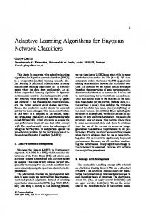
Fig. 1: Comparative scatter of No. of iterations (left), training time (middle) and RMSE (right) for NBw , NBd and NBe on All datasets (Top Row) and on Big datasets (Bottom Row). NBw on the X-axis, NBd (red-cross) and NBe (green-triangle) on the Y-axis.

the label represents this initialization. An absence of ‘(I)’ means the parameters are initialized to zero. 7.1 NB Structure Comparative scatter plots on all 72 datasets for 0-1 Loss, RMSE and training time values for NBw , NBd and NBe are shown in Figure 1. Training time plots are on the log scale. The plots are shown separately for Big datasets. It can be seen that the three parameterizations have a similar spread of RMSE values, however, NBw is greatly advantaged in terms of its training time. This computational advantage arises from the relative convergence properties of the three parameterizations and is discussed in Section 7.4. Given that NBw achieves equivalent accuracy with much less computation indicates that it is a more effective parameterization than NBd and NBe . The geometric means of the 0-1 Loss, RMSE and training time results are shown in Figure 2. Note, results are normalized with respect to NB, and, therefore, NB averaged results are all 1. They are also plotted on the graph for reference. Note, training time results are in log-scale. It can be seen that discriminative methods on Big datasets are an order of magnitude better than generative learning in terms of 0-1 Loss. Though discriminative training results in greatly improved 0-1 Loss and RMSE error, this gain in accuracy comes at a considerable cost in training time.

14

Nayyar A. Zaidi et al. 0-1 Loss

1.2 1 0.8

RMSE

1.2

NB w NB (I) NB d (I) NB e (I)

NB w NB (I) NB d (I) NB e (I)

1 0.8

0.6

0.6

0.4

0.4

0.2

0.2

10

4

10

3

Training Time NB w NB (I) NB d (I) NB e (I)

10 2

10 1

0

All

0

Big

All

10 0

Big

All

Big

Fig. 2: Geometric mean of No. of iterations, training time and RMSE for NB, NBw , NBd and NBe on All and Big datasets. Results are normalized with respect to NB.

0-1 Loss

1

RMSE

1

(I) (I), TAN

10 2

d

TAN

(I), TAN

0.4

TAN

d

0.6

10 0

TAN (I) TAN e (I)

TAN (I) TAN e (I)

0

0.2

0.4

0.6

0.8

0

1

0

0.2

0.4

0.6

0.8

10

-2

10

6

10

4

1

10 -2

10 0

TAN w (I)

TAN w (I) 0-1 Loss

1

TAN d (I) TAN e (I)

d

d

RMSE

1

10 4

Training Time

(I), TAN

10 2

10 0

0.2

0.2

TAN d (I) TAN e (I)

TAN d (I) TAN e (I)

0

0.2

0.4

0.6 TAN w (I)

0.8

1

10 6

d

0.4

TAN

TAN

d

0.4

0.6

TAN

(I), TAN

0.6

10 2 TAN w (I)

e

(I) e

e

(I)

(I)

0.8

0.8

(I), TAN

4

0.2

0.2

d

10

Training Time

e

(I) e

(I) e

(I), TAN

0.4

TAN

d

0.6

0

6

0.8

0.8

0

10

0

0

0.2

0.4

0.6 TAN w (I)

0.8

10 1

TAN d (I) TAN e (I)

-2

10 -2

10 0

10 2 TAN w (I)

10 4

10 6

Fig. 3: Comparative scatter of No. of iterations (left), training time (middle) and RMSE (right) for TANw , TANd and TANe on All datasets (Top Row) and on Big datasets (Bottom Row). TANw on the X-axis, TANd (red-cross) and TANe (green-triangle) on the Y-axis.

7.2 TAN Structure Figure 3 shows the comparative spread of 0-1 Loss, RMSE and training time of TANw , TANd and TANe on All and Big datasets. A trend similar to that of NB can be seen. With a similar spread of 0-1 Loss and RMSE among the three parameterizations, training time is greatly improved for TANw when compared with TANd and TANe . Geometric average of the 0-1 Loss, RMSE and training time results are shown in Figure 4. Note, results are normalized with respect to TAN, and, therefore, TAN averaged results are all equal to 1. They are also plotted on the graph for reference.

Efficient Parameter Learning of Bayesian Network Classifiers 0-1 Loss

1.2 1 0.8

RMSE

1.2

TAN w TAN TAN d TAN e

TAN w TAN TAN d TAN e

1 0.8

0.6

0.6

0.4

0.4

0.2

0.2

15

10

4

10

3

Training Time TAN w TAN TAN d TAN e

10 2

10 1

0

All

0

Big

All

10 0

Big

All

Big

Fig. 4: Geometric mean of No. of iterations, training time and RMSE for TANw , TANd and TANe on All and Big datasets. Results are normalized with respect to TAN.

0-1 Loss

RMSE

0.8

0.2 d

(I), KDB-1

0.4

0.2 KDB-1 (I) KDB-1 e (I)

0.8

0

0.2

0.4 0.6 KDB-1 w (I)

0.8

0.8

KDB-1

0.2 KDB-1 d (I) KDB-1 e (I)

0

0

0.2

0.4 0.6 KDB-1 w (I)

0.8

1

(I), KDB-1

0.4

0.2 KDB-1 d (I) KDB-1 e (I)

0

10

-2

KDB-1 d (I) KDB-1 e (I)

10

6

10

4

10 -2

10 0

10 2 KDB-1 w (I)

10 4

10 6

Training Time

10 2

d

d

0.4

0.6

KDB-1

(I), KDB-1

0.6

10 0

1

e

(I)

0.8

10 2

RMSE

1

e

(I), KDB-1 d

KDB-1

0

1

0-1 Loss

1

(I)

0.4 0.6 KDB-1 w (I)

4

(I)

0.2

e

0

10

Training Time

d

KDB-1 (I) KDB-1 e (I)

0

6

d

d

0.4

0.6

KDB-1

(I), KDB-1

0.6

KDB-1

KDB-1

d

(I), KDB-1

e

e

(I)

0.8

10 (I)

1

e

(I)

1

0

0.2

0.4 0.6 KDB-1 w (I)

0.8

10 0

10 1

KDB-1 d (I) KDB-1 e (I)

-2

10 -2

10 0

10 2 KDB-1 w (I)

10 4

10 6

Fig. 5: Comparative scatter of No. of iterations (left), training time (middle) and RMSE (right) for KDB-1w , KDB-1d and KDB-1e on All datasets (Top Row) and on Big datasets (Bottom Row). KDB-1w on the X-axis, KDB-1d (red-cross) and KDB-1e (green-triangle) on the Y-axis.

7.3 KDB (K = 1) Structure Figure 5 shows the comparative spread of 0-1 Loss, RMSE and training time of KDB-1w , KDB-1d and KDB-1e on All and Big datasets. Like NB and TAN, it can be seen that a similar spread of 0-1 Loss and RMSE is present among the three parameterizations of discriminative learning. Similarly, training time is greatly improved for KDB-1w when compared with KDB-1d and KDB-1e . Geometric average of the 0-1 Loss, RMSE and training time results are shown in Figure 6. Note, results are normalized with respect to KDB (K = 1), and,

16

Nayyar A. Zaidi et al. 0-1 Loss

1.2

KDB-1 w KDB-1 (I) KDB-1 d (I) KDB-1 e (I)

1 0.8

RMSE

1.2

KDB-1 w KDB-1 (I) KDB-1 d (I) KDB-1 e (I)

1 0.8

0.6

0.6

0.4

0.4

0.2

0.2

10

4

10

3

Training Time KDB-1 w KDB-1 (I) KDB-1 d (I) KDB-1 e (I)

10 2

10 1

0

All

Big

0

All

Big

10 0

All

Big

Fig. 6: Geometric mean of No. of iterations, training time and RMSE for KDB-1w , KDB-1d and KDB-1e on All and Big datasets. Results are normalized with respect to KDB-1.

therefore, KDB (K = 1) averaged results are all equal to 1. They are also plotted on the graph for reference. 7.4 Convergence Analysis A comparison of the convergence of Negative Log-Likelihood (NLL) of the three parameterizations on some sample datasets with NB, TAN and KDB (K = 1) structure is shown in Figure 7 and 8. In Figure 7, parameters are initialized to zero, whereas, in Figure 8, parameters are initialized to the log of the MAP estimates. It can be seen that for all three structures and for both ∗ initializations, MB faster but also reaches its asymptotic w not only converges ∗ B∗ value much quicker than the MB d and Me . The same trend was observed on all 73 datasets. ∗ To quantify how much MB w is faster than the other two parameterizations, ∗ ∗ we plot a histogram of the number of iterations it takes MB and MB e after d ∗ five iterations to reach the negative log-likelihood that MB w achieved at fifth iteration. If the three parameterizations follow similar convergence, one should expect many zeros in the histogram. Note that if after fifth iteration, NLL of ∗ ∗ of MB MB w is greater than that d , we we plot the ∗negative of the number ∗ B of iterations it takes MB w to reach the NLL of M d . Similarly, if after fifth ∗ B∗ iteration, NLL of MB is greater than that of M , we we plot the negative of w e ∗ ∗ the number of iterations it takes MB to reach the NLL of MB w e . Figures 9, 10 and 11 show these histogram plots for NB, TAN and KDB (K = 1) structure ∗ respectively. It can be seen that MB w (with all three structures) achieves a NLL that otherwise, will take on average 10 more iterations over the data for ∗ B∗ MB d and 15 more iterations for Me . This is an extremely useful property of B∗ Mw especially for big data where iterating through the dataset is expensive, but the more complex network structures are difficult to optimize. 7.5 Comparison with MAP The purpose of this section is to compare the performance of the discriminative learning with that of generative learning. In Table 3, we compare the

Efficient Parameter Learning of Bayesian Network Classifiers Localization

# 10 4

Census-income

-4.5 -5 -5.5 -6

-1.5

NB d NB e NB w

-5 Negative Log-Likelihood

Negative Log-Likelihood

-4

NB d NB e NB w

# 10 5

Covtype

-2

-6

-7

-8

-2

NB d NB e NB w

-2.5

-3

-3.5

-6.5

10 2

-9 10 0

10 3

10 1

Negative Log-Likelihood

Census-income

-6 -7 -8

-1

TAN d TAN e TAN w

-6.5 -7 -7.5 -8 -8.5

# 10 5

10 2 No. of Iterations

10 3

Localization

-5.5

KDB-1 d KDB-1 e KDB-1 w

10 1

# 10 4

10 2 No. of Iterations

10 3

NB d NB e NB w

-4 -5 -6 -7 -8

Negative Log-Likelihood

-6 -7 -8

10 4

10

2

10 No. of Iterations

10

3

10

4

-3

-4 -4.5 10 0

10 1

# 10 5

10 2 No. of Iterations

10 3

-7 -7.5 -8

10

2

10 No. of Iterations

10

3

10

4

Covtype

-3 -3.5

10

2

10 No. of Iterations

10

3

10

4

10 4

Poker-hand

-8 -10 -12

10 1

# 10 4

10 2 No. of Iterations

10 3

10 4

Poker-hand KDB-1 d KDB-1 e KDB-1 w

-4

-2

1

10 3

-6

-2

KDB-1 d KDB-1 e KDB-1 w

-2.5

-4.5 10 0

10 2 No. of Iterations

TAN d TAN e TAN w

-14 10 0

10 4

-4

1

# 10

10 1 4

-4

-3.5

-1

-6.5

-9 10 0

-2

TAN d TAN e TAN w

-1.5

-8.5

1

Covtye

-2

KDB-1 d KDB-1 e KDB-1 w

-10 10 0

10 4

-2.5

Census-income

-6

-5

-9 10 0

-9 10 0

10 4

# 10

5

10 3

-1.5

Negative Log-Likelihood

Negative Log-Likelihood

# 10

-6

-5

-4 Negative Log-Likelihood

-5.5

TAN d TAN e TAN w

4

10 2 No. of Iterations

Negative Log-Likelihood

Localization

10 1

10 1

No. of Iterations

-4

-9 10 0

-4 10 0

10 3

Negative Log-Likelihood

# 10

5

10 2

Negative Log-Likelihood

10 1 No. of Iterations

-3

Poker-hand

-9

-7 10 0

-3

# 10 4

-3 Negative Log-Likelihood

# 10 5

-4

Negative Log-Likelihood

-3.5

17

-6 -8 -10 -12 -14 10 0

10 1

10 2 No. of Iterations

10 3

10 4

Fig. 7: Comparison of rate of convergence on the four biggest datasets for NB (top row), TAN (middle row) and KDB (K = 1) (bottom row) structures. The X-axis is on log scale. Parameters are initialized to zero.

performance of NBw with NB (i.e., naive Bayes with MAP estimates of probabilities), TANw with TAN (i.e., TAN with MAP estimates of probabilities) and KDB-1w with KDB (K = 1) (i.e., KDB with MAP estimates of probabilities). We use NBw , TANw and KDB-1w as a representative of discriminative learning ∗ B∗ B∗ - since MB w , Md and Me have similar 0-1 Loss and RMSE profile. It can be see that the discriminative learning of parameters has significantly lower bias but higher variance. On big datasets, it can be seen that discriminative learning results in much better 0-1 Loss and RMSE performance. Note that though discriminative learning (optimizes the parameters characterizing CCBN) has better 0-1 Loss and RMSE performance than generative learning (optimizing joint probability), – generative learning has the advantage of being extremely fast as it incorporates counting of sufficient statistics from the data. Another advantage of generative learning is its capability of back-off in case a certain combination does not exist in the data. For example, TAN and KDB classifiers if have not encountered a < feature-value, parent-value, class-value > combination at training time can resort back to < feature-value, class-value > at testing time. For example TAN classifier can resort back to NB and NB can resort back to class prior probabilities. Such elegantly back-tracking is missing from discrimi-

18

Nayyar A. Zaidi et al. # 10 4

Census-income

-6.7766 -6.7766 -6.7766 -6.7766 -6.7766

-3.4

NB d (I) NB e (I) NB w (I)

-4 Negative Log-Likelihood

-6.7766

# 10 5

Covtype

-3.5

-5 -6 -7 -8

-8.5

NB d (I) NB e (I) NB w (I)

-3.6 -3.7 -3.8 -3.9

Localization

-8.02 -8.03 -8.04 -8.05

-8

# 10 5

10 2 No. of Iterations

-4 10 0

10 3

10 3

Census-income

10 1

-8.7 -8.8 -8.9

10 1

# 10 4

10 2 No. of Iterations

10 3

Negative Log-Likelihood

-8.02 -8.03 -8.04 -8.05

10 2 No. of Iterations

10 3

Covtype

-4.3 -4.4

10 1

# 10 5

10 2 No. of Iterations

10 3

-8.9

-8.9 -9

# 10

10 1 5

10 2 No. of Iterations

10 3

Poker-hand

-1.26 -1.28 -1.3 -1.32

-1.24

KDB1 d KDB1 e KDB1 w

10 1

# 10 5

10 2 No. of Iterations

10 3

-4.2 -4.25 -4.3 -4.35

10 4

Poker-hand KDB1 d KDB1 e KDB1 w

-1.26

-4.15

10 4

TAN d TAN e TAN w

-1.34 10 0

10 4

Covtype

-4.1

-8.8

-8.8

-1.24

-4.2

-4.05

-8.7

-8.7

-1.22

-4.1

-4

KDB1 d KDB1 e KDB1 w

NB d (I) NB e (I) NB w (I)

-9.2 10 0

10 4

TAN d TAN e TAN w

-4.5 10 0

10 4

Census-income

-8.6

# 10

5

-4

-8.6

-8.5

KDB1 d KDB1 e KDB1 w

-3.9

TAN d TAN e TAN w

-9 10 0

10 4

Localization

-8.01

# 10

-8.5 Negative Log-Likelihood

Negative Log-Likelihood

-8.4

TAN d TAN e TAN w

10 1

10 2 No. of Iterations

-8.01

-8.06 10 0

10 1 4

Negative Log-Likelihood

# 10

-9 10 0

10 2

Poker-hand

-9.1

Negative Log-Likelihood

-8

10 1 No. of Iterations 5

Negative Log-Likelihood

10 0

Negative Log-Likelihood

-6.7766

# 10 4

-8.6

-6.7766

Negative Log-Likelihood

Negative Log-Likelihood

-3

NB d (I) NB e (I) NB w (I)

Negative Log-Likelihood

Localization

-6.7766

Negative Log-Likelihood

# 10 5

-6.7766

-1.28 -1.3 -1.32 -1.34

-4.4 -8.06 10 0

10

1

2

10 No. of Iterations

10

3

10

4

-9 10 0

10

1

2

10 No. of Iterations

10

3

10

4

-4.45 10 0

10

1

2

10 No. of Iterations

10

3

10

4

-1.36 10 0

10 1

10 2 No. of Iterations

10 3

10 4

Fig. 8: Comparison of rate of convergence on the four biggest datasets for NB (top row), TAN (middle row) and KDB (K = 1) (bottom row) structures. The X-axis is on log scale. Parameters are initialized to the log of the MAP estimates.

NBw vs. NB W-D-L

p

Bias Variance 0-1 Loss RMSE

62/3/7