efficient performance prediction for modern ... - CiteSeerX

EFFICIENT PERFORMANCE PREDICTION FOR MODERN MICROPROCESSORS

A DISSERTATION SUBMITTED TO THE DEPARTMENT OF ELECTRICAL ENGINEERING AND THE COMMITTEE ON GRADUATE STUDIES OF STANFORD UNIVERSITY IN PARTIAL FULFILLMENT OF THE REQUIREMENTS FOR THE DEGREE OF DOCTOR OF PHILOSOPHY

David James Ofelt August 1999

Copyright © 1999 by David James Ofelt All Rights Reserved

ii

I certify that I have read this dissertation and that in my opinion it is fully adequate, in scope and quality, as a dissertation for the degree of Doctor of Philosophy.

__________________________________________ John L. Hennessy, Principal Advisor


__________________________________________ Kunle Olukotun


__________________________________________ Bruce A. Wooley

Approved for the University Committee on Graduate Studies:

__________________________________________

iii

Abstract Performance estimation of computer systems is an important topic to a large number of people in the computer industry. Computer architects need to be able to study future machines, compiler writers need to be able to evaluate the compiler output before a machine exists, and developers need insight into the machine’s performance in order to tune their code. There are many performance estimation techniques that range from profile-based approaches to full machine simulation. Detailed simulation is one of the most common methods for estimating performance. It suffers, however, from potentially long run times when simulating large applications using detailed processor models. This thesis discusses a profile-based performance estimation technique that uses a lightweight instrumentation phase that runs in order number of dynamic instructions, followed by an analysis phase that runs in order number of static instructions. This technique accurately predicts the performance of several pipelines including a detailed out-of-order issue processor model while scheduling far fewer instructions than does full simulation. The difference between the predicted execution time and the time obtained from full simulation is only a few percent. An extension to the basic technique accurately predicts branch prediction and instruction cache effects, but fails to handle data cache effects. Reasons for this failure are given. This thesis illustrates how this approach improves on earlier profile based analysis methods especially for the more advanced processor pipelines and illustrates how future processor trends will need new approaches.

iv

Acknowledgements There are a number of people I would like to thank for making my years at Stanford both extremely enjoyable and educational. First and foremost, I need to thank my primary advisor, John Hennessy, who gave me the opportunity and the freedom to pursue what I wanted to, and was always there to give me advice and guidance whenever I needed it. I would also like to thank the other two members of my reading committee Kunle Olukotun and Bruce Wooley both for their time and assistance in finishing this dissertation and also for being a pleasure to work with and around. This thesis grew out of a research project that Jeff Kuskin and I started many years ago at SGI. I would like to thank him for all his ideas and assistance in the early stages of this research. Besides Jeff, I also need to thank the people who contributed some of the tools and libraries that this research is based on. Jack Veenstra wrote MINT, the simulator infrastructure that underlies most of the run-time tools used here. Jeff Gibson wrote the cache simulator library used by the instrumentation tool and also the wonderful bargraph script that produced all the graphs in this thesis. Greg Steffan wrote Mintie, the program that generates the input trace for the R10000 simulator. Steve Turner was responsible for the R10000 simulator. He answered an enormous number of questions about the simulator and the R10000 over the years and has become a very good friend. Ken Yeager also fielded more than his fair share of questions about the processor. Finally, I would like to thank Earl Killian, who not only wrote the pixie tool, which was the best example of the “classic technique” presented in this thesis, but he also provided the core of the configurable pipeline simulator and he was a fantastic source of advice and ideas. My thesis may have had nothing to do with parallel computers, but I did spend most of my time at Stanford helping to build two. When I first arrived, I had the pleasure of helping to finish the DASH machine. I would like to thank Dan Lenoski, Jim Laudon, Truman Joe, Wolf-Dietrich Weber, Luis Stevens, Jaswinder Pal Singh, David Nakahira, and Anoop Goopta for making me welcome in the group and for teaching me what it takes to get a large hardware and software project successfully completed. The other machine I had the chance to work on was FLASH. Working with the FLASH team has been enormously enjoyable, and I look forward to working with all of

v

them again in the future. I would like to thank Jeff Kuskin, Mark Heinrich, John Heinlein, Joel Baxter, Dave Nakahira, Hema Kapeia, Jules Bergman, Ravi Soundararajan, Jeff Solomon, Jeff Gibson, Ziyad Hakura, John Hyuang, Dean Liu, David Lie, Richard Simoni, Richard Ho, Ricardo Gonzalez, Alan Swithenbank, and Mark Horowitz. Although we often lapse into a friendly hardware versus software rivalry, the SimOS/ Hive team has been a great fun to work with. I learned much of what I know about simulator and OS design by working with Steve Herrod, Robert Bosch, John Chapin, Dan Teodosiu, Kinshuk Govil, Ben Vergese, Scott Devine, and Ed Bugnion. I would like to thank the members of the MIPS architecture team Earl Killian, Pavlos Konas, Ruth Wilnai, Mike Gunter, Jack Veenstra, Steve Turner, Steve Herrod, Jeff Gibson, and Greg Steffan for being my group-away-from-Stanford. I really appreciate the work that Charlie Orgish, Thoi Nguyen, and Pat Burke did to kept the machines running and the bits safe. Margaret Rowland, Darlene Hadding, and Terry West always made sure I was paid and helped me recover from whatever administrivia disaster I managed to create for myself. Over the years, I have spent an inordinate number of hours talking to both Charlie and Margaret. They are two of the people that make Stanford a great place to be. Now and then, I did manage to have a life outside of Stanford. I would like to thank Chris Holt for being a good friend and putting up with me as a roommate for all these years, Anne Helgeson for her support and friendship through my hardest years at Stanford, and Ashley Saulsbury and Ing-Marie Jonsson for dragging me away from work when I really needed a break. I would also like to thank the other “roommates” I have had the pleasure of living with, Flora Lu, Gordon Stoll, Andrew Beers, and Diane Tang. My parents provided a huge amount of support over the years. They never really understood why it took so long to get a Ph.D., but were always there when I needed them. Finally, I would like to thank Beth Seamans, who is the greatest discovery I made in graduate school. Her patience and understanding during the long process of finishing this thesis made the task far less painful.

vi

Table of Contents Chapter 1 Introduction...................................................................................................1 1.1

Performance Prediction ................................................................................................................. 1 1.1.1 Motivation and Audience ........................................................................................................2 1.1.2 General Techniques .................................................................................................................2 1.2 Processor Trends............................................................................................................................ 5 1.3 Thesis Goal .................................................................................................................................... 7 1.4 Thesis Overview ............................................................................................................................ 7

Chapter 2 Classic Profile-Based Technique .................................................................9 2.1 2.2

Description..................................................................................................................................... 9 Results ........................................................................................................................................... 9 2.2.1 R5000 ....................................................................................................................................10 2.2.2 R10000 ..................................................................................................................................10 2.3 Why it Falls Short........................................................................................................................ 11 2.3.1 Relationship Between Instructions ........................................................................................12 2.3.2 Exceptions to the Normal Pipeline Flow...............................................................................17 2.4 Summary..................................................................................................................................... 18

Chapter 3 Methodology and Tools ..............................................................................19 3.1

3.2 3.3

3.4

3.5

Methodology................................................................................................................................ 19 3.1.1 Controlling Error ...................................................................................................................19 3.1.2 Evaluation Metrics.................................................................................................................21 Benchmarks ................................................................................................................................. 21 Simulators .................................................................................................................................... 23 3.3.1 R5000 ....................................................................................................................................23 3.3.2 R10000 ..................................................................................................................................24 Tools ............................................................................................................................................ 25 3.4.1 Instrumentation......................................................................................................................25 3.4.2 Analysis .................................................................................................................................26 Summary...................................................................................................................................... 27

Chapter 4 Pairwise Analysis Algorithm......................................................................28 4.1

4.2 4.3

4.4

4.5

Algorithm..................................................................................................................................... 28 4.1.1 Basic Algorithm.....................................................................................................................29 4.1.2 Arbitrary Analysis Depth ......................................................................................................31 4.1.3 Complexity ............................................................................................................................33 Methodology................................................................................................................................ 34 Accuracy Results ......................................................................................................................... 35 4.3.1 R5000 ....................................................................................................................................35 4.3.2 R10000 ................................................................................................................................36 Performance Results .................................................................................................................... 40 4.4.1 Instrumentation......................................................................................................................40 4.4.2 Analysis .................................................................................................................................40 Conclusions ................................................................................................................................. 45

Chapter 5 Pairwise Analysis Algorithm With Paths .................................................46 5.1 5.2

Path Tracing................................................................................................................................. 46 Path Data...................................................................................................................................... 47 5.2.1 Size of Code Objects .............................................................................................................48

vii

5.2.2 Complexity ............................................................................................................................48 Extending Base Algorithm With Paths........................................................................................ 51 Extensions to the Methodology ................................................................................................... 51 5.4.1 TInst.......................................................................................................................................51 5.4.2 TProf......................................................................................................................................52 5.5 Accuracy Results ......................................................................................................................... 52 5.5.1 R5000 ....................................................................................................................................52 5.5.2 R10000 ..................................................................................................................................55 5.6 Performance Results .................................................................................................................... 58 5.6.1 Instrumentation......................................................................................................................58 5.6.2 Analysis .................................................................................................................................58 5.7 Conclusions ................................................................................................................................. 64 5.3 5.4

Chapter 6 Extensions for Exceptional Pipeline Conditions ......................................66 6.1 6.2

6.3

6.4

6.5

Extensions to the Base Algorithm ............................................................................................... 66 6.1.1 Algorithm ..............................................................................................................................68 Extensions to the Methodology ................................................................................................... 69 6.2.1 TInst.......................................................................................................................................69 6.2.2 TProf......................................................................................................................................70 6.2.3 Robustness.............................................................................................................................70 Accuracy Results ......................................................................................................................... 71 6.3.1 Branch Prediction ..................................................................................................................72 6.3.2 Instruction Cache...................................................................................................................75 6.3.3 Data Cache.............................................................................................................................77 Performance Results .................................................................................................................... 83 6.4.1 Instrumentation......................................................................................................................83 6.4.2 Analysis .................................................................................................................................84 Conclusion ................................................................................................................................... 84

Chapter 7 Conclusion ...................................................................................................86 7.1 7.2

Summary and Conclusions .......................................................................................................... 86 Future Work................................................................................................................................. 88

References.........................................................................................................................90

viii

List of Tables Table 3.1

Integer benchmarks and their inputs ............................................................22

Table 3.2

Floating Point benchmarks and their inputs ................................................22

Table 6.1

Robustness Parameter Variations ................................................................71

ix

List of Figures Figure 1.1

Number of static and dynamic instructions per benchmark ...........................3

Figure 2.1

Accuracy of the classic technique on the R5000 pipeline ............................10

Figure 2.2

Accuracy of the classic technique on the R10000 pipeline ..........................11

Figure 2.3

Long dependency arcs ..................................................................................12

Figure 2.4

Super-scalar issue .........................................................................................14

Figure 2.5

Out-of-order issue .........................................................................................15

Figure 2.6

Pipeline startup .............................................................................................16

Figure 4.1

A base block and its successors ....................................................................29

Figure 4.2

The two schedules used by the algorithm .....................................................30

Figure 4.3

Arbitrary analysis depth................................................................................32

Figure 4.4

Number of traces for successor trace lengths of 0 to 64 instructions ...........33

Figure 4.5

BB-0 and BB-4 analysis error for the R5000 model ....................................35

Figure 4.6

Analysis error for the R5000 model using deeper analysis ..........................37

Figure 4.7

Analysis error for the R5000 model using BB-32 ........................................37

Figure 4.8

Analysis error for the R10000 model using BB-0 and BB-4........................38

Figure 4.9

Analysis error for the R10000 model using deeper analysis ........................39

Figure 4.10 Analysis error for the R10000 model using BB-32 ......................................39 Figure 4.11 Number of instructions scheduled for each successor trace length ..............41 Figure 4.12 Effectiveness of block pruning with various epsilons ..................................42 Figure 4.13 Effectiveness of arc pruning with various epsilons ......................................43 Figure 4.14 Block versus Arc pruning with an epsilon of 0.1% ......................................44 Figure 5.1

Example program flow graph .......................................................................47

Figure 5.2

Number of instructions per code object ........................................................48

Figure 5.3

Number of BBs and Paths per benchmark....................................................49

Figure 5.4

Number of traces generated for a collection of successor trace lengths .......49

Figure 5.5

Comparison of the number of traces for BB-32 versus Path-32...................50

Figure 5.6

Accuracy of BB-0 versus Path-0 on the R5000 model .................................53

Figure 5.7

Accuracy of Path-0 versus Path-4 on the R5000 model ...............................53

Figure 5.8

Accuracy of various successor trace lengths on the R5000 with Paths ........54

x

Figure 5.9

Accuracy of BB-32 versus Path-32 on the R5000 model .............................55

Figure 5.10 Accuracy of BB-0 versus Path-0 on the R10000 model...............................56 Figure 5.11 Accuracy of Path-0 versus Path-4 on the R10000 model .............................56 Figure 5.12 Accuracy on the R10000 model using several successor trace lengths ........57 Figure 5.13 Accuracy of BB-32 versus Path-32 on the R10000 model ...........................58 Figure 5.14 Scheduled instructions for each depth relative to the dynamic count...........59 Figure 5.15 Number of scheduled instructions for BB-32 versus Path-32 ......................60 Figure 5.16 Object pruning results for Path-32 over various values of epsilon...............61 Figure 5.17 Object pruning results for BB-32 versus Path-32 at an epsilon of 0.1% ......62 Figure 5.18 Arc pruning results for Path-32 over a variety of epsilons ...........................62 Figure 5.19 BB-32 versus Path-32 arc pruning with an epsilon of 0.1%.........................63 Figure 5.20 Object versus Arc pruning for Path-32 .........................................................64 Figure 6.1

Relative times of the branch prediction runs versus the perfect runs ...........72

Figure 6.2

Accuracy when predicting branch prediction effects using Path-32. ...........73

Figure 6.3

Delta time versus delta error for branch prediction and the base setup ........74

Figure 6.4

Robustness of the branch prediction estimate...............................................74

Figure 6.5

Relative execution time with the instruction cache effects...........................76

Figure 6.6

Accuracy of the prediction with instruction cache effects using Path-32.....76

Figure 6.7

Delta time versus delta error for the instruction cache effects .....................78

Figure 6.8

Robustness of the instruction cache prediction.............................................78

Figure 6.9

Relative execution time with the data cache effects .....................................79

Figure 6.10 Accuracy with the data cache effects using Path-32.....................................79 Figure 6.11 Delta time versus delta error for the data cache effects ................................80 Figure 6.12 Relative execution time with address effects................................................82 Figure 6.13 Accuracy with address effects using Path-32 ...............................................82

xi

1 Introduction Performance prediction of computer systems is an important topic to a large number of people in the computer industry. Computer architects need to study future machines, compiler writers need to evaluate the compiler output before a machine exists, and developers need insight into the machine’s performance in order to tune their code. There are many performance prediction techniques in use that range from statistics-based approaches to full system simulation. Detailed simulation is one of the most common methods for estimating performance. It suffers, however, from potentially long run times when simulating large applications using detailed processor models. This thesis introduces and evaluates a performance prediction technique that uses a lightweight instrumentation phase that runs in order number of dynamic instructions, followed by an analysis phase that runs in roughly order number of static instructions. The instrumentation phase only needs to run once per benchmark and the analysis phase runs once per benchmark per model under study. This technique accurately predicts the performance of several pipelines including a detailed out-of-order issue processor model. The difference between the predicted performance and the performance obtained from full simulation is only a few percent. An extension to the basic technique predicts branch prediction and instruction cache effects with reasonable accuracy, but fails to handle data cache effects. This thesis illustrates how this approach improves on earlier static analysis methods, especially for the more advanced processor pipelines and illustrates how future processor trends will need new approaches. This chapter will briefly introduce performance prediction: both who is interested and what techniques are available. Following this, it will introduce the rest of this thesis.

1.1 Performance Prediction Performance prediction is the generation of an estimate of the run time of a program on a given machine. The following two sections will introduce who is interested in performance prediction and what types of performance prediction are currently in use.

Introduction

1

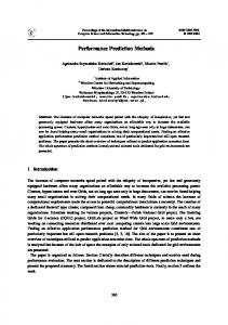
1.1.1 Motivation and Audience There are three general groups of people who are interested in performance prediction: architects, compiler writers, and developers. Computer architects demand the most detailed and the most flexible performance prediction tools, since they need to evaluate processors that do not yet exist. Once a basic architecture is established, performance prediction tools are used to explore and prune the parameter space for a design. Then, after the architecture is firm and physical design is underway, designers need sensitivity analysis for the various implementation decisions that need to be made. Compiler writers often develop a compiler for a processor before it exists. Performance prediction tools give them the ability to both determine if the compiler is functioning properly and to determine the performance of the code that is being generated. The final group, developers, needs performance prediction tools in order to analyze why their programs behave the way they do. Modern processors and systems are extremely complex, and tuning a piece of code in order to run fast on a given system is a difficult task. Performance prediction tools give the developer a way to discover where the time is being spent in a program and how they might be able to fix it. 1.1.2 General Techniques There are a large number of different performance prediction techniques from pure pencil-and-paper analysis to full machine emulation. This thesis concentrates on techniques that use data from runs of real benchmarks. These techniques can be sorted into two broad categories: the first is profile-based approaches and the second is simulationbased approaches. 1.1.2.1 Profile-Based Approaches Profile-based performance prediction approaches generally run a benchmark once under an instrumentation tool, generating average statistics for a given program run. Then, for each model under study, these statistics are fed into an analysis tool that uses the instrumentation data to calculate the estimate of the program’s run time. The instrumentation phase runs the entire program and is therefore proportional in cost to the number of executed instructions. Hopefully the profiling tool adds very little over-

Introduction

2

Static

Dynamic

log10(Instructions)

9.0 8.0 7.0 6.0 5.0 4.0 3.0 2.0

vpe

mxm

gmt

fft

emi

cho

btr

hydro2d

su2cor

swm256

mdljsp2

ear

alvinn

ora

tomcatv

wave5

mdljdp2

doduc

spice2g6

gcc

sc

compress

espresso

0.0

li

1.0

Benchmark

Figure 1.1 Number of static and dynamic instructions per benchmark head to the benchmark’s run time, making this process reasonably efficient. For the techniques used in this thesis, instrumentation adds only 15-30% to the benchmark’s run time. The analysis phase ideally needs to look at each instruction only once to generate the estimate of the program’s run time. This makes the cost of the analysis phase proportional to the number of static instructions. Figure 1.1 compares the static and dynamic instruction counts for the benchmarks used in this thesis. As with most of the graphs in this thesis, the benchmarks are listed along the X-axis with the integer benchmarks on the left and the floating point benchmarks on the right. The Y-axis in this graph gives the log base ten of the number of instructions. The left bar is the static instructions (the number of unique instructions executed) and the right bar is the number of dynamic instructions (the total number of instructions executed during the run). Even though these benchmarks use very small inputs, there are several orders of magnitude difference between the number of static instructions in the program text and the number of instructions actually executed. At their closest, these two counts only come within three orders of magnitude, and in some of the benchmarks they differ by as many as five orders of magnitude. Larger programs, with more realistic data sets will generate numbers with only a larger difference between the static and dynamic counts. The per-instruction analysis overhead is comparable to the per-

Introduction

3

instruction work a full simulator would incur. The overhead for the two simulators used to get the control numbers for this thesis is a factor of 400 to 13000. This shows the power of limiting the amount of work that needs to be done with every dynamic instruction. The earliest work on profiling was done by Knuth [K73][KS73]. More recently, some of the most common tools that implement profile-based performance prediction are Pixie/ Prof from MIPS [MIPS90], MTool from Stanford [GH93], QPT from the University of Wisconsin [L93], and also [S89]. These are the tools that were available during the 80’s and 90’s when the processors relevant to this thesis were being designed. After these came a number of tools that allowed a user to build an executable with custom instrumentation. These tools included ATOM from Digital [SE94], Shade from Sun [CK94], MINT from SGI [V97], and EEL from the University of Wisconsin [LS95]. These tools were not limited to building profile-based performance prediction, but this is one of the tasks they were used for. A study by Ball and Larus [BL94] showed that simple basic block node and edge profiling only added an average of 16% to the runtime of the uninstrumented application. This is a tiny overhead compared with simulation-based approaches, which at their fastest, are still an order of magnitude slower [WR96]. The analysis phase schedules the static instructions, to generate an estimate of their performance. This schedule is usually generated with a similar framework to the core of the processor simulator that generates timing. After this schedule is generated, it is combined with the information from the analysis phase to generate an estimate of the program’s performance. The per-instruction overhead of the analysis phase is therefore roughly the same as the per-instruction cost of a traditional simulator. Although they can be very efficient, profile-based tools have a number of weaknessesthese are discussed in §2.3. 1.1.2.2 Simulation-Based Approaches Simulation-based performance prediction techniques run every dynamic instruction of the benchmark through a program that models the architecture being studied. Since every instruction is simulated, the simulator can generate a very accurate prediction of the program’s performance. Unfortunately, this is also the drawback of simulators: they need to

Introduction

4

do substantial work for every dynamic instruction. There are many simulators currently being used in academics and industry, a sample are SimOS [RHW+95], SimICS [MDG+98], Talisman [B95], SimpleScalar [BA97], RSIM [PRA97], FastSim [SL98], and perft5 [T97] There are two main classes of simulators: emulators and trace-based simulators. An emulator actually executes the instructions in the program. This allows software to be tested on the simulator and also instills some confidence that if the applications run on the simulator, then the simulator is correct. A trace-based simulator runs off of a stored trace. A workload is run under an instrumentation tool very much like that needed by the profile-based approaches that generates a trace of important program events and saves them to a file. The simulator is then driven from the file. Trace-based simulation can be much faster than an emulator and it can give excellent repeatability. One drawback is that it is difficult to handle data dependent effects unless a huge amount of information is dumped to the trace and it is also impossible to have feedback from the timing model in the simulator affect the instruction stream.

1.2 Processor Trends During the past 15-20 years, there have been dramatic changes in the architecture of microprocessors. This time period can be roughly divided into three sections: the 1980s, the early 1990s, and the late 1990s. Processor pipelines and memory systems have both changed enormously during this time. For the purpose of this thesis, processors can be divided into two major pieces: the core processor pipeline and the memory system. Everything in between the core and the main memory is included in the memory system section.

1980s: During the 1980s processors had very simple pipelines. Two representative examples of processors from this era are the MIPS 2000 [KH92] and the Sun SPARC [GAB+88]. They usually issued a single instruction per cycle, and all instructions took either a single cycle to execute or were multi cycle but non pipelined. The memory systems were nearly all separable. If the memory system is separable, the processor pipeline can be simulated separately from the memory

Introduction

5

system and then the two results can be just added together to get the total runtime. The pipelines in early RISC microprocessors like the MIPS R2000 would block when a load or store missed in the cache. The pipeline would not restart until the memory system returned the data. The amount of concurrency in the processor was very low.

Early 1990s: In the early 1990s, processor architects started designing more sophisticated pipelines. Good examples of processors from this era are the MIPS R4000 [KH92], the MIPS R8000 [ITS+94], the MIPS R5000 [G96], the Sun SuperSPARC [AAB+92], the DEC ALPHA 21064 [DWA+92], and the DEC ALPHA 21164 [BAB+95]. Some processors could issue multiple instructions per cycle and the memory systems became more integrated into the processor pipeline than the previous generation. Designs during this period could manage to overlap some of the cache miss latency with useful instructions. Instruction fetch became more complicated and pipelines became deeper, so branch prediction started to be a common feature.

Late 1990s: The late 1990s are marked by very complex processors. Some good examples of the processors from this time period are the MIPS R10000 [Y96], the DEC ALPHA 21264 [GAB+97], the Sun UltraSPARC [CDd+95], and the Intel PentiumPro [CS95]. The pipelines are all multiple-issue, processors issue 2-4+ instructions per cycle, and the memory systems are all tightly integrated into the core pipeline. Many processor designs started to use out-of-order issue, which is a technique that hides latency by allowing instructions later in the program order to be executed before earlier (stalled) instructions. Most caches in the late 1990s are non-blocking.

The two processor models used in this thesis, the MIPS R5000 [G96] and the MIPS R10000 [Y96] are examples of early 1990s and late 1990s processors respectively.

Introduction

6

1.3 Thesis Goal Profile-based performance prediction techniques can be very efficient since they do a small amount of work for every dynamic instruction and limit the more expensive effort to the static instructions. Unfortunately, as §2.2 will demonstrate, classic profile-based techniques do not generate good performance estimates for modern microprocessors. The goal of this thesis is to develop a profile-based approach that can generate an acceptable estimate of a program’s performance on a given processor architecture in the face of the effects that §2.3 will present. The technique will use a lightweight instrumentation phase that runs in order number of dynamic instructions and an analysis phase that runs in roughly order number of static instructions. The ideal technique would be able to handle all architectural features that a given processor might have, but this is difficult to do all at once. This thesis will study processor features incrementally, first predicting the performance of the core pipeline, then it will move on to address more advanced features.

1.4 Thesis Overview This chapter introduced performance prediction: who is interested and what major methods are in use. The rest of this document will motivate, introduce, evaluate, and extend a new profile-based performance prediction approach. Chapter 2 introduces a classic performance prediction method, a profile-based technique that uses lightweight instrumentation to collect basic block frequency data from a run of the benchmark, and then uses an analysis phase that schedules each static basic block a single time to generate an estimate of the program’s run time. Unfortunately, this technique breaks down for modern processors and the results it generates are highly variable. There are a number of effects that the classic technique misses and these are all presented here. Chapter 3 introduces the basic methodology, the benchmarks, and tools used in the motivation section and as a base for the rest of the thesis. Each of the subsequent chapters will add to the methodology and tools, but they all build on the common base presented in this chapter.

Introduction

7

Chapter 4 describes the core contribution of this thesis, the Pairwise Analysis Algorithm. This algorithm builds on the classic profile technique by collecting both basic block counts and the counts of the arcs between basic blocks. Then, using this data to factor in the effects of the successors to a basic block as well the block itself, it generates an estimate of the block’s performance. The algorithm generates significantly more accurate performance estimates than the classic technique while retaining the efficiency advantages. The results of the Pairwise Analysis Algorithm from chapter 4 are very good, but it is possible to improve them by using an instrumentation technique called path tracing. Path tracing generates much longer sequences of instructions than plain basic block instrumentation with only slightly more work. Chapter 5 extends the Pairwise Analysis Algorithm to use path data instead of basic block data, thereby generating better performance estimates with less effort. The techniques in chapters 4 and 5 generate very accurate estimates of the performance of the core pipeline. Chapter 6 builds on this success and extends the Pairwise Analysis Algorithm to deal with three advanced processor features: branch prediction, instruction caches, and data caches. These extensions are reasonably successful at estimating the effects of the branch prediction and instruction cache effects, but fall short when dealing with data cache behavior. Finally, chapter 7 summarizes the thesis and discussions future work.

Introduction

8

2 Classic Profile-Based Technique The classic profile-based technique is used by Pixie/Pixstats [MIPS90], QPT [L93], and [S89] to generate an estimate of a program’s execution. This technique was developed and used during the architecture and design of the first generation RISC processors. Processor pipelines in this period were usually simple single-issue in-order designs.

2.1 Description The classic profile-based technique uses a two-phase approach. The first phase instruments the benchmark with code that counts the number of times each basic block executed during a specific run. The second phase schedules each basic block on a simple pipeline simulator and then multiplies this estimate by the number of times the block was executed. The sum of these results across all basic blocks gives an estimate of the total runtime of the program. This is shown more formally in equation 2.1. The execution time for a program, Tprogram, is the sum over all the basic blocks of the execution time for the basic block, Ti, times the number of times that block was executed, Counti. numBBs

Equation 2.1: T program =

å

T i · Count i

i=0

2.2 Results The classic technique works well on simple processor pipelines like the early MIPS processors [KH92]. For the most part, these processors have either single-cycle instructions or non-pipelined multi-cycle instructions. There is very little concurrency in the pipelines, so the problems that will be presented in §2.3 do not apply, and the classic technique will get acceptable accuracy. When more complicated processor pipelines are considered, such as the ones from the early and late 1990’s, the classic technique breaks down. The next two sections present data from using the classic technique on two modern processors– the MIPS R5000 and the MIPS R10000. Chapter 3 presents the methodology used to collect the data presented here. After these results, §2.3 discusses the reasons for the inaccuracies.

Classic Profile-Based Technique

9

2.2.1 R5000 The MIPS R5000 [G96] has a simple dual-issue 5 stage pipeline. On each cycle, an integer or memory operation can be issued with a floating point operation. Throughout this thesis, the R5000 model will just focus on the core pipeline: the caches are always perfect. The R5000 did not have a branch predictor, so that is also not an issue. Figure 2.1 presents the accuracy of the classic technique when analyzing the R5000 pipeline. The benchmarks are listed along the X-axis and the Y-axis indicates the error introduced by the performance estimate generated by the classic technique. The accuracy is expressed as the percent difference between the performance estimate for the benchmark and the time the benchmark took on a detailed simulator of the processor. If the estimate is longer than the real execution time, then the accuracy will be positive. If the estimate is shorter, then the accuracy will be negative. With one exception the classic technique’s prediction always undershoots the actual performance. The standard error (see §3.1.2) is only 7.82% but the individual benchmark errors range from -20.5% to +1.16% which is quite a large variation. 2.2.2 R10000 The MIPS R10000 [Y96] is an out-of-order issue super-scalar microprocessor. It can issue and retire four instructions per cycle. The processor has a large number of functional

Figure 2.1 Accuracy of the classic technique on the R5000 pipeline

5.0

Error (%)

0.0 -5.0 -10.0 -15.0


STE

vpe

fpppp

gmt

mxm

fft

emi

cho

btr

hydro2d

su2cor

mdljsp2

swm256

ear

alvinn

ora

wave5

tomcatv

doduc

mdljdp2

spice2g6

sc

gcc

li

compress

-25.0

espresso

-20.0

Benchmark

10

250

Error (%)

200 150 100

STE

vpe

fpppp

gmt

mxm

fft

cho

emi

btr

hydro2d

su2cor

mdljsp2

swm256

ear

alvinn

ora

wave5

tomcatv

doduc

mdljdp2

spice2g6

sc

gcc

li

compress

0

espresso

50

Benchmark Figure 2.2 Accuracy of the classic technique on the R10000 pipeline units that allow many instructions to be in flight concurrently. It uses branch prediction to reduce the instruction fetch penalty of branches. The primary instruction cache is 32KB and is two-way set associative. The primary data cache is also 32KB and is a lock-up-free writeback cache. For this thesis the secondary cache is always perfect. Figure 2.2 shows the results of using the classic technique to predict the performance of the SPEC92 benchmarks. Instead of consistently undershooting the performance like the R5000 model, the prediction here always overshoots. The standard error is huge at 125% and the individual benchmark errors range from 19.6% to 246%.

2.3 Why it Falls Short There are a number of reasons why the classic profile technique does not achieve good accuracy on either the R5000 or the R10000 pipelines. Generally, there are two different types of pipeline events that are missed. The first are caused by the relationship between instructions. These events are unavoidable in the normal functioning of the pipeline, and they include structural limitations to issue and also data dependent effects that change the flow of instructions in the pipeline. The second type of event are exceptional events. These happen much less frequently than the events caused by the relationship between instructions. Since the processor models used to generate the results in the previous sections do not model any of the excep-


11

tional events, these are not the cause of the classic technique’s errors. They are discussed here, since they need to be addressed by a technique that is seeking to replace as much full simulation as possible. Chapter 6 will introduce techniques to address these effects. The following two sub-sections describe these two types of effects in more detail. 2.3.1 Relationship Between Instructions The following sections will give examples of the pipeline behaviors caused by the relationship between instructions that lead to inaccuracies in the classic technique. All of these are present in the data from the previous results, although not all effects are present in both processor models. 2.3.1.1 Long Dependency Arcs One major source of missed cycles with the classic technique is long dependency arcs that extend between basic blocks. Dependency arcs that are completely contained within a basic block that cause a dependent instruction to stall will be properly accounted for. On the other hand, if a dependent instruction is in a succeeding basic block, there is no mechanism to account for the proper number of stall cycles since only a single block is analyzed at a time. Figure 2.3 shows an example of this problem. Here, there are two basic blocks BB1 and its successor block BB2 (figure 2.3A). The first block has an integer

Figure 2.3 Long dependency arcs

BB1

0 add

r1,r2,r3

0 add

r1,r2,r3

0 add

r1,r2,r3 r1,r2

add

r1,r2,r3

1 div

r1,r2

1 div

r1,r2

1 div

div

r1,r2

2 add

r1,r2,r3

2 add

r1,r2,r3

2

3 add

r1,r2,r3

3 add

r1,r2,r3

3

4 add

r1,r2,r3

4 add

r1,r2,r3

4

BB2 add

r1,r2,r3

5

add

r1,r2,r3

6 mfhi r1

add

r1,r2,r3

5 mfhi r1

mfhi r1

5 6 add

r1,r2,r3

7 add

r1,r2,r3

8 add

r1,r2,r3

9 mfhi r1

A Classic Profile-Based Technique

B

C

D 12

divide, which for this example takes five cycles. The instruction that uses the result of the divide is in the second basic block. Figure 2.3B shows the correct schedule for these two blocks. Notice that the mfhi instruction stalls for one cycle waiting for the divide to finish. The classic technique has no way of accounting for this stall, since the divide instruction is in a different basic block than the use of the result. Figure 2.3C shows the result of using the classic technique with a scheduler that considers an instruction complete as soon as it has issued. This behavior is the same as the R5000 model used in this thesis. With this scheme, two cycles of stall are missed. The R10000 model considers an instruction completed when it graduates. This will generate the schedule shown in Figure 2.3D. This case has the dependency arc for the divide completely contained within the first block. This is wrong as well, since the real schedule has some cycles of overlap between the two blocks. The end result is that, depending on the semantics of the pipeline scheduler being used, the classic technique will either over estimate the number of cycles or under estimate the number of cycles. 2.3.1.2 Super-Scalar Issue Modern high-performance processors all issue multiple instructions in a cycle. This ability is called super-scalar issue. There is a good chance that a basic block will not completely fill all the issue slots on its final cycle; the left over slots can be filled by instructions from the succeeding block. The classic technique will not account for this overlap; therefore, it will overestimate the number of cycles it would take to execute the two blocks. Figure 2.4 shows an example. The processor here has a dual issue pipeline that can issue adds simultaneously to both sides of the pipeline. Each of the basic blocks in figure 2.4A has three independent instructions. All six instructions will issue in three cycles on a real pipeline, since the unused slot from the first block can be filled with an instruction from the second block. The classic technique, however, will generate the schedule shown in Figure 2.4C. Since it is unable to account for the overlap between the two blocks, the two blocks take an extra cycle to execute.


13

BB2 add

r1,r1,r1

add

r2,r2,r2

add

r3,r3,r3

0 add

r1,r1,r1 add

r2,r2,r2

1 add

r3,r3,r3 add

r7,r7,r7

2 add

r8,r8,r8 add

r9,r9,r9

B BB2

0 add

r1,r1,r1 add

r2,r2,r2

add

r7,r7,r7

1 add

r3,r3,r3

add

r8,r8,r8

2 add

r7,r7,r7 add

add

r9,r9,r9

3 add

r9,r9,r9

A

r8,r8,r8

C

Figure 2.4 Super-scalar issue 2.3.1.3 Out-Of-Order Issue A technique that is used by a large number of recent processors is out-of-order issue. This technique allows instructions to be issued to the functional units out of program order. Independent instructions can then fill in the gaps caused by stalls between dependent instructions, causing two basic blocks to effectively bleed together, executing in possibly much less time than they would have in isolation. Since the classic technique can only deal with the blocks in isolation, it will miss all cycles of overlap that might be present. Figure 2.5A shows two basic blocks. The first block has a divide and an instruction that uses the result of the divide. Assuming the divide takes five cycles, there will be four cycles of stall between these two instructions. The second basic block contains four independent adds. Figure 2.5B shows the proper schedule on a single-issue out-of-order issue machine. The adds from the second basic block can all be issued during the stall cycles between the div and the mfhi and the result is that both blocks can execute in the same number of cycles as the first block could alone. The classic technique deals with basic blocks in isolation, so it can not account for the overlap and generates the schedule shown in figure 2.5C.


14

BB1 div

r1,r2

mfhi r3

BB2

0 div

r1,r2

0 div

1 add

r4,r4,r4

1

2 add

r5,r5,r5

2

3 add

r6,r6,r6

3

4 add

r7,r7,r7

4

5 mfhi r3

r1,r2

5 mfhi r3

add

r4,r4,r4

add

r5,r5,r5

6 add

r4,r4,r4

add

r6,r6,r6

7 add

r5,r5,r5

add

r7,r7,r7

8 add

r6,r6,r6

9 add

r7,r7,r7

A

B

C

Figure 2.5 Out-of-order issue 2.3.1.4 Pipeline Startup Pipelines take several cycles between fetching an instruction from the instruction cache and actually executing it. If the processor model being analyzed takes these cycles into account, then this is another effect that the classic technique can miss. For two examples in §2.2, the R5000 model only deals with the execute stage of the pipeline, it does not model the instruction fetch part. Therefore, it does not have any pipeline startup effects. The R10000 model, on the other hand, models all phases of an instruction’s execution including instruction fetch. This causes a several cycle stall at the beginning of any schedule while an instruction moves through the stages of the pipeline before issue. Once the pipeline starts up, the early stages are all overlapped with previous instructions. The classic technique deals with each basic block in isolation, and generates a fresh schedule for each. This means that there are several cycles of stall at the beginning of each basic block that would not be present if the blocks were scheduled together. The classic technique will therefore cause the number of cycles to be overestimated. Figure 2.6A shows two simple basic blocks. Assuming these are scheduled on a classic five stage pipeline (figure 2.6B)[HP96], then it takes three cycles for the first instruction to start executing: one cycle each for instruction fetch (IF), instruction decode (ID), and register fetch (RF). The correct schedule for the two blocks is given in 2.6C. The star-


15

BB1

0

0

add

r1,r2,r3

1

1

add

r4,r5,r6

2

2

3 add

r1,r2,r3

3 add

r1,r2,r3

4 add

r4,r5,r6

4 add

r4,r5,r6

BB2 add

r7,r7,r7

5 add

r7,r7,r7

5

add

r8,r8,r8

6 add

r8,r8,r8

6

A IF

C ID

7 8 add

r7,r7,r7

9 add

r8,r8,r8

RF EX WB D B

Figure 2.6 Pipeline startup tup cycles for the second block are completely overlapped with the first block. The classic technique generates the schedule shown in figure 2.6D. Each block is charged the full startup cost, since each is scheduled in isolation. 2.3.1.5 Data Dependent Effects The final relationship between instructions that is missed by the classic technique is data dependent effects. There are many of these in a modern processor design. For example, an integer divide may take a different number of cycles depending on the actual operands being used. Another type of data dependent effect is due to the interaction between load and stores. In many processors, loads can bypass stores in order to generate cache misses as early as possible. This is only safe to do if a load is to a cache line different from all currently outstanding stores. If a load is trying to issue, and it does target a different cache line from any outstanding store, then it can issue immediately. Otherwise, if it targets the same line as a current store, then it will need to stall until the store data is generated. The classic technique has no way of dealing with data dependent effects. It uses a single schedule for a block, possibly missing the several other legal schedules that would occur with different operands or addresses. In the examples presented in §2.2, there are no


16

data dependent effects because the pipeline models do not have any, but in chapter 6 these will have a large effect 2.3.2 Exceptions to the Normal Pipeline Flow The previous section introduced a number of effects that are present in normal pipeline flow. This section presents some additional effects that are very important from a performance standpoint, but can best be viewed as exceptional conditions. Each of these causes an interruption in the normal pipeline flow of possibly a large number of cycles. They are all strongly data and context dependent, so more information is needed to address them than just the program’s instructions. 2.3.2.1 Branch Prediction Modern processors have deep pipelines and therefore have several cycles of latency between fetching a branch and actually determining what the branch target actually is. To prevent a several cycle penalty for each branch, these processors all include a branch predictor. This is a piece of hardware that takes some information about the current branch and often information about the previous branches and generates a prediction of whether the branch will be taken or not. These predictions are not always correct and when they are wrong, or mispredicted, the pipeline has to back up and re-fetch instructions from the actual destination instead of the mispredicted destination. A misprediction usually costs between one and ten cycles of stall. 2.3.2.2 Instruction Cache There are tens to hundreds of cycles of latency between main memory and the processor core. This memory is not only many cycles away, it also has limited bandwidth. All modern processors include a small fast memory close to the core of the chip that holds instructions that can be accessed in a single cycle and has enough bandwidth to feed the processor’s instruction demands. This memory is called an instruction cache. As long as the processor needs instructions that are in the instruction cache, there is no penalty for access. If, on the other hand, the processor requests an instruction that is not present, then there will be many cycles of delay while the instructions are fetched from a lower level of cache or main memory.


17

2.3.2.3 Data Cache The processor needs to access data efficiently as well as instructions, so all modern processor designs include a data cache. If a load or store targets data that is present in the cache, then the instructions can execute with no penalty. If the data is not present, then there will be many cycles of delay while it is fetched from a lower level of the memory hierarchy. The most advanced processors use lock-up-free caches. These allow several cache misses to be in flight at the same time and also allow instruction execution to overlap with the memory fetches. This feature significantly increases the amount of concurrency in the normal pipeline operation. 2.3.2.4 Other Exceptional Conditions There are many other exceptional conditions that affect a processor’s performance, including TLB effects, real exceptions, interrupts, etc. These are all beyond the scope of this thesis.

2.4 Summary This chapter introduced the classic profile-based performance estimation technique and evaluated its performance on two modern processor pipelines. It then presented the major sources of error that the classic technique missed. The next chapter introduces the methodology used in this chapter and as a basis for the rest of the studies in this document.


18

3 Methodology and Tools The previous chapter introduced the classic profile-based technique and presented data to show that this technique does not handle modern pipelines well. This chapter presents the framework used to perform the experiments in chapter 2, and provides a basis for the methodology used in the rest of this document. There are three major topics introduced here: the basic methodology, the benchmarks, and the tools. Each of these is discussed in the following sections.

3.1 Methodology The goal of this thesis is to introduce and evaluate an algorithm to efficiently estimate the execution time of a program on a given processor architecture. If the algorithm is successful, then the difference between the real runtime and the predicted runtime will be very small. In order to measure these small errors reliably, it is necessary for the experimental setup to introduce little or no error itself. The other condition for the algorithm’s success is that it is efficient. The following section discusses how experimental error is limited and how the accuracy and performance of the algorithms are evaluated. 3.1.1 Controlling Error Ideally, the estimate of a benchmark’s performance on the desired architecture is compared to the real running time of the same program on a real instance of the architecture under study. Unfortunately, a comparison to a real machine has two major problems: it is hard to fix variables and there is poor visibility into the internal workings of the system. The ability to fix variables is a key necessity to do a scientific experiment. All variables except for the one currently under study need to be known and held constant. If they are not then two problems occur: the first is that measurement error is added to the final result and the second is that the repeatability of the experiment is poor. The addition of measurement error distorts the most important metric the experimental framework analyses. Poor repeatability makes it hard to generate consistent result and to do related sets of experiments. Limited visibility is the other major problem with real hardware. Most systems have some performance monitoring hardware in the processor but only a fixed set of resources

Methodology and Tools

19

and events can be measured. If the current problem being studied requires insight into a feature that is not covered by any of the performance hardware, then there is probably no way to find the needed information. Because of these two major shortcomings, this thesis uses detailed simulators to generate the control numbers for the processors under study. Simulators allow all variables to be fixed and controlled at will and they also provide great visibility into the system. Additionally, if a study needs to add or change one of the current simulator knobs or if there is not yet enough visibility into a key part of the simulator, these features can be added. These simulators fix all the variables that might cause problems in the various studies. For the results in chapters 2, 4, and 5 the branch predictor is fixed to be perfect, the instruction and data caches to always hit, and all data dependent effects are turned off. In chapter 6, branch prediction and the cache effects will be turned on individually. In this chapter the only important data dependent effect that will be enabled is the address behavior in the R10000 pipeline. Programs execute slightly different instructions every time they execute due to I/O and other interactions with the OS and hardware. This variability is nearly impossible to eliminate, so the methodology used here sidesteps the issue by using a single run of a program to generate both the control numbers and the instrumentation numbers needed by the analysis phase. This removes the variability between runs as a source of error. All tools that need to execute a benchmark are based on MINT [V97], giving them a much more constant environment, and therefore ensuring that the results are similar from run to run. One final thing that is done to reduce error is that all the benchmarks are run from start to finish. This limits the studies here to benchmarks that have relatively short runtimes since the full simulators are not very fast. Often, techniques such as sampling are used to reduce the runtime of full simulation: these work well and are used extensively in the field. Unfortunately, sampling introduces a source of error since the samples run for the study may not fully represent the exact behavior of the full benchmark. The error introduced is usually small, but since the algorithm being evaluated will hopefully have a small error, this additional error is unacceptable.


20

3.1.2 Evaluation Metrics The two aspects of a performance estimation algorithm that need to be evaluated are the accuracy and the efficiency. Both of these are measured relative to a full simulation of the studied benchmark. Accuracy is simply the difference between the benchmark’s execution time on the simulator and the execution time estimate generated by the performance estimation algorithm. If the estimate is larger than the real runtime, then the error will be positive. If the real runtime is larger than the estimate, then the error will be negative. All accuracy results present the standard error as a way of showing what the “average” error across the benchmarks. The standard error is computed by taking the square-root of the average of the squared errors for each of the benchmarks. In the various accuracy graphs, the standard error is always the right-most bar and is labeled “STE.” The other metric used to evaluate the algorithm is efficiency. Using the runtime of the new estimation tool versus the runtime of the simulator is the obvious way to evaluate the efficiency of the technique. Unfortunately, this is a hard approach to measure fairly, since it depends strongly on the amount of time and effort spent tuning the various tools. A metric is needed that is free from implementation details. Thankfully, there is a natural one in this context: the number of instructions analyzed by each of the techniques. The core of both the classic algorithm and the algorithm proposed in this thesis is a piece of code that needs to take a block of instructions and generate the number of cycles it would take on the processor being studied. This process is identical to the core of the full simulator. The difference is that the efficient estimation algorithms just schedule small blocks of code from the static text, where the full simulation approach schedules all the dynamic instructions in the full run of the program. If the efficient algorithm is successful, then it will schedule fewer instructions than full simulation.

3.2 Benchmarks As section 3.1.1 discussed, every instruction in the benchmarks must be executed so as not to introduce error from sampling or other speedup techniques. The SPEC92 benchmarks [SPEC92] are a set of realistic programs that are used to evaluate microprocessor designs. Most of these have a reasonable runtime for the default data set. For the ones that


21

do not, a smaller data set or number of iterations is used. The integer benchmarks are listed in table 3.1 and the floating point benchmarks are in table 3.2. The input used for each benchmark is listed in the second column. All graphs that list the benchmarks along the X-axis will have the integer benchmarks on the left side and the floating point benchmarks on the right. Note that 093.nasa7 is split into its seven different kernels. These kernels are all independent and have quite different behavior. Running them all together as a single benchmark would obscure the results. These benchmarks are all compiled with the SGI 7.2 compiler with the following options “-n32 -mips4 -r10000 -LNO:prefetch=0”. Table 3.1 Integer benchmarks and their inputsa Benchmark

Input

008.espresso

from input.ref - ti.in

013.spice2g6

greycode.in (short version)

015.doduc

doduc.in (small version) tlim=35

022.li

input.short (queens 8)

026.compress

input file is 100000Bytes

a. A bug in one of the simulators prevents 023.eqntott from running correctly.

Table 3.2 Floating Point benchmarks and their inputs Benchmark

Input

034.mdljdp2

input.short - 100 steps (vs. 1000)

039.wave5

3 iterations (vs. 5)

047.tomcatv

-

048.ora

input.short (15200 vs. 456000 iterations)

052.alvinn

50 epochs (vs. 200)

056.ear

args.short

072.sc

input.short/load1

077.mdljsp2

input.short - 100 steps (vs. 1000)


22

Table 3.2 Floating Point benchmarks and their inputs Benchmark

Input

078.swm256

input.short - 60 iterations (vs. 1200)

085.gcc

stmt.s

089.su2cor

input.short - 2 iterations (vs. 50)

090.hydro2d

input.short (50 vs. 400 iterations)

093.nasa7.btr

5 iterations (from 20)

093.nasa7.cho


093.nasa7.emi


093.nasa7.fft


093.nasa7.gmt

default

093.nasa7.mxm


093.nasa7.vpe

100 iterations (vs. 400)

094.fpppp

input.short (8 atoms)

3.3 Simulators This thesis uses two processor simulators, one for the MIPS R5000 and the other for the MIPS R10000. These processors are good representatives of early and mid 1990’s processors respectively. The next two sections will introduce the simulators used to model each of them. 3.3.1 R5000 Section 2.2.1 introduced the MIPS R5000 architecture. The simulator used in this thesis to model the R5000 is called pipesim, and only models the core pipeline from issue through completion. The caches, TLB behavior, etc. are all perfect and are not modelled. The memory system in the R5000 is separable; that is, when the processor takes a cache miss, the pipeline is stalled until the cacheline comes back from the memory system. This property allows the memory behavior to be modelled by a separate simulator, and then the effects can be just added into the execution time determined by the pipeline simulator.


23

Pipesim accurately models the dual-issue constraints, resource constraints, and functional unit latencies and throughput. It is built on top of MINT in order to insure the same execution characteristics as the other tools. Pipesim is a flexible simulator that can model a large variety of superscalar processors. The pipeline description comes from an input file that specifies available functional units. Each instruction has an entry that specifies which of the functional units it needs along with a collision vector [D71] which is a bit vector where each bit represents a specific cycle that resource is needed. The simulator keeps a similar vector for each functional unit that indicates which cycles that resource is busy in the future. Using this information makes scheduling an instruction an easy operation. If the resource bit vectors needed by an instruction do not conflict with the busy vectors for each of the needed functional units, then the instruction can be scheduled. If no instruction can be scheduled, then time is stepped forward and all the functional units busy vectors are shifted by one bit. This scheme is flexible enough to model pipelined or non-pipelined functional units, complex resource dependencies between functional units (e.g. the integer divider needs one of the ALUs for a cycle at the beginning and at the end of the divide), and a wide variety of processor configurations. The pipeline configuration used in pipesim to model the R5000 processor was written by the chief R5000 architect [K97] and it accurately models the details of that processor’s pipeline. All of the issue constraint, functional unit latencies, and resource restrictions are modelled accurately. 3.3.2 R10000 The R10000 model used in this thesis is called perft5, and it is the main architectural model used by SGI/MIPS for the design of the R10000 processor. This model is accurate to within a few percent of the real hardware [T97]. Perft5 is a trace-driven simulator. Although it is trace-driven, it tries to be intelligent about mispredicted branches. The simulator has access to the program text, so it will actually simulate the instructions down the mis-predicted speculative path. Being trace-driven, it is not able to form the proper addresses for any speculative memory operations that


24

might occur, so just picks an arbitrary address. In practice the simulator generates accurate results, so this approximation does not seem to be a problem. The trace input is from a pixie-format [S91] trace generator called mintie. Instead of the traditional trace generators used by SGI/MIPS (pixie or mixie), mintie is based on MINT. This gives it a similar instruction execution behavior to the other tools used in this thesis. There are a large number of knobs that allow the user to control all aspects of perft5. This thesis configures the model to be as close to the R10000 as possible, and then only controls the behavior of the branch predictor, instruction cache, data cache, and some data dependent effects. The only other parameter set that differs from the standard R10000 is one that causes the instruction queues to always issue oldest instructions first. This does not have much of effect on absolute accuracy, but it causes the results to be more consistent and repeatable. For chapters 2, 4, and 5 perft5 is configured to have perfect branch prediction, instruction cache behavior, data cache behavior, and no data dependent effects due to addresses. The address effects are due to locking for index and bank conflicts. The locking is to prevent deadlock and livelock conditions that arise when speculative loads and stores conflict on cachelines needed by older instructions that have not yet graduated. This locking is necessary for the load-store unit to function correctly, so it is not possible to run the model with real data cache behavior but with ideal address effects. It is valid, however, to turn on address effects without turning on realistic cache behavior. Chapter 6 will individually turn on realistic branch prediction, instruction caching, data caching with realistic address effects, and finally, just realistic address effects.

3.4 Tools There are many tools used in this thesis, but the two most important ones are the instrumentation and analysis programs that collect the program statistics and generate the final performance estimates respectively. 3.4.1 Instrumentation TInst is the instrumentation tool used to generate all the program statistics needed by the analysis phase. It is written on top of MINT, for the same reasons as the previous tools.


25

TInst generates output files that contain all the information about a specific run of a benchmark including all the instructions, library information, information about the procedures executed, and in chapter 2 information about the basic blocks. Each of the results chapters adds to the information collected by TInst. In chapter 2, it just discovers basic blocks and counts how many times each was executed. Chapter 4 extends this slightly by also discovering the arcs between blocks and their counts. A much larger change is made in chapter 5, where information on specific paths and the path frequency for the program is collected as well as the arcs and arc frequency between paths. Finally, in chapter 6, simple branch prediction, instruction cache, and data cache simulators are added to TInst to collect detailed information about the behavior of these features. All analysis is done with the information collected by TInst. In order to compare the results of analysis to the control numbers on a finer grained basis than just the total execution time of the benchmark, TInst folds in the timing information from the control runs. Both the pipesim and perft5 simulators can output a stream of consisting of the PC of an instruction and the cycle it completed on, and then TInst gathers this information in the same granularity that the analysis will be done on. For the basic block-based analysis, it will collect the amount of time spent in the control run for each basic block. In the pathbased analysis, it collects the amount of time spent in each path. If the execution time generated by the analysis phase does not match the time from the control run, it is now possible to find the specific blocks that are responsible for the most contributed error. 3.4.2 Analysis All analysis is done by a program called TProf. This program takes the data generated by TInst and generates an estimate of the program’s run time either with the classic technique from chapter 2 or the techniques presented in chapters 4, 5, and 6. TProf needs to be able to generate an estimate of the run time of blocks of instructions on the target architecture. In order to not add another source of error, the exact same simulators used to generate the control numbers are used by TProf in the analysis phase. Each of the two simulators is integrated with TProf in a different way. The core of pipesim is a library that implements the instruction scheduler; the MINT instrumentation routines


26

make references to this library to schedule each instruction. The same interface is used by TProf when it needs to figure out how many cycles an instruction took. The interface to perft5 is more complicated. The simulator is not structured in a way that made it easy to generate a library with a simple interface. Instead, TProf runs perft5 as a separate process and feeds it with synthetic pixie traces. For each block of code that TProf needs to schedule, it generates a pixie trace that is nearly identical to what mintie would generate if that sequence of instructions were run under MINT. It is extremely inefficient to spawn off a perft5 for each block of instructions that needs to be scheduled, so TProf does all scheduling with a single instance of perft5. In order to isolate different blocks from each other, a block of separator instructions is fed to the simulator between each set of instructions to be scheduled. This separator block contains an instruction that serializes the R10000 pipeline to cause all instructions ahead of it to finish, then a block of NOPs long enough to fill the entire reorder buffer. The NOPs prevent instructions from the next block from starting until the previous block has completely finished. This approach is reasonably efficient and generates repeatable results.

3.5 Summary This chapter introduced the basic methodology used in this thesis and presented the benchmarks on which the algorithm is tested. This methodology tries to reduce the error in the experimental framework since the goal of the thesis is to measure potentially very small errors in the new algorithm. Three things lead to a small experimental error: the first is that all the variables are fixed, giving repeatability and observability. The second is that the same simulators are used to generate the control numbers as well as the instruction schedules for the performance estimation algorithm. Finally, the control information is collected in the same granularity as the analysis is done: allowing analysis errors to be tracked in a fine-grained way. The next chapter presents the Pairwise Analysis Algorithm. This algorithm tries to overcome the accuracy limitations of the classic technique while still retaining the performance benefits.


27

4 Pairwise Analysis Algorithm Chapter 2 introduced the classic analysis technique and demonstrated that its accuracy falls short because it misses a number of important pipeline effects. The execution time estimates it generated were in some cases too optimistic and in others, overly conservative. The solution is to analyze multiple basic blocks at a time. This chapter introduces the Pairwise Analysis Algorithm which addresses the shortcomings of the classic technique by using the successors of a block as well as the block itself to generate the estimate of the execution time. It then evaluates how well the algorithm works in both accuracy and in number of instructions scheduled. The chapter concludes with a summary of the results.

4.1 Algorithm A technique that analyses multiple basic blocks must take into account the stall that a block (the base block) has on a successor block, the stall that a successor block imparts onto the base block, and the overlap between blocks. A dependency arc that extends from an instruction in the base block to an instruction in a successor block will cause additional cycles of stall, thereby making the successor basic block take more time. In an out-oforder issue processor, instructions from the successor block can be scheduled before instructions in the base block, causing the base block to take longer to execute. Finally, successor instructions can be pipelined with base instructions or can fill empty issue slots left by the base instructions, thereby causing both blocks to run faster together than each would in isolation. A basic block can have multiple successors, so the algorithm must take into account the effects of each successor on the base block individually. Then it must combine these into a single estimate for the execution time for the base block. The following two subsections describe the basic algorithm and an extension to the algorithm that uses arbitrary numbers of successor instructions to improve the execution time estimate.

Pairwise Analysis Algorithm

28

4.1.1 Basic Algorithm Chapter 2 introduced the algorithm used by the classic technique. This algorithm generates an estimate for the run time of each basic block in the program, multiplies this estimate by the number of times the block was executed, and then sums the result over all the basic blocks. This is shown formally in Equation 4.1. The execution time estimate for the program, Tprogram, is the sum of the products of Ti, the execution time estimate for basic block i, and Counti, the number of times that basic block was executed. numBBs

å

Equation 4.1: T program =

T i · Count i

i=0

The Pairwise Analysis Algorithm extends the classic technique by making the calculation of the basic block time (Ti) take into account the effect of its successor blocks. Figure 4.1 shows a basic block and its successors. Each of the successors has a normalized frequency of fi, where all the fi for a basic block will sum to 1.0. The algorithm deals with each of the successor blocks individually and then does a weighted sum of the results to generate the estimate for the base block. Figure 4.2 shows this. Ti is the estimate for the base basic block i, fij is the frequency of the arc between blocks i and j, and eij is the estimate of the time the base basic block taking into account the effects of its successor, j.

Figure 4.1 A base block and its successors

Base

numSuccs

f0 Succ0


f1 Succ1

å

fn

f i = 1.0

i=0 Succn

29

numSuccs

Equation 4.2: T i =

å

f ij · e ij

j=0

The heart of the algorithm is in the calculation of eij. This value is the sum of two different times (see Equation 4.3), the first, ti, is the time it took the base block to execute when run with the successor block. The second time, sij, is the number of extra cycles it took the successor block to execute when it was scheduled with the base block. If the successor block took longer to execute, for example due to a long dependency arc from the base block, then this will be a positive quantity. If super-scalar or out-of-order issue effects allowed the successor block to be overlapped with the base block causing it to take less time to execute than it would on its own, then this will be a negative addition. Equation 4.3: e ij = t i + s ij The quantity sij is easy to calculate. It is simply the difference between the number of cycles it took the successor block to execute when scheduled with the base block and the number of cycles it took the successor block to execute in isolation. Figure 4.2 shows two schedules: the first, Schedule 1, has both the base and successor blocks scheduled together, and the second, Schedule 2, is just the successor block scheduled alone. Schedule 1 gives two times: baseTime and succTime. The baseTime is the time from cycle 0 until the last instruction of the base block completes. Then, succTime is the number of cycles from the last base instruction completion to the last successor instruction completion. The

Figure 4.2 The two schedules used by the algorithm

Schedule 1

B0

Bn

baseTime

Schedule 2

S0

S0

Sn

succTime

Sn

succOnlyTime


30

time for the successor block in isolation is calculated the same as the baseTime. When these terms are combined, they result in the full equation for sij given in equation 4.4. This equation makes sense, since it will result in a stall time of zero if the base block had no effect on the successor block. In this case, the succTime will be the same as the succOnlyTime. It will yield a positive stall time if the successor block takes longer to execute when scheduled with the base block, and a negative stall time if the two blocks were successfully overlapped. Equation 4.4: s ij = ( t ij – t i ) – t j When equations 4.3 and 4.4 are combined with equation 4.2, some of the terms cancel, and the result is equation 4.5. This is the final form that is used to generate an estimate the execution time of a block. In English, this reads that the execution time for a block is the weighted sum over all the successors of the time for the block scheduled with one successor minus the successor scheduled in isolation. numSuccs

Equation 4.5: T i =

å

f ij · ( t ij – t j )

j=0

4.1.2 Arbitrary Analysis Depth The previous description of the algorithm used pairs of basic blocks. There is no reason that longer sequences of blocks cannot be used. Multiple successors (successors of


31

successors) can be combined into a large block with an arc frequency that is adjusted accordingly. Figure 4.3 shows a base block, its successors, and one of the successors’s successors. In this example Succ0 and Succ0,0 can be combined into a new successor that has an arc frequency of (fo•g0). This new block can be used in the pairwise analysis algorithm just like the normal successor block was before in section 4.1.1. There is no reason that this is limited to a depth of two successors; the process can be continued indefinitely. Eventually, though, the benefits of going deeper in the call graph will level off. This is due to two reasons, the first being that adding more instructions to the schedule will not cause the pipeline effects to change significantly between the shorter and the longer traces. The second is that the approximation to the real call graph represented by the traces being assembled will get worse the deeper into the call graph the algorithm goes [BL96]. Dealing with sequences of successors based on integral numbers of basic blocks is an arbitrary granularity. It makes more sense to count instructions instead, so rest of this thesis will use sequences of N instructions from the successor blocks. These sequences are called successor traces. This chapter constructs traces from basic blocks, the next chapter will construct the same trace using a more powerful instrumentation technique. Here a successor trace is constructed by taking enough basic blocks from the successor blocks to achieve a successor trace of the proper length. Now, the algorithm will use the base basic Figure 4.3 Arbitrary analysis depth

Base

f0 Succ0

g0 Succ0,0


Base

fn

f1

f0g0

Succ1

Succn Succ0

g1 Succ0,1

gn Succ0,n

Succ0,0

32

block and the successor trace as the pair of objects used to generate the execution time estimate for the base block. 4.1.3 Complexity When longer traces of successor instructions are used, the number of traces increases dramatically. This is due to the fact that as more basic blocks are needed to supply the instructions, the algorithm must go deeper into the flow graph. Every branch point in the flow graph causes the current trace to split into a new trace for each of the successors. This results in the number of traces that is potentially exponential in the depth of the search. Worst-case exponential growth is bad, but in practice the number of traces (and hence the number of instructions analyzed) is reasonable for the sizes of traces that produce acceptable accuracies. Figure 4.4 shows the number of traces analyzed for a variety of successor trace lengths. There are seven bars for each benchmark along the X-Axis; each one indicates the number of traces generated when the analysis uses a successor trace of the given number of instructions. Trace length is varied from zero to 64 instructions. The Yaxis gives the log base 10 of the number of traces for the given successor trace length. It is clear from the graph that the number of traces is a strong function of the length of the trace. The growth is exponential in the depth of the trace and it grows as the depth to the Figure 4.4 Number of traces for successor trace lengths of 0 to 64 instructions bb-0

bb-4

bb-8

bb-16

bb-32

bb-48

bb-64

log10(Num Traces)

9.0 8.0 7.0 6.0 5.0 4.0 3.0 2.0


fpppp

vpe

gmt

mxm

fft

emi

cho

btr

hydro2d

su2cor

swm256

mdljsp2

ear

ora

alvinn

tomcatv

wave5

doduc

mdljdp2

spice2g6

sc

gcc

compress

li

0.0

espresso

1.0

Benchmark

33

1.17. Chapter 5 will introduce an instrumentation technique that has a much shallower growth curve. With the basic block data, a successor trace length of 48 instructions generates about a million traces for most benchmarks. This corresponds to 50 to 60 million instructions scheduled for each benchmark, or an order of magnitude less than the dynamic instruction count. Section 4.11 will give more data on this and show ways of reducing the number of instructions by adding controlled amounts of error. A successor trace length of 32 instructions is a good practical maximum trace length for this study. At this length the number of instructions analyzed for each benchmark will be less than the dynamic instruction count, with only one exception. The one problem benchmark improves dramatically with the technique presented in §4.4.2.2 and with this technique, the number of instructions analyzed drops below the number executed for all benchmarks.

4.2 Methodology The basic methodology used in this chapter is nearly identical to that of the classic study presented in chapter 2. The only difference is that TInst now collects the information required by the Pairwise Analysis Algorithm and TProf uses this algorithm when generating the run-time estimate. In the classic study, TInst collected just basic block counts. The Pairwise Analysis Algorithm needs information about the arc frequencies between the basic blocks as well as the block counts. To get this information, TInst now generates the full basic block flow graph and counts not only the number of times each block executes, but also the number of times each arc between blocks is taken. In chapter 2, TProf just used the classic analysis technique and only analyzed a single basic block at a time. For the study in this chapter, TProf obtains an estimate for a block’s execution time with the Pairwise Analysis Algorithm (§4.1.1), scheduling a block with each of its successor traces. These traces are generated using the additional basic block arc data from TInst. The results in this chapter are presented as BB-n. The “BB” means that the data used by the analysis phase is based on the basic-block flow graph generated by the instrumentation phase. Chapter 5 will introduce an instrumentation technique that will generate the flow graph a different way and there, the “BB” prefix will be necessary to differentiate the


34

bb-0

bb-4

5.0

Error (%)

0.0 -5.0 -10.0 -15.0

STE

fpppp

vpe

gmt

mxm

fft

emi

cho

btr

hydro2d

su2cor

mdljsp2

swm256

ear

alvinn

ora

wave5

tomcatv

mdljdp2

doduc

spice2g6

sc

gcc

compress

li

-25.0

espresso

-20.0

Benchmark

Figure 4.5 BB-0 and BB-4 analysis error for the R5000 model current technique with the new technique. This chapter uses the same naming scheme for consistency. The other part of the name, “n”, is the number of instructions in the successor trace. The classic technique has no instructions in the successor trace, so it will appear as BB-0. This means that the base basic block is scheduled with a zero-length successor trace. The simulator parameters are the same as for the classic study. The R5000 pipeline model is unchanged, and the R10000 model again just models the base pipeline while the cache, branch prediction, and address behaviors are ideal.

4.3 Accuracy Results This section presents the accuracy studies for the Pairwise Analysis Algorithm on both the R5000 and the R10000 processor models. These results show that the new algorithm generates significantly better results than the classic technique, although there is still room for improvement. 4.3.1 R5000 Figure 4.5 shows the results of using the Pairwise Analysis Algorithm on the R5000 pipeline. The graph presents the benchmarks along the X-axis and the percent error along


35

the Y-axis. As in Chapter 2, the errors are positive if the performance estimates overshoot and negative if they fall short. For each benchmark, there are two bars: BB-0 and BB-4. Here, the BB-0 data is identical to that presented in §2.2.1 and represents the classic technique of analyzing a single basic block at a time. The BB-4 data is the result of using the Pairwise Analysis Algorithm scheduling with a successor trace length of four instructions. The results show that in all cases but one, the BB-4 results are superior to the classic technique. The standard error dropped from 7.81% to 4.75%. The single exception is swm256 due to small scheduling noise, and will improve with longer successor traces. Figure 4.6 presents the accuracy of the Pairwise Analysis Algorithm using longer traces. The results of the classic technique are not shown on this graph, since the larger errors overshadow the bars from the longer traces. The results continue to improve as the traces become longer, with all but two of the benchmarks reaching nearly 0% error with 32 instructions in the successor trace. The results for just BB-32 appear in figure 4.7. All of the bars are essentially nearly a 0% error, except for 034.mdljdp2 and 089.su2cor. Both of these benchmarks have exactly the same problem: a long dependency arc that is not captured by a successor trace of 32 instructions. In both benchmarks there are very long basic blocks of 40+ instructions that have a divide late in the block. These blocks are part of a software pipelined loop, so the instruction that depends on the divide does not appear until late in the next iteration. A successor trace of 40 instructions is needed to capture this arc, and when the analysis is done with a successor trace of this length, the error for both benchmarks drops to zero. 4.3.2 R10000 The R10000 results for BB-0 and BB-4 appear in figure 4.8. The improvement in accuracy is even more dramatic than in the R5000 case. Much of the gain here is due to the fact that the pipeline startup time is being accounted for. The standard error dropped dramatically from 125.65% to 17.34%. Figure 4.9 shows how analysis error improves with increasing successor trace length. As before, the data from the classic technique (BB-0) is left out so as to not obscure the rest of the data. In all the benchmarks save two, the error decreases monotonically with increasing depth. The two exceptions are fft and mxm.


36

-16.0


mdljsp2

-10.0

-12.0

-14.0 ora

fft

emi

cho

btr

hydro2d

su2cor

swm256

mdljsp2

ear

alvinn

STE

-8.0 fpppp

-6.0

STE

-4.0 vpe

-2.0

fpppp

0.0 mxm

2.0

vpe

4.0 gmt

Figure 4.6 Analysis error for the R5000 model using deeper analysis

gmt

Benchmark

mxm

fft

emi

cho

btr

hydro2d

su2cor

swm256

wave5 tomcatv

bb-16

ear

alvinn

ora

tomcatv

mdljdp2

doduc

spice2g6

gcc

sc

compress

li

Error (%)

bb-8

wave5

mdljdp2

doduc

spice2g6

gcc

sc

compress

li

espresso

-20.0

espresso

Error (%)

bb-4 bb-32

5.0

0.0

-5.0

-10.0

-15.0

Benchmark

Figure 4.7 Analysis error for the R5000 model using BB-32

37

bb-0

bb-4

250

Error (%)

200 150 100 50

STE

fpppp

vpe

gmt

mxm

fft

emi

cho

btr

su2cor

hydro2d

swm256

ear

mdljsp2

alvinn

ora

tomcatv

wave5

doduc

mdljdp2

spice2g6

sc

gcc

compress

li

-50

espresso

0

Benchmark

Figure 4.8 Analysis error for the R10000 model using BB-0 and BB-4 Both mxm and fft have the same general problem: almost all the execution time is in a small number of basic blocks that each take a small number of cycles. In the case of mxm, there are three basic blocks that each take on average 8.5 cycles and in the case of fft, there are 8 blocks that each take 8 cycles. Noise in the scheduler, due to initial conditions or the exact point the successor trace was truncated, can easily cause plus or minus one cycle of scheduler error. This is, in fact, what is happening for these two benchmarks. Longer successor traces tend to alleviate the problem, since longer traces of instructions can drive the pipeline model into a closer approximation of steady state. The error for both of these benchmarks stabilizes with a successor trace length of more than 32 instructions. Another way of improving the accuracy is to increase the size of the base block, since this will cause a single cycle of scheduler noise to be much less significant. The technique introduced in chapter 5 will help the accuracy of these benchmarks by doing just that. Figure 4.10 presents just the BB-32 accuracy results. This shows clearly that the analysis errors are very low, in all but two cases less than 5% and one of those two is only 5.55%. The standard error is only 3.76%. The remaining benchmark, mxm, has a larger error of 16.37% caused by the problems just discussed.


38

-5.0


mdljsp2

ora

fpppp STE

STE

fft

emi

cho

btr

hydro2d

su2cor

swm256

mdljsp2

ear

alvinn

vpe

0.0

fpppp

5.0

mxm

10.0

vpe

15.0

gmt

Figure 4.9 Analysis error for the R10000 model using deeper analysis

gmt

Benchmark

mxm

fft

emi

cho

btr

hydro2d

su2cor

swm256

wave5 tomcatv

bb-16

ear

alvinn

ora

tomcatv

mdljdp2

doduc

spice2g6

gcc

sc

Error (%)

bb-8

wave5

mdljdp2

doduc

spice2g6

gcc

sc

compress

li

espresso

-30

compress

li

espresso

Error (%)

bb-4 bb-32

30

20

10

0

-10

-20

Benchmark

Figure 4.10 Analysis error for the R10000 model using BB-32

39

4.4 Performance Results The previous section demonstrated that the Pairwise Analysis algorithm generates very accurate estimates of a program’s performance on both processor models. This section evaluates the run-time performance of the algorithm. As described in §2.1, the performance estimation process is divided into two pieces, the instrumentation phase and the analysis phase. The next two subsections evaluate the run-time performance of each of these phases independently. 4.4.1 Instrumentation The instrumentation phase is proportional to the total number of dynamic instructions in the program, this puts a strong requirement that overhead of the instrumentation to be small. Ball and Larus [BL94] report that for the SPEC95 benchmarks, their efficient edgebased profiling technique only causes an average 16% overhead over the run time of the uninstrumented program. The fastest simulator has a factor of four to ten times slowdown just to execute the instructions [WR96]. The two simulators used in this thesis, pipesim and perft5 have slowdowns of 400 and 13000 times respectively. By contrast, the instrumentation overhead is insignificant when compared to these. 4.4.2 Analysis As §3.1.2 discussed, the only fair way to evaluate the run-time performance of the analysis phase is to just look at the number of instructions scheduled. This section presents the performance of the analysis phase, then introduces and evaluates two methods of reducing the number of scheduled instructions. 4.4.2.1 Base Figure 4.11 shows the number of instructions scheduled for several different successor trace lengths. The X-axis has six bars for each benchmark: the left bar is the static instruction counts respectively, and the five on the right give the results of ramping the successor trace length from zero to 32 instructions. The Y-axis gives the log base 10 of the number of scheduled instructions relative to the dynamic instruction count. The average number of instructions scheduled for a successor trace of 32 instructions is 52 times fewer than the number of dynamic instructions. 085.gcc analyses slightly more (9.8%) instructions than


40

were executed, but this problem improves with the pruning techniques presented in the next two sections. 4.4.2.2 Block Pruning The previous section shows that a very large number of instructions need to be analyzed when deeper analysis is performed. These results performed the Pairwise Analysis Algorithm on every block in each benchmark. Fortunately, programs spend most of their time in a small number of blocks [K71]. One way to reduce the number of instructions analyzed would be to only analyze the basic blocks that contribute the most to the execution time. Pruning out the infrequent blocks adds a small amount of error to the result, but potentially a large amount of work can be skipped. Unfortunately, the number of cycles a block takes to execute is not known until the analysis is done. A heuristic is needed that will give an approximate weighting to the blocks that closely matches the weighting derived using the number of cycles. One heuristic that works well is to use the number of instructions contributed by the block. If one block represents more executed instructions than another it does not necessarily mean that the first block takes more cycles to execute, but in practice, it turns out to be an acceptable approximation. Figure 4.11 Number of instructions scheduled for each successor trace length bb-0

bb-4

bb-8

bb-16

bb-32

0.0 -1.0 -2.0 -3.0 -4.0


vpe

fpppp

mxm

gmt

fft

cho

emi

btr

hydro2d

su2cor

mdljsp2

swm256

ear

alvinn

ora

wave5

tomcatv

mdljdp2

doduc

spice2g6

gcc

sc

compress

-6.0

li

-5.0

espresso

log10(Norm sched instrs)

Static

Benchmark

41

The pruning algorithm used here is simple. All the basic blocks are sorted by the number of contributed instructions. The blocks that contribute the fraction (1- e) of the total instructions are then used in the Pairwise Analysis to generate the estimate of the execution time. The number of instructions analyzed relative to the dynamic instruction count for each of four different epsilons, 0%, 0.01%, 0.1%, and 1% are shown in Figure 4.12. The static instruction count relative to the dynamic count is shown as the left bar. All of the benchmarks show a substantial savings in the number of instructions analyzed. On average, an epsilon of 0.1% schedules 895 times fewer instructions than full simulation and 17 times fewer instructions than the base technique. The one problem block in the previous section, gcc, now has the number of analyzed instructions drop below the dynamic instruction count by 43%. The difference between e and the actual error introduced by the pruning when using a e

of 0.1% and a successor trace length of 32 instructions, was only 0.018% for the R5000

and 0.039% for the R10000. These small differences support the validity of the pruning heuristic.

Figure 4.12 Effectiveness of block pruning with various epsilons 0.000

0.010

0.100

1.000

0.0 -1.0 -2.0 -3.0 -4.0


vpe

fpppp

mxm

gmt

fft

emi

cho

btr

hydro2d

su2cor

swm256

ear

mdljsp2

alvinn

ora

tomcatv

wave5

mdljdp2

doduc

spice2g6

gcc

sc

compress

-6.0

li

-5.0

espresso


Static

Benchmark

42

0.000

0.010

0.100

1.000

0.0 -1.0 -2.0 -3.0 -4.0

vpe

fpppp

mxm

gmt

fft

cho

emi

btr

hydro2d

su2cor

swm256

mdljsp2

ear

alvinn

ora

tomcatv

wave5

mdljdp2

doduc

gcc

spice2g6

sc

compress

-6.0

li

-5.0

espresso


Static

Benchmark

Figure 4.13 Effectiveness of arc pruning with various epsilons

4.4.2.3 Arc Pruning The previous result showed that pruning infrequent objects is quite effective at reducing the number of instructions that need to be scheduled. A better result is obtained by focusing on the arcs between blocks instead of the blocks themselves. Each arc in the flow graph represents a certain number of instructions, namely its frequency multiplied by the number of dynamic instructions in the base block. The arcs can be sorted by contributed instructions exactly as the blocks were in §4.4.2.2. Only the arcs that contribute the fraction (1-e) of the dynamic instructions are analyzed; all the other arcs are pruned out. Figure 4.13 presents the arc pruning results for the same epsilons as figure 4.12. As with the block-based pruning, the results improve dramatically with increasing values of epsilon. Here, the arc-based pruning approach with an e of 0.1% gives an average savings of 5856 times over full simulation and 106 times fewer than the base technique. The heuristic performs here just as well as for the previous results: the maximum difference between the actual error introduced and epsilon is only 0.016% for the R5000 model and 0.037% for the R10000 model. The final graph, figure 4.14, presents a side-by-side comparison between the block and the arc-based pruning techniques for an epsilon of 0.1% and a successor trace length of 32


43

Full

Obj

Arc

0.0 -1.0 -2.0 -3.0 -4.0

vpe

fpppp

mxm

gmt

fft

cho

emi

btr

hydro2d

su2cor

swm256

mdljsp2

ear

alvinn

ora

tomcatv

wave5

mdljdp2

doduc

gcc

spice2g6

sc

compress

-6.0

li

-5.0

espresso


Static

Benchmark

Figure 4.14 Block versus Arc pruning with an epsilon of 0.1% instructions. For each benchmark, it shows the static instruction count, the number of instructions analyzed when the full analysis is done, the number of instructions analyzed for block and arc pruning all relative to the dynamic instruction count. The arc pruning algorithm analyzes far fewer instructions compared to the block pruning algorithm. On average arc pruning analyzes 6.54 times fewer instructions than does block-based pruning and 5855 times fewer than the dynamic instruction count, a significant savings. Full simulation requires the same amount of work per instruction as the analysis phase, so the Pairwise Analysis Algorithm here is substantially faster than full simulation and is nearly as accurate. The drawback of the arc pruning technique is that it requires all the traces to be enumerated and weighed so the pruning can happen. If the flow graph is very large and the analysis is being done with a large successor trace length, the number of traces will get very large and will take up a significant amount of memory and may cause the arc pruning technique to be impractical. The future work section proposes an adaptive technique that will prune out insignificant blocks, then work on pruning out the insignificant arcs.


44

4.5 Conclusions The Pairwise Analysis Algorithm dramatically improves the prediction accuracy for both the R5000 and the R10000 models. The standard error dropped to 3.18% and 3.76% respectively. Not only is the analysis accurate, it also is efficient. With no optimizations, the analysis phase schedules 52 times fewer instructions than does full simulation. Pruning techniques make it even more efficient, dropping the number of instructions scheduled to 5855 times fewer than full simulation while adding less than 0.15% additional error. The results are better than the classic technique, but there are two remaining problems with the current technique. The first is the base blocks are not long enough. They are not able to adequately warm up the processor pipeline, especially in the case of the R10000. Long successor traces can help with this problem, but a single cycle of noise results in a large analysis error when the base block is only a few cycles long. The second problem is with generating the successor traces. This problem has two components. First, there is exponential growth in the number of paths as the successor trace gets larger. Second, the match between this successor trace and the real flow graph gets worse as the flow graph gets larger. The next chapter introduces a technique called path tracing that generates much longer sequences of instructions with only slightly more overhead than basic block profiling. When the pairwise analysis algorithm is extended to use this new data, the results improve significantly while scheduling fewer instructions.


45

5 Pairwise Analysis Algorithm With Paths The previous chapter introduced a technique that generates good results for both the R5000 and the R10000 pipelines, but there is room for improvement. There are two problems with the Pairwise Analysis Technique when it is based on basic blocks: the instruction traces for the base objects are too short and the number of scheduled instructions grows as the successor trace length increases. This chapter presents a technique called Path Tracing that generates longer instruction sequences, allowing the base technique to get better accuracy while analyzing fewer instructions. This chapter introduces path tracing, gives some motivational data, and then presents the accuracy and performance results when the path data is incorporated into the analysis. These results show that the instruction data from path tracing improves the accuracy of the Pairwise Analysis Algorithm while analyzing fewer instructions for the same successor trace length.

5.1 Path Tracing Path Tracing is a technique that counts unique paths through a piece of code instead of just counting the basic blocks. The most recent work on the topic was done by Ball and Larus [BL96]. They demonstrated that path data could be collected for only slightly more overhead than collecting basic block data. A path is an acyclic sequence of instructions through a program that may span many basic blocks. An example program flow graph is shown in figure 5.1. It consists of seven basic blocks labeled “A” through “G”. The flow graph has two conditional blocks causing two forks and joins. The instrumentation done in the previous chapter would treat all these blocks and the arcs between them as separate entities. With path tracing, instead of seven blocks, there are only four paths: ABDEG, ABDFG, ACDEG, ACDFG. These same paths can be approximated from the basic block data by generating sequences of multiple basic blocks using the arc frequency between blocks. These traces only approximate the real flow graph since the amount of correlation between the arcs out of A and the arcs out of D is unknown. The path data, however, gives an exact flow graph.

Pairwise Analysis Algorithm With Paths

46

A 90

10

B

C D 90

10

E

F

Path

Real Freq

BB Freq

ABDEG

90

81

ABDFG

0

9

ACDEG

0

9

ACDFG

10

1

G Figure 5.1 Example program flow graph Figure 5.1 shows a contrived example to illustrate the problem. In this example, there are only two paths of execution actually taken when the program is run, ABDEG and ACDFG. The other two paths are not executed at all, since the branches in A and D are completely correlated. The “Real Freq” column in the table shows the real execution frequencies for the paths. If just the basic block arc frequency is used to try and reconstruct the path frequencies, there is no way of knowing that the branches in A and D are correlated. The results of using the basic block arc frequency data is shown in the “BB Freq” column. Not only is there is a large difference between the estimated and actual path frequencies for the paths that were really executed, the two paths that didn’t execute are assigned non-zero frequencies. This chapter uses the term code object to refer to both basic blocks and paths when the discussion needs to talk about both techniques or when the exact source of the data does not need to be specified.

5.2 Path Data The benefit of path tracing is that it generates code objects with longer sequences of instructions than does basic block counting. One potential drawback is that since there are now many branches in each path, there is an exponential number of possible paths. This could lead to an explosion of the number of paths seen during a program run, but in practice this does not happen.


47

Instrs/BB

Instrs/Path

Avg Instructions

60 50 40 30 20

vpe

mxm

gmt

fft

emi

cho

btr

hydro2d

su2cor

swm256

mdljsp2

ear

alvinn

ora

tomcatv

wave5

mdljdp2

doduc

spice2g6

gcc

sc

compress

espresso

0

li

10

Benchmark

Figure 5.2 Number of instructions per code object 5.2.1 Size of Code Objects Figure 5.2 is a graph of the average number of instructions per code object for each of the SPEC92 benchmarks. The code objects shown are basic blocks and paths. Paths are significantly longer than basic blocks. They range from 2.88 to 13.5 times longer and the average path is 4.57 times longer than the average basic block. 5.2.2 Complexity There is a potential explosion in the number of paths for a program due to the fact that a single path may contain several branches. Since each of these branches has at least two possible outcomes, there is the possibility of a huge number of paths. In practice, this does not happen, since most of the branches in the program always have the same destination, and the number of paths actually seen during the execution does not explode. Figure 5.3 gives the number of code objects of each type for each of the benchmarks. Here, the number of unique basic blocks seen during the execution of the benchmark appears as the left bar. The right bar shows the number of unique paths that were seen. It is clear from this graph that there is no explosion in the number of paths. In fact, there are dramatically fewer unique paths for each benchmark than there are basic blocks.


48

BBs

Paths

Objects (1000s)

30.0 25.0 20.0 15.0 10.0

vpe

mxm

gmt

fft

emi

cho

btr

hydro2d

su2cor

swm256

mdljsp2

ear

alvinn

ora

tomcatv

wave5

mdljdp2

doduc

spice2g6

gcc

sc

compress

li

0.0

espresso

5.0

Benchmark

Figure 5.3 Number of BBs and Paths per benchmark

path-0

path-4

path-8

path-16

path-32

path-48

path-64

log10(Num Traces)

8.0 7.0 6.0 5.0 4.0 3.0 2.0

fpppp

vpe

mxm

gmt

fft

cho

emi

btr

hydro2d

su2cor

swm256

mdljsp2

ear

alvinn

ora

tomcatv

wave5

mdljdp2

doduc

spice2g6

gcc

sc

compress

li

0.0

espresso

1.0

Benchmark

Figure 5.4 Number of traces generated for a collection of successor trace lengths


49

bb-32

path-32

log10(Num Traces)

6.0 5.0 4.0 3.0 2.0

fpppp

vpe

mxm

fft

gmt

emi

btr

cho

hydro2d

su2cor

swm256

mdljsp2

ear

ora

alvinn

tomcatv

wave5

mdljdp2

doduc

gcc

spice2g6

sc

compress

li

0.0

espresso

1.0

Benchmark

Figure 5.5 Comparison of the number of traces for BB-32 versus Path-32 Paths result in fewer code objects, but they have, on average, more successors so there may be an explosion in the number of successor traces. Figure 5.4 shows the number of successor traces generated by the path data as the successor trace length is varied from zero to 64 instructions. The growth in the number of traces for each benchmark looks very much the same as the basic block data in figure 4.4. A side-by-side comparison of the basic block and path data for a successor trace length of 32 instructions is shown in figure 5.5. In all cases but espresso, the number of traces generated using the path data is less than the number of traces for the basic block data. Espresso generates some very long paths that include a large number of branches. These branches end up going both ways, generating many paths from the same section of code. The paths used in this study are unconstrained, they are allowed to be as long as they possibly can be in order to remove path length as a variable from the study. It is possible to limit the maximum length of the paths, thereby limiting the number of resulting paths, without sacrificing much, if any, accuracy. This trade-off is left as future work. The growth rate of these curves is exponential, just like the basic block-based data. Here the number of traces is proportional to the trace length to the 1.13. This is a significantly smaller term than the basic block data, which had an exponent of 1.17. The reason


50

that the path data leads to a smaller growth rate in the number of traces despite the fact it has a larger number of successors is due to the fact that paths are, on average, longer than basic blocks. A successor trace of a given number of instructions can be constructed using fewer paths than basic blocks. The algorithm does not need to cross as many branch-points in the flow graph, resulting in a smaller number of traces.

5.3 Extending Base Algorithm With Paths Once path data can be generated, the next step is to modify the Pairwise Analysis Algorithm to use paths. It turns out that this is a simple operation. All that needs to be done is to replace basic blocks with paths, and the rest of the algorithm remains unchanged. Instead of a base basic block, there is now a base path. Instead of the pairwise analysis using the base block and a successor trace built from its successor blocks, the algorithm now uses the base path with a successor trace built from its successor paths.

5.4 Extensions to the Methodology The methodology used in this chapter is nearly the same as that used in the previous chapter. TInst and TProf had to be modified to generate and consume paths respectively while the rest of the methodology stays the same. 5.4.1 TInst In the previous chapters, TInst collected basic block and basic block arc data. For this chapter TInst has been extended to also generate path traces. Since the goal of this thesis does not include the data collection phase, the implementation of path tracing used in TInst is simpler and less efficient than the algorithm presented in [BL96]. The quality of the data collected is equivalent. The algorithm TInst uses to gather instructions into paths is very simple. A path starts at one of two points: an entry point into a procedure, either due to call into this procedure or when a subroutine called by this procedure returns, and at the top of a backwards going program arc (top of loop). Similarly, a path ends at one of two points: at an exit from a procedure, either due to a call out to another subroutine or at the return from this procedure, or at the bottom backwards going program arc (bottom of loop). Loops are broken in order to generate acyclic paths.


51

TInst also collects the data on the arcs between paths. The end result is that TInst feeds TProf a very accurate flow graph for each benchmark run. The ideal hookup that generates the control numbers now collects the cycle data on a per-path basis as well as per basic block like before. This allows the accuracy of the Pairwise Analysis Algorithm to be evaluated at the path level instead of just at the aggregate program level. 5.4.2 TProf The analysis program changed very little to accommodate paths. Paths are treated exactly like basic blocks, and arcs between paths are used just like the basic block arc data. The base objects are now paths instead of basic blocks. This means that the base objects are much longer than they were in the previous chapter. Successor traces are now generated using the path-based flow graph. The data in this chapter is presented using a similar naming scheme as the previous chapter. Analysis results that are based on basic-block data are labeled as “BB-n” and the results based on path data are labeled as “Path-n”. The “n” in both cases indicates the number of successor instructions used in the analysis. The “BB” and “Path” labels also indicate what the base object is. Note that the number of instructions in the base object is quite different for each type of analysis.

5.5 Accuracy Results This section presents the evaluation of the Pairwise Analysis Algorithm using paths. The format is very close to that in the previous chapter. The one addition will be a comparison of the basic block analysis to the pairwise analysis for each of the processor models. 5.5.1 R5000 The benefit of the longer code objects in the path data is obvious from figure 5.6. This graph presents the BB-0 and the Path-0 accuracies for each of the benchmarks. In every case the accuracy improves with the path data. The standard error dropped from 7.81% to 3.61%. The previous result showed that even the classic technique benefited from the path data. Adding the Pairwise Analysis Algorithm improves the results even farther. Data for


52

bb-0

path-0

5.0

Error (%)

0.0 -5.0 -10.0 -15.0

gmt

mxm

vpe

fpppp

STE

gmt

vpe

fpppp

STE

fft fft

mxm

emi emi

cho

btr

hydro2d

su2cor

mdljsp2

swm256

ear

alvinn

ora

wave5

tomcatv

mdljdp2

doduc

spice2g6

sc

gcc

compress

li

-25.0

espresso

-20.0

Benchmark

Figure 5.6 Accuracy of BB-0 versus Path-0 on the R5000 model

path-0

path-4

4.0 2.0

Error (%)

0.0 -2.0 -4.0 -6.0 -8.0 -10.0

cho

btr

hydro2d

su2cor

mdljsp2

swm256

ear

alvinn

ora

wave5

tomcatv

mdljdp2

doduc

spice2g6

sc

gcc

compress

li

-14.0

espresso

-12.0

Benchmark

Figure 5.7 Accuracy of Path-0 versus Path-4 on the R5000 model


53

path-4

path-8

path-16

path-32

2.0 1.0

Error (%)

0.0 -1.0 -2.0 -3.0

STE

fpppp

vpe

mxm

gmt

fft

emi

cho

btr

hydro2d

su2cor

mdljsp2

swm256

ear

ora

alvinn

wave5

tomcatv

mdljdp2

doduc

spice2g6

gcc

sc

compress

li

-5.0

espresso

-4.0

Benchmark

Figure 5.8 Accuracy of various successor trace lengths on the R5000 with Paths Path-0 versus Path-4 appears in figure 5.7. In all benchmarks save one the results improved with the pairwise analysis algorithm. The one exception, mdjldp2, was just slightly (Path-0 is -2.68%, path-4 is -2.69%) worse– this difference was due to scheduling noise and the two results are essentially equal. Ramping the successor trace length from four to 32 instructions improves all the benchmarks except for mdljdp2. These results appear in figure 5.8. With a successor trace length of 32 instructions, all the benchmarks save two reach nearly 0% error. The two that do not are the same two that have problems in the basic block analysis in chapter 4. In fact, they have the same problem as they did in that chapter. The problem with the basic blockbased analysis was that there were several large blocks that were part of a software pipelined inner loop that had divides late in the block. The instruction that was dependent on the result of the divides did not appear until late in the next block, so a successor trace of 32 instructions was not quite long enough to cover the divide latency. With the path data, the four basic blocks that made up the body of the loop that had the divide dependency problem are now all a single path. This path completely contains three of the divide to dependent instruction arcs, and only the last one is left to go between paths. This arc is still more than 32 instructions long, so the pairwise algorithm does not account for it.


54

bb-32

path-32

4.0 2.0 0.0

Error (%)

-2.0 -4.0 -6.0 -8.0 -10.0 -12.0

STE

fpppp

vpe

gmt

mxm

fft

emi

cho

btr

hydro2d

su2cor

mdljsp2

swm256

ear

alvinn

ora

wave5

tomcatv

mdljdp2

doduc

spice2g6

sc

gcc

compress

li

-16.0

espresso

-14.0

Benchmark

Figure 5.9 Accuracy of BB-32 versus Path-32 on the R5000 model From this explanation, one would expect the path data to be at least four times as accurate as the basic block data, and this is in fact the case. The basic block based analysis had -14.35% error while the path data had -2.64% error for the same successor trace length. Figure 5.9 gives the basic block and path analysis with a successor trace length of 32 instructions. This shows clearly that the problem benchmarks improve with the path data. Just as in the case of the basic block analysis, the remaining two benchmarks would drop to essentially 0% error if the analysis was done with a successor trace of at least 40 instructions. 5.5.2 R10000 The previous results show that the path data improves the R5000 results even though they were quite good with the basic block data. The following results will show that the accuracy for the R10000 pipeline improves as well. Using the path data in the classic technique improves the base numbers significantly. Figure 5.10 shows the BB-0 versus Path-0 results for the R10000 pipeline. The longer code objects drop the standard error from 125.65% to 43.49%.


55

bb-32

path-32

4.0 2.0 0.0

Error (%)

-2.0 -4.0 -6.0 -8.0 -10.0 -12.0

fft

gmt

mxm

vpe

fpppp

STE

gmt

mxm

vpe

fpppp

STE

emi

fft

cho

btr

hydro2d

su2cor

mdljsp2

swm256

ear

alvinn

ora

wave5

tomcatv

mdljdp2

doduc

spice2g6

gcc

sc

compress

li

-16.0

espresso

-14.0

Benchmark

Figure 5.10 Accuracy of BB-0 versus Path-0 on the R10000 model

path-0

path-4

120 100

Error (%)

80 60 40 20

emi

cho

btr

hydro2d

su2cor

mdljsp2

swm256

ear

alvinn

ora

wave5

tomcatv

mdljdp2

doduc

spice2g6

gcc

sc

compress

li

-20

espresso

0

Benchmark

Figure 5.11 Accuracy of Path-0 versus Path-4 on the R10000 model


56

path-4

path-8

path-16

path-32

20.0

Error (%)

15.0 10.0 5.0 0.0

STE

fpppp

vpe

mxm

gmt

fft

emi

cho

btr

hydro2d

su2cor

mdljsp2

swm256

ear

ora

alvinn

wave5

tomcatv

mdljdp2

doduc

spice2g6

gcc

sc

compress

li

-10.0

espresso

-5.0

Benchmark

Figure 5.12 Accuracy on the R10000 model using several successor trace lengths Figure 5.11 shows the more interesting results of Path-0 versus Path-4. Here again here are dramatic gains just using the pairwise analysis algorithm with a tiny successor trace length. The standard error improves substantially, going from 43.44% to 7.78%. Ramping the successor trace length from four instructions to 32 gives the results in figure 5.12. All of the benchmarks improve dramatically as the successor trace gets longer except for the same problem benchmark from the previous chapter, mxm. Mxm has exactly the same problem it did in chapter 4: the main path incurs a one cycle scheduling error which ends up being significant because there is a single path that represents 90% of the total execution time and this path is only 25.5 cycles long. One and a half cycles out of 25 gives an error of 6%, which is what is seen in the results. When the results are rerun with a longer successor trace length of more than 32 instructions, the error drops to one-half of an cycle, leaving the benchmark with an 2% error. This final error is comparable to the small errors the other benchmarks achieve. The final accuracy graph is figure 5.13 which compares the BB-32 results with the those from path-32. In all cases the results from using the path data are better than those from the basic block data. The standard error drops from 3.76% to 1.27%. Twenty out of


57

bb-32

path-32

Error (%)

15.0

10.0

5.0

STE

fpppp

vpe

gmt

mxm

fft

emi

cho

btr

hydro2d

su2cor

mdljsp2

swm256

ear

alvinn

ora

wave5

tomcatv

mdljdp2

doduc

spice2g6

sc

gcc

compress

li

-5.0

espresso

0.0

Benchmark

Figure 5.13 Accuracy of BB-32 versus Path-32 on the R10000 model the twenty-five benchmarks have errors of less than 1%, four of the remaining five have errors of less than 2% and only one benchmark, mxm, has an error of 5.38%.

5.6 Performance Results The previous section showed that the accuracy of the pairwise analysis improves with the use of the path data. This section shows that by using the path data, the performance improves as well. 5.6.1 Instrumentation Section 4.4.1 discussed the instrumentation overhead for collecting the basic block data and gave its overhead as only 16%. Path tracing has only slightly more overhead than does basic block counting. Ball and Larus report that their efficient path profiling technique only has a 31% overhead over an uninstrumented application. When compared to the 400 to 13000 times slowdown of full simulation, this is a tiny cost. 5.6.2 Analysis The run-time performance of the analysis phase is evaluated here just as it was in chapter 4. The number of instructions analyzed is used as the evaluation metric. This section follows the same organization as §4.4.2 in chapter 4: it first presents the performance


58

path-0

path-4

path-8

path-16

path-32

0.0 -1.0 -2.0 -3.0 -4.0

vpe

fpppp

mxm

gmt

fft

emi

cho

btr

hydro2d

su2cor

swm256

mdljsp2

ear

alvinn

ora

tomcatv

wave5

mdljdp2

doduc

gcc

spice2g6

sc

compress

-6.0

li

-5.0

espresso


Static

Benchmark

Figure 5.14 Scheduled instructions for each depth relative to the dynamic count of the base algorithm and shows the results of using the object (’block’ in the previous chapter) and arc-based pruning techniques. At each step, the path results are compared to the basic block-based results from the previous chapter. 5.6.2.1 Base The base performance results relative to the dynamic instruction count are shown in figure 5.14. In the base data from the basic block analysis there was a benchmark that analyzed more instructions than full simulation. Here, all the benchmarks analyze fewer instructions than the dynamic instruction count. The path-based analysis with a successor trace length of 32 instructions schedules 368 times fewer instructions than full simulation. A comparison of the basic block results to the path results, both at a successor trace length of 32 instructions, appears in figure 5.15. For every benchmark except for espresso the path analysis results in fewer instructions than the basic block based analysis. On average there is a factor of 7 savings with the path analysis over the basic block version. The espresso results are due to the fact that there are some very long code sequences that contain many branches, causing a large number of distinct paths to be created. This problem would be substantially reduced or eliminated if the paths were truncated at a reasonable length during the instrumentation phase. Doing so should not affect the error significantly,


59

bb-32

path-32

0.0 -1.0 -2.0 -3.0 -4.0

fpppp

vpe

mxm

gmt

fft

emi

cho

btr

hydro2d

su2cor

mdljsp2

swm256

ear

alvinn

ora

tomcatv

wave5

mdljdp2

doduc

gcc

spice2g6

sc

compress

-6.0

li

-5.0

espresso


Static

Benchmark

Figure 5.15 Number of scheduled instructions for BB-32 versus Path-32 but will reduce the number of analyzed instructions. The study of these trade-offs is left as future work. The base performance results for path analysis are quite good. It is possible to get even better results by using the two pruning techniques introduced in §4.4.2. The next two sections apply the object and arc-based pruning algorithms to the path analysis and then compare the results to the basic block numbers. 5.6.2.2 Object Pruning Section 5.6.2.2 introduced object based pruning, where a small amount of error is added to the analysis in order to reduce the number of instructions that need to be scheduled. Only the blocks that contribute the fraction (1 - e) of the executed instructions need to be analyzed. The exact same technique can be used with the path data. Only the paths that contribute the fraction (1 - e) of the executed instructions need to be analyzed. Performing the pruning based on the contributed instructions instead of contributed cycles is a heuristic; the real error introduced will be different than e, but hopefully not by much. In the basic block pruning results, for an e of 0.1% the difference between e and actual error was only 0.018% and 0.039% for the R5000 and R10000 models respectively.


60

0.000

0.010

0.100

1.000

0.0 -1.0 -2.0 -3.0 -4.0

vpe

fpppp

mxm

gmt

fft

cho

emi

btr

hydro2d

su2cor

swm256

mdljsp2

ear

alvinn

ora

tomcatv

wave5

mdljdp2

doduc

gcc

spice2g6

sc

compress

-6.0

li

-5.0

espresso


Static

Benchmark

Figure 5.16 Object pruning results for Path-32 over various values of epsilon Figure 5.16 shows the results of using object pruning with the path-based analysis. There are significant gains from using an

e

of 0.1%, on average a factor of 4166 when

compared to full simulation. The heuristic works well: the difference between

e

and the

real error was only 0.017% for the R5000 analysis and 0.039% for the R10000. The results of object pruning on the basic block analysis data and the path analysis data using an e of 0.1% and a successor trace length of 32, are shown side-by-side in figure 5.17. In all cases except for the previously discussed espresso results, path analysis analyzes a factor of 4.65 fewer instructions than the basic block-based analysis. 5.6.2.3 Arc Pruning Just as the path analysis can benefit from the object based pruning algorithm, it can also benefit from the arc-based pruning presented in §4.4.2.3. Here, the arcs in the flow graph are sorted by contributed instructions, and only those that represent the top (1 - e) fraction are analyzed. This algorithm resulted in a dramatic reduction in the number of analyzed instructions for the basic block-based analysis. The results of using the arc-based pruning on the path data are shown in figure 5.18. The results are significantly better than the object-based pruning results for a similar value of e. Here for an e of 0.1%, the algorithm analyzes 9633 times fewer instructions than full


61

bb-32

path-32

0.0 -1.0 -2.0 -3.0 -4.0

vpe

fpppp

mxm

gmt

fft

cho

emi

btr

hydro2d

su2cor

swm256

mdljsp2

ear

alvinn

ora

tomcatv

wave5

mdljdp2

doduc

spice2g6

gcc

sc

compress

-6.0

li

-5.0

espresso


Static

Benchmark

Figure 5.17 Object pruning results for BB-32 versus Path-32 at an epsilon of 0.1%

0.000

0.010

0.100

1.000

0.0 -1.0 -2.0 -3.0 -4.0

vpe

fpppp

mxm

gmt

fft

cho

emi

btr

hydro2d

su2cor

swm256

mdljsp2

ear

alvinn

ora

tomcatv

wave5

mdljdp2

doduc

gcc

spice2g6

sc

compress

-6.0

li

-5.0

espresso


Static

Benchmark

Figure 5.18 Arc pruning results for Path-32 over a variety of epsilons


62

bb-32

path-32

0.0 -1.0 -2.0 -3.0 -4.0

vpe

fpppp

mxm

gmt

fft

cho

emi

btr

hydro2d

su2cor

swm256

mdljsp2

ear

alvinn

ora

tomcatv

wave5

mdljdp2

doduc

spice2g6

gcc

sc

compress

-6.0

li

-5.0

espresso


Static

Benchmark

Figure 5.19 BB-32 versus Path-32 arc pruning with an epsilon of 0.1% simulation, 26.2 times fewer instructions than the base results, and 2.31 times fewer than the object based pruning approach. In this case, the difference between the real error introduced and e was only 0.017% for the R5000 results and 0.033% for the R10000 results. Figure 5.19 shows the basic block and the path data that results from using an

e

of

0.1% with a successor trace length of 32 instructions. These results are much closer than any of the previous basic block to path comparisons. In some cases the basic block based approach actually results in fewer analyzed instructions than does the path-based approach. Path analysis turns out to be, on average, 64% better than the basic block-based arc pruning results. There is an interesting effect with the arc-based pruning on the basic block data. The result of pruning out the unlikely and infrequent arcs is that the arcs that are left closely approximate the path data. They are a little different, since arc pruning on the basic block data will effectively leave successor traces that are made up of only the most frequently taken arcs. This is equivalent to assuming that all the frequent arcs are correlated, and always taken together. In real programs, this is not always true, which is why the analysis based on paths results in a more accurate estimate of the run time.


63

Full

Obj

Arc

0.0 -1.0 -2.0 -3.0 -4.0

vpe

fpppp

mxm

gmt

fft

cho

emi

btr

hydro2d

su2cor

swm256

mdljsp2

ear

alvinn

ora

tomcatv

wave5

mdljdp2

doduc

gcc

spice2g6

sc

compress

-6.0

li

-5.0

espresso


Static

Benchmark

Figure 5.20 Object versus Arc pruning for Path-32 The final graph in this study is 5.20, and it gives a side-by-side comparison of the object and arc based pruning for the path-based analysis with an e of 0.1% and a successor trace length of 32 instructions. On average, the arc-based pruning approach analyzes a factor of 2.31 fewer instructions than does the object based approach. Section 4.4.2.3 discussed the difficulty of using the arc-based pruning algorithm: namely, that all the traces need to be generated in order for the sort by contributed instructions to occur. The path data results in far fewer traces than the basic block data does for the same successor trace length. This fact may cause arc-based pruning to be more practical with the path data than with the block based data. Section 4.4.2.3 proposed that there might be a hybrid pruning algorithm that first pruned out infrequent code objects, then pruned out infrequent arcs from those objects that are left. If such an algorithm exists, it is expected that there will be similar savings from applying it to the path data as well.

5.7 Conclusions This chapter introduced path tracing, a technique that generates longer and more accurate instruction sequences through the program’s flow graph than do basic blocks. The path data, when used in the Pairwise Analysis Algorithm, generates a more accurate estimate of the program’s run time while analyzing fewer instructions.


64

The accuracy (standard error) of the R5000 performance estimate improved from 3.18% using a basic block based technique to 0.69% from using the path-based technique. Both cases here used a successor trace length of 32 instructions. The R10000 results saw a similar benefit from using paths, going from 3.76% standard error for the basic block analysis to 1.27% for the path analysis. The run-time performance of the algorithm also improved with the path-based analysis. The path-based technique from this chapter analyzed a factor of 7.07 fewer instructions than did the same technique based on basic-block data. Object-based pruning gained a factor of 4.66 when using paths over the previous results of using basic blocks. Arcbased pruning gained only 65% over the basic block data, but this is still a significant savings. When compared to full simulation, the improvement is dramatic. The base technique analyses 367.61 times fewer instructions, object-based pruning analyzes 4166 times fewer, and arc-based pruning analyzes 9633 times fewer instructions. This makes the Pairwise Analysis Algorithm almost four orders of magnitude faster than full simulation while accruing less than 2% of error. Both this chapter and the previous one addressed the performance of just the core processor pipeline. The next chapter attempts to extend the base Pairwise Analysis Algorithm to estimate the effects of some of the interesting processor features that are not part of the core pipeline: branch prediction, instruction cache effects, and data cache effects.


65

6 Extensions for Exceptional Pipeline Conditions The base algorithm presented in chapters 4 and 5 only handles the effects described in §2.3.1 that are due to the relationship between instructions in the base pipeline. To model a complete and full-featured processor, it is also necessary to predict the impact of the exceptional conditions due to branch prediction, instruction cache, and data cache effects. This chapter introduces an extension to the base technique that attempts to handle these effects. There are three major sections to this chapter. The first introduces the extensions to the algorithm to account for these new effects. The second evaluates the new technique to see how well it handles branch prediction, instruction cache, and data cache effects. Finally, the third section discussions the performance of the new algorithm.

6.1 Extensions to the Base Algorithm The traditional way to break down the execution time of a program on a given processor is shown in equation 6.1 [HP96]. It states formally that the time for a program (Tprogram)

is equal to the time for the base pipeline behavior (Tbase), plus the time for the

branch prediction effects (Tbranch), plus the time for the instruction and data cache behavior (Ticache and Tdcache). Equation 6.1: T program = T base + T branch + T icache + T dcache Equation 6.1 is only valid if the times for these effects are all independent. For processors from the 1980s and early 1990s (§1.2), this is a usually a good assumption, because the processor cannot overlap instruction execution with cache misses. Unfortunately, for the processors from the late 1990s, this is usually not the case. These processors overlap cache misses with execution, and deal with branch effects in parallel with real work. The end result is that the run time is a complicated function of the core pipeline, branch and cache effects. This function is intractable for the analysis tactic used in this thesis, so the techniques proposed here will assume that these effects are separable.

Extensions for Exceptional Pipeline Conditions

66

The three branch and cache terms of the execution time equation are all of the form shown in equation 6.2. The execution time added by effect x is the number of misses or mispredicts of type x (Mx) times the average penalty for each (Px). Equation 6.2: T x = M x × P x The number of misses or mispredicts is an easy number to get out of an instrumentation tool, but the average miss penalty depends on the particular architecture under study and may depend heavily on dynamic conditions. A method is needed to generate this number easily. One way is to run the program twice: once with perfect behavior for effect x and once with worst-case behavior. The difference between these, divided by the number of events of type x (Nx), gives the average penalty for that effect. The result is shown in equation 6.3. Wx – Bx Equation 6.3: P x = -----------------Nx Now if the miss rate, mx, which is the number of misses of type x divided by the number of references of type x and is shown in equation 6.4, is combined with equation 6.2 and 6.3, the result is equation 6.5. M Equation 6.4: m x = ------xNx Equation 6.5: T x = m x × ( W x – Bx ) This equation says that the additional time for effect x is the miss rate for effect x times the difference between the worst case behavior where every x missed and the best case behavior where every x hit. An observation that simplifies this approach is that the bestcase time for x is exactly the same as the base time, Tb. Using this and combining the previous equation with equation 6.1 results in equation 6.6. This equation leaves out two of the three effects for clarity.


67

Equation 6.6: T p = ( 1 – w x ) × T base + m x × W x Equation 6.6 shows clearly that this approach of using the best and worst case times make sense at least in the limits. If the miss rate is zero, then the program time should just be the base time, and this is the case. If all the events of type x missed, the miss rate will be one, and only the worst case term will be left. This is the correct result, since the worst case time is defined as the time where all the events miss. When the full form of equation 6.1 is expanded, the result is equation 6.7. This implies that four analysis runs need to be performed to obtain the time for the full processor model: the base run with perfect branch prediction and cache behavior, a run with worstcase branch behavior (but perfect instruction cache and data cache behavior), a run with worst-case instruction cache behavior, and finally a run with worst-case data cache behavior. Equation 6.7: T p = ( 1 – w b – w i – w d ) × T base + m b × W b + m i × W i + m d × W d 6.1.1 Algorithm The previous discussion introduced an approach to determine the runtime of a program using full program statistics. It turns out that trying to use an average miss rate computed over all the branches, instructions, or memory operations in the program is far too coarsegrained. A better tactic is to use apply equation 6.6 at the path level. The only complication this causes is that the miss statistics need to be collected on a per-path basis, but the instrumentation tool is already tracking per-path execution counts tracking additional perpath statistics is easy. To generate a execution time estimate for a code object (path or block), the previous approach performed the pairwise analysis algorithm once for each object in the program. Now, in order to deal with a single effect from this chapter, two schedules need to be performed. One is the best case behavior, which is identical to the analysis from chapters 4 and 5. The other is the worst case behavior, which is nearly identical to the previous analysis. The only difference is that the simulator that schedules the instructions to generate the estimate for a single instruction trace is configured to give worst-case behavior for the effect in question.


68

For branch prediction, worst-case behavior is when every branch mispredicts. For the data cache, it is when every load and store misses in the data cache. The worst case behavior for the instruction cache is a bit more complicated. On first thought, it would seem that the worst-case behavior would be when every instruction misses in the cache, but it is practically impossible for a processor to behave this way if the instruction cache is turned on. This is actually worse than the worst-case that can really happen and is needed by this algorithm. A better way is to have each instruction reference to a different instruction cache line cause a miss, and all subsequent references to that line hit. No state is kept on what lines have been visited, it is merely a check whether the current line is different from the previous line or not. This method for finding the worst-case instruction cache behavior is much closer to what the processor will really see as the worst case behavior.

6.2 Extensions to the Methodology The basic methodology used in this chapter is the same as the previous chapters but the tools have been extended to handle the new algorithm just presented and it adds a new experiment to measure robustness. This section presents the changes that need to be made to the instrumentation and analysis tools and it then presents the new robustness experiment. 6.2.1 TInst The experiments in this chapter all use the same path data from TInst that was presented in the previous chapter. This data is augmented with miss statistics from three embedded simulators that model the branch predictor, the instruction cache, and the data cache organizations being studied. These simulators are very simple and do not model timing at all; they just measure miss rates. The miss information is collected on a per-path basis, since program-level statistics are too coarse grained to be useful in the analysis phase. The branch prediction and data cache miss statistics are the obvious ones; each branch and load or store reference can either hit or miss. The instruction cache data is collected using the hit/miss definition from the previous section. Only references to a different instruction cache line from the previous reference are tracked.


69

One drawback of this approach is that the data collected is for a single parameter setting. This means that only a single branch predictor and cache organization can be studied with a given TInst run. This differs from the previous chapters where the instrumentation data was fully general and the analysis runs could all use a single instrumentation file for a benchmark. 6.2.2 TProf The changes to TProf to deal with the new estimates are minor. The main changes are actually to the simulator used to generate the estimates of an instruction trace’s execution time. The simulator (perft5 in this chapter) needs to have knobs to cause it to run with worst-case branch prediction, instruction cache behavior, and data cache behavior. If studying a single one of the effects considered in this chapter then TProf will run the Pairwise Analysis Algorithm twice for each path. Once with to generate the best-base behavior and a second time to generate the worst case behavior. TProf then combines these two results using the miss rate for that path using equation 6.6. If an estimate is needed for the full processor including all three of the effects studied here, then TProf runs the Pairwise Analysis Algorithm four times. Once to get the best-case behavior, and then once for each for the branch prediction, instruction cache, and data cache worst-case effects. These four results are then combined using equation 6.7 to get the run-time estimate for each path. 6.2.3 Robustness This chapter studies the accuracy of the new algorithm in the same way as in the previous chapters. For the base processor configuration the estimate generated by TProf is compared to the control run. This experiment gives the accuracy for a single processor configuration, but says nothing about its robustness across different configurations. To determine the robustness, a second set of control runs, called the “tiny” runs, are generated. These have a drastically smaller configuration for each of the resources being studied. The accuracy for the new configuration is then compared to the accuracy from the


70

old configuration to see if the results are robust. The parameter variations for each of the three effects studied here are shown in table 6.1. Table 6.1 Robustness Parameter Variations Parameter

Base

Tiny

Branch prediction table size

512

32

Instruction cache size

32k 2-way

1k 2-way

Data cache size

32k 2-way

8k 2-way

For the branch prediction table size and the instruction cache size, the tiny parameters are the smallest values that can be set in the perft5 simulator. If they are made any smaller, then assumptions about how the processor is physically structured are violated and the simulator does not model the processor correctly.

6.3 Accuracy Results The accuracy results presented in this section are broken down into separate sub-sections for branch prediction, instruction cache, and data cache results. Each of these sections follows the methodology just presented: base results followed by robustness results. Three graphs are shown for each of the base results. The first gives the relative execution time of the processor model with the particular effect turned on versus the execution time of the model with that effect modelled with perfect behavior (same as the data from the previous chapters). Next the accuracy of the run-time estimate generated by TProf is given for each benchmark. Then a scatter-plot showing the difference in execution time on one axis and the difference in error on the other is given to show that the difference in error from the new estimate is much smaller then the difference in execution time (or in one case is not). Once the base results are presented, then the results for the tiny parameter runs are shown. These results are only shown with a scatter-plot that is nearly identical to the one comparing the base estimates to the perfect runs, except in this case it will compare the tiny estimates to the base estimates to show that the difference in error as the parameter is changed is much smaller than the difference in execution time.


71

Relative Time (%)

1.2 1.0 0.8 0.6 0.4

fpppp

vpe

gmt

mxm

fft

emi

btr

cho

hydro2d

su2cor

mdljsp2

swm256

ear

alvinn

ora

tomcatv

wave5

doduc

mdljdp2

spice2g6

gcc

sc

compress

li

0.0

espresso

0.2

Benchmark

Figure 6.1 Relative times of the branch prediction runs versus the perfect runs All the accuracy results in this chapter use path analysis with a successor trace of 32 instructions (Path-32). The only processor model used here is the R10000 model, since the R5000 has separable cache effects and no branch predictor. 6.3.1 Branch Prediction This section presents the effectiveness of the new algorithm when trying to predict branch prediction effects. It first presents the accuracy results for the base processor parameters and then it compares this data with the data from the tiny parameter run. 6.3.1.1 Base The first data of interest are the relative execution times for the runs with real branch prediction versus the runs with perfect branch prediction. The relative times are shown in figure 6.1. This graph shows the benchmarks along the X-axis and the runtime with real branch prediction relative to the perfect run on the Y-axis. A bar of height one represents a run where realistic branch prediction had no effect on the execution time. The most significant observation from this graph is that the R10000’s branch predictor works very well for most of the SPEC92 benchmarks. Realistic branch prediction has no effect on the run time of most of the floating point benchmarks and has only a 10-20% effect on many of the integer benchmarks.


72

5.0

Error (%)

4.0 3.0 2.0 1.0 0.0 -1.0

STE

vpe

fpppp

gmt

mxm

fft

cho

emi

btr

hydro2d

su2cor

mdljsp2

swm256

ear

alvinn

ora

wave5

tomcatv

doduc

mdljdp2

spice2g6

sc

gcc

li

espresso

-3.0

compress

-2.0

Benchmark

Figure 6.2 Accuracy when predicting branch prediction effects using Path-32. Figure 6.2 shows the accuracy of the algorithm when predicting the branch prediction effects. The results are very close to those for the base results presented in the previous chapter. The maximum error is still due to mxm and not one of the benchmarks that has a large branch prediction component. Since the execution time for the various benchmarks does not change much with realistic branch prediction, it is expected that the standard error does not change much as well. This is the case here: the standard error changes from 1.27% for the base results to 1.42% for the results that predict the branch prediction effects. One way of simultaneously looking at both the relative benchmark times and the prediction accuracies is with a scatter plot. Figure 6.3 shows the relative execution time on the X-axis and the difference between the prediction with branch prediction and the base prediction on the Y-axis. The graph shows that over an 17.7% difference in execution time the analysis error only changed by a maximum of -3.67%. The analysis error in general does seem to grow as the relative execution time grows, but at a much slower pace. 6.3.1.2 Robustness The robustness of the analysis when the branch prediction table size is made smaller is shown in figure 6.4. This graph is the same format as the scatter plot in the section (figure 6.3) except that now the results of analyzing the tiny branch prediction table are compared


73

1.0

Delta Error (%)

0.0

ora cho hydro2d emi tomcatv fpppp fft ear vpe wave5 mdljdp2 alvinn su2cor swm256 gmt btr mxm mdljsp2 doduc

li

sc -1.0

-2.0

gcc

spice2g6

-3.0 espresso compress -4.0 1.00

1.05

1.10

1.15

1.20

Relative Time

Figure 6.3 Delta time versus delta error for branch prediction and the base setup

0.5

Delta Error (%)

0.0

mdljsp2 spice2g6 wave5 gmt ear hydro2d tomcatv cho ora fpppp fft swm256 emi compress vpe mdljdp2 mxm btr doduc

-0.5

li

gcc

espresso

su2cor alvinn

-1.0

-1.5

-2.0 sc

-2.5 1.00

1.02

1.05

1.07

1.10

1.12

1.15

Relative Time

Figure 6.4 Robustness of the branch prediction estimate


74

to the results of the base branch prediction table size. The results here are quite good: over a 13.3% relative difference in execution time, there is a maximum difference of -2.20% in the error. It is unfortunate that even with a tiny branch prediction table, the SPEC92 benchmarks show very little branch prediction effects. For the benchmarks that are affected by branch prediction, the error in the analysis is reasonable and seems to be quite stable over the widest range of the branch prediction table size that can be made. 6.3.2 Instruction Cache The previous section presented the results of predicting the branch prediction effects, and demonstrated that the new algorithm generated acceptable errors. This section presents the results for the instruction cache behavior. The discussion follows the same format, and the conclusions here will be very similar to those just presented. 6.3.2.1 Base Figure 6.5 gives the relative execution time for the benchmarks when run with real instruction cache behavior compared to the runs with ideal instruction cache behavior. Most of the benchmarks show no difference in performance. Only gcc has an significant performance difference, although doduc, sc, and hydro2d have some interesting change in performance. From these results, it is expected that there is very little change in the prediction accuracy for all but these four benchmarks, and figure 6.6 confirms this. This figure also shows that even the four benchmarks with instruction cache effects do not show significant analysis error. The difference between the accuracy for the perfect instruction cache runs and the real instruction cache runs is more clearly displayed in figure 6.7, which is a scatter plot of exactly the same form as the previous section. This figure shows that over a 12.7% difference in execution time the maximum difference in error is 0.79%. The algorithm seems to be successful for the base processor configuration. 6.3.2.2 Robustness The instruction cache did not have much of an effect on most of the benchmarks in the previous runs. With the tiny instruction cache configuration where the cache size is


75

-2.0 li

Extensions for Exceptional Pipeline Conditions li

Figure 6.5 Relative execution time with the instruction cache effects

5.0

4.0

3.0

2.0

1.0

0.0

-1.0 gmt mxm vpe fpppp

mxm vpe

fpppp STE

fft

emi

cho

btr

hydro2d

su2cor

swm256

mdljsp2

ear

alvinn

ora

tomcatv

wave5

mdljdp2

doduc

spice2g6

gcc

sc

compress

Benchmark

gmt

fft

emi

cho

btr

hydro2d

su2cor

swm256

mdljsp2

ear

alvinn

ora

tomcatv

wave5

mdljdp2

doduc

spice2g6

gcc

sc

compress

espresso

0.0

espresso

Error (%)

Relative Time (%) 1.2

1.0

0.8

0.6

0.4

0.2

Benchmark

Figure 6.6 Accuracy of the prediction with instruction cache effects using Path-32

76

dropped from 32kB to 1kB, the results are quite different. Here, most of the benchmarks had significant instruction cache effects with a maximum relative execution time difference of 2.24 times when compared to the perfect processor model. Figure 6.8 is a scatter plot that compares the run-time and accuracy of the tiny instruction cache to the base instruction cache. Here, over an execution time difference of 199%, there is only a 3.92% difference in error. The error is remarkably stable over a large range in execution times. This stability is a good indication that the algorithm is successful at predicting instruction cache effects. 6.3.3 Data Cache The extensions to the Pairwise Analysis Algorithm seem to accurately predict the branch prediction and instruction cache effects. This section presents the results of trying to predict the data cache behavior. Unfortunately, the algorithm is not as successful here. 6.3.3.1 Base Unlike the base numbers for the branch prediction and instruction cache effects, there is a significant execution time difference when the benchmarks are run with realistic data cache behavior. These results are shown in figure 6.9. Here the relative times range from a factor of 1.0 to 9.43 times slower. The accuracy of the prediction for the data cache effects is shown in figure 6.10. These results are mixed– some of the benchmarks achieve acceptable error, but others get very large errors. The range in the magnitude of the error is from 0.05% to 40.3% with an STE of 14.7%. The real range for the errors was from -40.3% to 31.3%, a difference of 71.6%. The scatter plot for this data is shown in figure 6.11. It shows clearly the wide range of error values. What went wrong with the data cache results? There are four major problems: the first is that the previous two effects are strongly tied in with the instruction stream. In other words, the branch prediction and instruction cache effects are very dependent on the exact path taken through the code. Fortuitously, the statistics for these effects are collected at the path level. The end result of this is that the predictions for these two are accurate because the data are collected along with a lot of semantic information about the execution. Unfor-


77

1.0

doduc

0.8

sc

Delta Error (%)

gcc 0.6

0.4

hydro2d

fpppp 0.2 li

0.0

gmt emi compress vpe spice2g6 espresso btr swm256 tomcatv cho su2cor wave5 ear mdljsp2 fft mdljdp2 mxm ora alvinn

1.00

1.05

1.10

1.15

1.20

Relative Time

Figure 6.7 Delta time versus delta error for the instruction cache effects

5.0 compress wave5

4.0

li

spice2g6 doduc

Delta Error (%)

3.0 gcc

cho gmt

2.0 ora 1.0

hydro2d btr ear vpe alvinn emi fftsu2cor swm256 mxm tomcatv

0.0

mdljsp2 fpppp espresso

sc

mdljdp2

-1.0

-2.0 1.0

1.2

1.4

1.6

1.8

2.0

Relative Time

Figure 6.8 Robustness of the instruction cache prediction


78

-50 li


20

10

0

-10

-20

-30

-40 mxm vpe fpppp

vpe

fpppp STE

gmt

30

mxm

Figure 6.9 Relative execution time with the data cache effects fft

emi

cho

btr

hydro2d

su2cor

swm256

mdljsp2

ear

alvinn

ora

tomcatv

wave5

mdljdp2

doduc

spice2g6

gcc

sc

compress

Benchmark

gmt

fft

emi

cho

btr

hydro2d

su2cor

swm256

mdljsp2

ear

alvinn

ora

tomcatv

wave5

mdljdp2

doduc

spice2g6

gcc

sc

compress

espresso

0.0

espresso

Error (%) Relative Time (%) 10.0

8.0

6.0

4.0

2.0

Benchmark

Figure 6.10 Accuracy with the data cache effects using Path-32

79

40 cho tomcatv swm256 btr

30 20

Delta Error (%)

hydro2d fft 10 0 -10

gmt su2cor mdljdp2 wave5 mdljsp2 compress doduc emi liespresso ora sc fpppp gcc spice2g6 mxm ear alvinn

-20 -30 vpe

-40 -50 1.0

3.0

5.0

7.0

9.0

11.0

Relative Time

Figure 6.11 Delta time versus delta error for the data cache effects tunately, the data cache effects are not as strongly correlated to the instruction stream as the other two effects. The second reason is that data cache misses end up making the final performance harder to predict because they increase the number of possible pipeline states. Both branch mispredicts and instruction cache misses have the effect of choking off the instruction stream, which limits the number of instructions that are in the issue queues and functional units. This reduces the number of possible processor configurations, making it easier for the techniques presented here to predict the performance. Data cache misses are very different; they cause the pipeline to realign allowing younger instructions to start to be executed. If there is enough instruction-level parallelism and the reorder buffer is deep enough, the entire data cache miss might be overlapped with useful work, thereby eliminating any performance degradation due to the miss. The ability for the processor to realign itself in the face of data cache misses has the effect of increasing the number of possible processor configurations. This causes the average behavior to be much harder to predict.


80

The third problem is also due to the fact the processor can hide some or all of the cache miss latency. The extension to the Pairwise Analysis Algorithm presented in this chapter uses a linear equation to add in the effects of a given path’s miss rate. Equation 6.5 gives the relationship. Any change in the miss rate will cause a change in the execution time. Unfortunately, it is very possible that the processor will completely hide the effects of some of the cache misses. This means that there may be a sizable miss rate with no change in the execution time. Equation 6.5 can give the correct result here if the miss penalty takes into account the fact the processor can tolerate the misses. This would happen if the bestcase and the worst-case schedules were near-equal. Unfortunately, the way the miss penalty is calculated is far too pessimistic. All memory references are forced to miss during the worst-case schedule, even ones that will never miss in a real execution of the program. The processor might be able to overlap misses for some of the memory references, but it is doubtful that it can overlap them all. The end result is that the worst-case schedule is too large, causing the miss penalty to be too large, resulting in a large overestimate for the effect of the data cache effects. The final reason is that there are several data dependent effects that are hard to predict. One of them is the actual data cache hit or miss for the loads and stores present in the application. Another one is the bank and index conflicts due to a load or store accessing the same cache bank or the same cache index as a previous load or store that has not graduated yet. The next section presents some data about the address behavior for these applications and the difficulty of predicting the effects due to addresses. 6.3.3.2 Address Effects The effect of addressing in the pipeline of processors like the R10000 can be very significant. To demonstrate that this is the case a new experiment was run that configured the processor to have perfect branch prediction, a perfect instruction cache, and a perfect data cache, but with data dependent effects due to addressing enabled. Figure 6.12 shows the relative times for the realistic address runs versus the base runs. Here it is obvious that some of the benchmarks have significant run-time address effects, in most cases around 10% with some of the benchmarks approaching and surpassing 50%.


81

-80 li


-30

-40

-50

-60

-70 fpppp

-20

STE

0 vpe

-10

vpe

10

fpppp

20 gmt

Figure 6.12 Relative execution time with address effects mxm

fft

emi

cho

btr

hydro2d

su2cor

swm256

mdljsp2

ear

alvinn

ora

tomcatv

wave5

mdljdp2

doduc

spice2g6

gcc

sc

compress

Benchmark

mxm

gmt

fft

emi

cho

btr

hydro2d

su2cor

swm256

mdljsp2

ear

alvinn

ora

tomcatv

wave5

mdljdp2

doduc

spice2g6

gcc

sc

compress

espresso

0.0

espresso

Error (%)

Relative Time (%) 3.0

2.5

2.0

1.5

1.0

0.5

Benchmark

Figure 6.13 Accuracy with address effects using Path-32

82

One of the benchmarks, vpe, running a factor of 4 times slower with real address effects than without. The accuracy of TProf trying to predict these effects is shown in figure 6.13. The prediction is not very successful for a good number of the benchmarks. One problem is that the analysis phase needs to schedule instructions in order to generate an estimate of their performance. To generate this schedule, specific addresses need to be passed to the simulator doing the scheduling, otherwise it will not execute properly. The difficult part here is picking exactly what addresses to use to schedule the instructions. The time for the schedule when real address behavior is turned on will depend strongly on the relationship between the addresses for the loads and stores in the trace. The scheme used for these results picks each address to be 32 bytes larger than the previous address. This makes sure that each address is to a different cache line to reduce index conflicts and that the references alternate between cache banks. If a different scheme were used, the results would change significantly, since the real address stream will have a significantly different behavior. It would seem that the solution to the accuracy problem is to choose the addresses that give the correct schedule for each path. However, there is no single schedule that will give the average behavior. There may be two schedules that path normally takes or three or a very large number; there is no way to know unless more information is collected during the analysis phase. The solution, if it exists, is not straightforward, and is left as future work.

6.4 Performance Results As with the previous results chapters, the performance of the extended Pairwise Analysis algorithm presented in this chapter is broken into two pieces, one for the instrumentation phase and the other for the analysis phase. 6.4.1 Instrumentation The base instrumentation done by TInst is identical to that in the previous chapters but now simple simulators for the branch predictor, the instruction cache, and the data cache collect miss information for each path in the program. The overhead of path tracing is only 31%, but this is in the noise compared to the overhead of the simulators.


83

TInst was not built to be high-performance, it was built to be a flexible research tool, so its run time will not help determine the overheads of the new simulators. An approximation of the overhead can be taken from the Embra simulator [WR96] which is a high performance MIPS emulator for SimOS [RHW+95]. Embra can generate instruction cache and data cache miss statistics with slowdown of a factor of 20 when the speed of the simulation is compared to the real hardware. A conservative breakdown then is a factor of 10 for each of the two caches. Now, if it is assumed that the branch predictor can be simulated as fast as one of the caches, then the total TInst overhead is a 30 times slowdown. The full simulators for the R5000 and R10000 used in this thesis have, on average, a 400 and a 13000 times slowdown respectively. A factor of 30 slowdown for the instrumentation phase is still 10 times faster than the simpler simulator used here, and that simulator does not even model branch or cache effects. An instrumentation run with a specific set of branch prediction and cache parameters can be used as the input for any analysis run that does not want to vary these parameters. So, many analysis runs can still be done from a single instrumentation run. 6.4.2 Analysis The previous chapter showed that for a successor trace length of 32 instructions, the path-based analysis technique scheduled on average 367 times fewer instructions than did full simulation. If an aggressive pruning technique is used this number increases to 9633 times fewer instructions schedules. For the technique in this chapter two analysis runs are needed to estimate the effect of a single one of branch prediction, instruction cache, or data cache effects. Four analysis runs are needed if an estimate of the pipeline’s performance takes all of three of these effects into account. Even running the analysis two or four times, the technique presented here is still 4817 and 2408 times faster than full simulation respectively.

6.5 Conclusion This chapter presented an extension to the Pairwise Analysis Algorithm that allows it to estimate the effects of realistic branch prediction, instruction cache behavior, and data cache behavior. It showed results for how well the algorithm addressed each of these


84

effects in isolation. The algorithm predicted the branch prediction and instruction cache performance accurately even when the base parameters were varied. The algorithm did not predict the data cache effects well because these effects are not correlated well with the execution paths in the code, data cache effects cause an increase in the number of possible executions, the worst-case numbers are too worst case, and there are data dependent effects that are hard to predict. The performance of this technique is quite good, even though the instrumentation phase now needs to run a simple simulation of each of the more advanced processor features that is being analyzed.


85

7 Conclusion This chapter summarizes the thesis and presents some conclusions. It then discusses the future work that can be done to take this technique farther.

7.1 Summary and Conclusions Many people are interested in performance prediction for computer systems. This thesis introduced and evaluated a new technique for predicting the performance of modern microprocessor pipelines. This technique is based on the classic performance prediction technique that splits the process into an instrumentation phase and an analysis phase. The instrumentation phase runs an instrumented benchmark to collect average statistics about the run which are then used by the analysis phase to generate an estimate of the program’s execution time. One form of the classic technique was evaluated in chapter 2. During the instrumentation phase, this technique collected counts of how many times each basic block executed. The analysis phase then scheduled the instructions for each block using a simple processor model and multiplied this estimate by the number of times the block was executed. The total program run time is obtained by summing these results over all the blocks in the program. When the classic technique was used to estimate the performance of a benchmark on the MIPS R5000 and the MIPS R10000 processors, it was not very accurate. This accuracy problem was due to a number of effects that can be separated into those that are due to the relationship between instructions and those that are due to exceptional conditions. Chapters 4 and 5 addressed the first problem, and then the second was addressed in chapter 6. The solution to the basic accuracy problem, when the processor models were run with perfect branch prediction and cache behavior, is the Pairwise Analysis Algorithm. This algorithm schedules basic blocks together with instructions from each of their successors to generate an estimate of the block’s runtime that takes into account the inter-block effects. Chapter 4 introduced and evaluated this algorithm and it showed that it can generate very accurate estimates for both the R5000 and the R10000. The efficiency of the algorithm is also quite good and can be improved using some simple pruning techniques.

Conclusion

86

Although both the accuracy and efficiency of the basic block-based Pairwise Analysis Algorithm is good, it can be better, so chapter 5 introduced a technique called path tracing. This technique generates much longer sequences of instructions than basic blocks. When the path data is used in the Pairwise Analysis Algorithm, the accuracy of the performance estimate for both processor models improved. Since the paths more closely approximate the program flow graph, they allow fewer instructions to be analyzed for the same successor trace length. The same pruning techniques that were effective for the basic block analysis are also effective for the path-based analysis. Chapter 6 built on the techniques presented in chapters 4 and 5 to attempt to generate an estimate for the exceptional pipeline conditions. The three cases addressed in this chapter were branch prediction, instruction cache effects, and data cache effects. A new algorithm that uses per-path miss counts for these effects and then uses multiple Pairwise Analysis runs for each path successfully estimated the runtime with realistic branch prediction and realistic instruction cache behavior. Unfortunately, the predictions for the data cache effects were not so successful. There are four reasons the data cache predictions fell short. First, the data cache miss statistics are not correlated with the instruction stream in any useful way. This differs from the branch prediction and instruction cache statistics which are tied to the instruction stream behavior. Since paths encode detailed information about the instruction stream, statistics collected on a path basis are very effective. The second reason is that data cache misses increase the number of possible valid executions the pipeline can generate for a set of instructions. When the processor takes a cache miss, it realigns itself and keeps on issuing and executing independent instructions from later in the instruction stream. Instruction cache misses and branch mispredicts have the opposite effect, they limit the number of possible executions since they effectively choke off the instruction stream reducing the number of instructions available to execute. The third problem with predicting the data cache effects is that the way the miss penalty is calculated. All memory references are assumed to miss during the worst case schedule, thus causing the miss penalty to be larger than it should be. If only the references that actually miss a significant number of times are forced to miss during the worst-case sched-

Conclusion

87

ule, then the effects of overlapping useful work with the cache miss will possibly accounted for much better. The final reason the data cache effects fall short is that it is very difficult to predict the data dependent effects that make up the data cache behavior. Missing in the cache is not the only effect that matters here. Whether or not two references address the same cache index or cache bank (even if they are to different cache sets) can also have a strong impact on performance. Chapter 6 demonstrated this fact with an experiment that used a perfect data cache but realistic address behavior. The benchmarks took significantly more cycles than when run with perfect address behavior and the Pairwise Analysis Algorithm did not predict these effects well. Overall, the techniques presented in this thesis are effective for a wide range of processor pipeline behavior from simple super-scalar implementations through aggressive outof-order issue designs. More complicated effects that are correlated with the instruction stream can also be predicted with acceptable accuracy. Unfortunately, a new technique is necessary to address strongly data dependent effects such as a program’s data cache behavior.

7.2 Future Work This thesis did a good job of evaluating the basic algorithm. It also presented some ideas to make the analysis more efficient and to allow it to estimate a wider range of architectural effects. Although most of the results presented here are quite good, there is room for improving both the efficiency and the accuracy Section 4.4.2 introduced two techniques that reduce the number of instructions analyzed by the Pairwise Analysis Algorithm by pruning out infrequent code objects or infrequent arcs between objects. Object pruning is effective at reducing the amount of analysis and it is extremely easy to implement. The arc pruning algorithm is even more effective than the object pruning algorithm, but it suffers from one problem. To decide what arcs from the program flow graph need to be pruned, all instruction traces that will be used by the algorithm have to be expanded. This will can result in a very large graph, and may be impractical for large programs.

Conclusion

88

One piece of future work would be to build a hybrid pruning algorithm that uses object pruning to get rid of work in a coarse way and then use the arc pruning algorithm to reduce the number of instructions that need to be analyzed even farther. Another way to improve the efficiency of the algorithm would be to adaptively change the successor trace length. Infrequent blocks can be analyzed with a much shorter trace, since they will not change the final accuracy by much. Significantly longer traces can then be used for the frequent blocks to generate more accurate results. Another situation where the trace length might need to be increased is if an instruction that uses the result long-latency operation is not part of the trace. This was the problem that prevented the accuracy for the 32 instruction successor traces from dropping to zero for the R5000. An adaptive technique that noticed the divide instruction and increased the successor trace to contain the use of the divide would be an easy way to improve the accuracy. The final way to improve the efficiency of this technique is to reduce the size of the path-based flow graph. The results in chapter 5 all used the longest paths possible. Unfortunately for two of the benchmarks, espresso and gcc, this generated a very large path graph. If the length of the paths is limited to a maximum number of instructions, then the number of branches on each path is also limited, thus causing the number of possible (and hopefully actual) paths that can be generated from that section of code to be smaller than when the path length is unconstrained. Probably the most important piece of future work is to find a method to predict the data cache effects. There are a couple of approaches that might work here. The first is to collect the cache miss statistics at a finer-grained level, possibly even per memory operation. This information can then be used to generate a worst-case schedule for a path where not all the memory references miss, only for those that actually missed a significant number of times in the run. Another technique that might help is an approach where a small number of address traces is collected for each path during the instrumentation phase. Now, instead of making up the addresses for the instruction traces that are being scheduled, the stored traces can be used. Hopefully, with enough traces, the average behavior of the path can be obtained. This approach is essentially a hybrid approach that lies somewhere between profile based techniques and trace driven simulation.

Conclusion

89

References [AAB+92] F. Abu-Nofal, R. Avra, K. Bhabuthmal, et al. A three-million-transistor microprocessor. In Proceedings of the IEEE International Solid-State Circuits Conference, pp. 108-109, February 1992. [B95]

R. Bedichek. Talisman: Fast and Accurate Multicomputer Simulation. Performance Evaluation Review, vol. 23, no. 1, pp. 14-24, May 1995.

[BA97]

D. Burger and T.M. Austin. The SimpleScalar Tool Set, Version 2.0. University of Wisconsin-Madison Computer Sciences Technical Report #1342, June 1997.

[BAB+95] W.J. Bowhill, R.L. Allmon, S.L. Bell, et al. A 300 MHz 64b quad-issue CMOS RISC microprocessor. In Proceedings of the 1995 IEEE International SolidState Circuits Conference, pp. 182-183, February 1995. [BL94]

T. Ball and J.R. Larus. Optimally profiling and tracing programs. ACM Transactions on Programming Languages and Systems, vol. 16, no. 3, pp. 1319-1360, July 1994.

[BL96]

T. Ball and J.R. Larus. Efficient path profiling. In Proceedings of MICRO 96, pp. 46-57, December 1996.

[CDd+95] A. Chamas, A. Dalal, P. deDood, et al. A 64b microprocessor with multimedia support. In Proceedings of the IEEE International Solid-State Circuits Conference, pp. 178-179, February 1995. [CK94]

R. Cmelik and D. Keppel. Shade: A fast instruction set simulator for execution profiling. Performance Evaluation Review, vol. 22, no. 1, pp. 128-137, May 1994

[CS95]

R.P. Colwell and R.L. Steck. A 0.6mu m BiCMOS processor with dynamic execution. In Proceedings of the 1995 IEEE International Solid-State Circuits Conference, pp. 176-177, February 1995.

[D71]

E.S. Davidson. The design and control of pipelined function generators. In Proceedings of the 1971 International Conference on Systems, Networks, and Computers, January 1971.

[DWA+92]D. Dobberpuhl, R. Witek, R. Allmon, et al. A 200 MHz 64b dual-issue CMOS microprocessor. In Proceedings of the 1992 IEEE International Solid-State Circuits Conference, pp. 106-107, February 1992.

References

90

[G96]

L. Gwennap. R5000 Improves FP for MIPS Midrange. Microprocessor Report, vol. 10, no. 1, pp. 10-12, January 1996.

[GAB+88] R.B. Garner, A. Agrawal, F. Briggs, et al. The scalable processor architecture (SPARC). In Proceedings of the 33rd IEEE Computer Society International Conference, pp. 278-283, March 1988. [GAB+97] B.A. Gieseke, R.L. Allmon, D.W. Bailey, et al. A 600 Mhz superscalar RISC microprocessor with out-of-order execution. In Proceedings of the 1997 IEEE International Solid-State Circuits Conference, pp. 176-177, February 1997. [GH93]

A.J. Goldberg and J.L. Hennessy. MTool: An integrated system for performance debugging shared memory multiprocessor applications. IEEE Transactions on Parallel and Distributed Systems, vol. 4, no. 1, pp. 28-40, January 1993.

[HP96]

J.L. Hennessy and D.A. Patterson. Computer Architecture: A Quantitative Approach, Second Edition. Morgan Kaufmann, San Francisco, CA, 1996.

[ITS+94] N. Ikumi, S. Tanaka, K. Sawada, et al. A 300 MIPS, 300 MFLOPS four-issue CMOS superscalar microprocessor. In Proceedings of the 1994 IEEE International Solid-State Circuits Conference, pp. 204-205, February 1994. [K71]

D.E. Knuth. An empirical study of FORTRAN programs. Software Practice and Experience, vol. 1, pp. 105-133, 1971.

[K73]

D.E. Knuth. The Art of Computer Programming Vol I. Fundamental Algorithms. 2nd ed. Addison Wesley, Reading Mass, 1973.

[K97]

Earl A. Killian personal communication, June 1997.

[KH92]

G. Kane and J. Heinrich. MIPS RISC Architecture, Prentice-Hall, Englewood Cliffs, NJ, 1992.

[KS73]

D.E. Knuth and F.R. Stevenson. Optimal measurement points for program frequency counts. BIT, vol. 13, pp. 313-322, 1973.

[LS95]

J. Larus and E. Schnarr. EEL: machine-independent executable editing. In SIGPLAN Notices, vol. 30, no. 6, pp. 291-300, June 1995.

[L93]

J.R. Larus. Efficient Program Tracing. IEEE Computer, vol. 26, no. 5, pp. 5261, May 1993.

[MDG+98]P.S. Magnusson, F. Dahlgren, H. Grahn, et al. SimICS/sun4m: A Virtual Workstation, In Proceedings of the Usenix Annual Technical Conference, June 1998.

References

91

[MIPS90] MIPS Computer Systems. UMIPS-V Reference Manual (pixie and pixstats). MIPS Computer Systems, Sunnyvale, CA. 1990. [MIPS95] MIPS Technologies, Inc. R10000 Microprocessor User's Manual, 2nd edition, June 1995. [PRA97] V.S. Pai, P. Ranganathan, and S.V. Adve. RSIM: An Execution-Driven Simulator for ILP-Based Shared-Memory Multiprocessors and Uniprocessors. In the Proceedings of the 3rd Workshop on Computer Architecture Education (held in conjunction with the 3rd International Symposium on High Performance Computer Architecture), February 1997. [RHW+95]M. Rosenblum, S.A. Herrod, E. Witchel, and A. Gupta. Complete Computer Simulation: The SimOS Approach. IEEE Parallel and Distributed Technology, vol. 3, no. 4, pp. 34-43, Winter 1995. [S89]

V. Sarkar. Determining average program execution times and their variance. SIGPLAN Notices (ACM), vol. 24, no. 7, pp. 298-312, June 1989.

[S91]

M. Smith. Tracing with Pixie. Technical Report CSL-TR-91-497, Computer Systems Laboratory, Stanford University, November 1991.

[SE94]

A. Srivastava and A. Eustace. ATOM: A system for building customized program analysis tools. SIGPLAN Notices, vol. 29, no. 6, pp. 196-205, June 1994.

[SL98]

E. Schnarr and J.R. Larus. Fast Out-Of-Order Processor Simulation Using Memoization. In Proceedings of the Seventh International Conference on Architectural Support for Programming Languages and Operating Systems, pp. 283-294, October 1998.

[SPEC92] Standard Performance Evaluation Corporation. The SPEC benchmark suite. http://www.specbench.org. [T97]

Steve Turner. Personal communication. September 1997.

[V97]

Jack Veenstra. Personal communication. October 1997.

[WR96]

E. Witchel and M. Rosenblum. Embra: fast and flexible machine simulation. Performance Evaluation Review, vol. 24, no. 1, pp. 68-79, May 1996.

[Y96]

K. Yeager. The MIPS R10000 Superscalar Microprocessor. IEEE Micro, vol. 16, no. 2, pp. 28-40, April 1996.

References

92

efficient performance prediction for modern ... - CiteSeerX

efficient performance prediction for modern ... - CiteSeerX

Suggest Documents

Performance Prediction Methods - CiteSeerX

A Performance Prediction Framework for Scientific ... - CiteSeerX

Integrated Simulation for HVAC Performance Prediction - CiteSeerX

Iterative Compilation and Performance Prediction for ... - CiteSeerX

Performance and Reliability Prediction for Evolving ... - CiteSeerX

Performance Evaluation and Prediction for Legacy ... - CiteSeerX

Performance prediction technology for agent-based ... - CiteSeerX

Integrated Simulation for HVAC Performance Prediction - CiteSeerX

Integrated Simulation for HVAC Performance Prediction - CiteSeerX

Performance Prediction for Parallel Reconfigurable Low ... - CiteSeerX

Performance Prediction for Component Compositions - CiteSeerX

Context-Aware Performance Analysis for Efficient ... - CiteSeerX

Communications software performance prediction - CiteSeerX

Communication-Efficient Distributed Online Prediction by ... - CiteSeerX

An Efficient Resource Prediction Model for Mobile Grid ... - CiteSeerX

Performance Prediction for Software Architectures

Performance prediction for supporting mobile

Exploiting Nonstationarity for Performance Prediction

Performance Comparison of Three Modern DBMS ... - CiteSeerX

Performance Comparison of Three Modern DBMS ... - CiteSeerX

Temporal accuracy and modern high performance ... - CiteSeerX

Performance Comparison of Three Modern DBMS ... - CiteSeerX

Performance Prediction of Large Parallel Applications ... - CiteSeerX

Performance Prediction of Component-based Applications - CiteSeerX