Efficient Processing for Binary Submatrix Matching

American Journal of Applied Sciences 6 (1): 78-88, 2008 ISSN 1546-9239 © 2008 Science Publications

Efficient Processing for Binary Submatrix Matching Azzam Sleit, Wesam AlMobaideen, Mohammad Qatawneh, Heba Saadeh Department of Computer Science, King Abdulla II School for Information Technology University of Jordan, Amman, Jordan Abstract: The heavy demand for large volumes of digital data has increased the interest in matrix-like representation. Matrices are well organized data structures which are suitable to store uniform data in order to simplify data access and manipulation. For several applications, the need is critical to efficiently search for a specific pattern in matrix structures. A pattern can be represented as an ndimensional matrix which can be searched for within other larger n-dimensional matrices. This query will be referred to as matrix submatching. In this paper, we present and compare two algorithms for binary matrix submatching on the basis of time requirement. The first algorithm is a naive brute force approach with O(n2m2) time requirement. The second approach is based on chain code transformation which reduces the sizes of matrices resulting in less time requirement. Key words: Matrix submatching, brute-force search, submatrix matching, chain code, transformation INTRODUCTION

applications in association with rule mining and DNA microarray analysis[8]. The matrix containment or submatching problem received almost no attention in the literature. We believe that the matrix submatching problem is quite important and deserves attention from researchers due to the vast applications that may require such functionality. This article chooses to focus on defining and solving the exact binary submatching problem and will certainly pave the way for future research activities leading to non-exact general matrix submatching. The following definition formally presents the MSM function which accepts two matrices A and B and returns a set of (i, j) locations in matrix A where matrix B completely appears in A starting at raw i and column j of matrix A. Matrix B may appear zero or more times in A.

The importance of matrices comes from their wide range of applications in various areas such as image processing, geographic information systems, speech recognition, document classification, and bioengineering[1,6,12]. Operations on matrices are at the heart of scientific computing. Efficient algorithms for working with matrices are therefore of considerable practical interest. Matrix operations such as multiplication received much research attention[2,3,5]. In 1992, Shen and Hu studied a new kind of relationship between matrices, namely, approximate submatrix matching (ASM). Given two n x m matrices A and B, find a k×l submatrix in A and another k×1 submatrix in B such that their difference is minimized under a certain measure function. They discussed the ASM problem under two typical measure functions, namely, convolution and Euclidean distance[10]. In 2006, Koyuterk and Grama built a software system, called PROXIMUS, for error-bounded approximation of highdimensional binary attributed datasets based on nonorthogonal decomposition of binary matrices. This tool can be used for analyzing data arising in a variety of domains ranging from commercial to scientific applications. Using a combination of innovative algorithms, novel data structures, and efficient implementation, PROXIMUS demonstrated rather good accuracy, performance, and scalability to large datasets. The technique was experimented on diverse

Definition: Given two matrices A: nXn and B: mXm, such that m n, MSM (A, B) is the set of all occurrences of B in A. Formally, for 1 i n and 1 j m, MSM(A, B)= {A(i, j): A(i, j) = B(1, 1), A(i, j+1) = B(1, 2), …, A (i, j+m-1) = B (1, m), and A (i+1, j) = B (2, 1), A (i+1, j+1) = B (2, 2), …, A (i+1, j+m-1) = B (2, m), and A (i+2, j) = B (3, 1), A (i+2, j+1) = B (3, 2), …, A (i+2, j+m-1) = B (3, m), and … A (i+m-1, j) = B (m, 1), A (i+m-1, j+1) = B (m, 2), …, A (i+m-1, j+m-1) = B(m, m)}

Corresponding Author: Azzam Sleit, Department of Computer Science, King Abdulla II School for Information Technology, University of Jordan, Amman, Jordan

78

Am. J. Applied Sci., 6 (1): 78-88, 2008 BRUTE-FORCE METHOD

Algorithm Brute-Force Matrix Submatching : MSM(A, B) 1. // A: nXn and B: mXm, where m n-m+1) 33. { mrow_idx = mrow_idx +1; 34. mcol_idx = 1; 35. } // end if. 36. } // end while. Return MSM;

The conventional algorithmic solution for the search problem is to sequentially search for a particular pattern until the pattern has either been found or the search space exhausted without any match. This approach is typically referred to as brute-force search or exhaustive search[2,4,9]. Brute-force search is simple to implement, and will always find a solution if it exists. Brute-force search has the advantage that it requires no imagination or cleverness. Fig. 1 describes a brute-force algorithm for the matrix submatching problem. The algorithm expects two matrices A:nXn and B:mXm where m n as input, while A is the main matrix, B is the submatrix. The algorithm goes through the first nm+1 rows of the main matrix and for each row it scans the first n-m+1 columns in order to find the upper left corners of potential matches. For each element of the (n-m+1)2 elements in the main matrix, the algorithm performs at least one comparison and at most m2 comparisons with the elements of the submatrix. It is obvious that the Brute-force algorithm requires at least (n-m+1)2 (i.e. Ω(n2)) and at most m2(n-m+1)2 (i.e. O(n2m2)) comparisons. Fig. 3 illustrates a trace for the Brute-Force algorithm with respect to the main matrix A: 6×6 and B: 2×2, which are presented in Fig. 2. The elements of the first five rows and those of the first five columns are inspected as potential upper-left corner matches. For various iterations, the shaded areas in the main matrix represent the elements which are compared with the corresponding ones of the submatrix. The total number of comparisons required to return MSM(A, B) = {A(1, 4), A(4, 5)} is 46 comparisons.

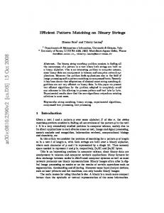
Fig. 1: Algorithm brute-force matrix submatching Main-Matrix

Sub-Matrix

CHAIN CODE BASED METHOD A: 6X6

The matrix submatching or matrix containment problem implies searching for a pattern in the form of a matrix inside a larger matrix. The brute-force algorithm tends to work well for matrices which have no assumptions with respect to their contents. This section introduces another solution for the matrix submatching problem based on chain coding which is a succinct way of representing a list of points[6]. Only a starting point is represented by its location while the other points are represented by successive displacements from point to point along a certain path. For several applications of matrices such as image processing, a matrix tends to have repeating adjacent values representing objects. Although, the proposed solution works for general grey values of elements in matrices, the algorithm will be discussed with respect to binary matrices. Using the

B: 2X2

Fig. 2: Example of main matrix A: 6×6 and submatrix B: 2×2 Chain-code based technique, the process of matrix submatching goes through two phases; namely, transformation and matching. Transformation phase: “chain code matrix transformation” The objective of the transformation phase is to convert the main matrix and submatrix into two sets of vectors with each vector represents the chain code of the elements of the corresponding row in the original matrix. The chain code based transformation takes advantage of repeating values of 79

Am. J. Applied Sci., 6 (1): 78-88, 2008 Row = 1

Row = 1

Row = 1

Row = 1

# of comparisons = 2 # of occurrences = 0 MSM(A,B) = { } Row = 1



# of comparisons = 10 # of occurrences = 1 MSM(A,B)={A(1, 4) } Row = 3

# of comparisons = 11 # of occurrences = 1 MSM = { A(1, 4) } Row = 3




# of comparisons = 24 # of occurrences = 1 MSM = { A(1, 4) }



Row = 4


Row = 5

Row = 5


# of comparisons = 36 # of occurrences = 2 MSM = {A(1, 4), A(4, 5)}

# of comparisons =45 # of occurrences = 2 MSM = {A(1, 4), A(4, 5)}

# of comparisons =46 # of occurrences = 2 MSM = {A(1, 4), A(4, 5)}

Fig. 3: Trace for the brute-force algorithm with respect to matrices A and B in Fig. 2 80

Am. J. Applied Sci., 6 (1): 78-88, 2008

’

// a (i, 1) is the number of the first consecutive zero-value elements in Ai starting with a(i, 1). ’ a (i, 1) 0 if a(i, 1)=1 ’ a (i, 1) r1 if a(i, 1)= a(i, 2)= …= a(i, r1 )=0, where r1 S u b _ co l 2. { m = 1; 3. if (n + 1 > S u b _ ro w ) { 4. n = 1 ; b rea k = tru e; // to b rea k fro m th e w h ile . R etu rn ;} 5. 6. 7. 8. 9.

e lse { n = n + 1 ; if (i + 1 < = M a in _ ro w ) i = i + 1; e lse { sto p = tru e ; b re ak = tru e; // to b rea k fro m th e w h ile. R etu r n ;} } // en d else.

10. 11.

[i, j] = R etu rn o ffse t in T M M () } // en d if.

1 2 . e lse { m = m + 1 ; j = j + 1 ; } 1 3 . R etu r n i, j, n , m ;

Fig. 10: Get the new values of i, j, n, m function A lgorith m : Return offset in T M M () // return th e exact colum n in th e n ext row in T M M to start search in g from . 1. w = 0; sum = 0; 2. wh ile (sum < offset_col) { 3. w = w + 1; 4. sum = sum + T M M ( i, w); } 5. j = w; 6.

if ( T SM (n, m ) = = 0) m = m + 1;

7.

if (m od (j, 2) ~ = 0 & & m od (m , 2) = = 0) {flag = false; break = tr ue; Return ; } // j poin tin g to a on e location , w h ile th e search m ust start fr om a zer o location .

8.

if (m od (j, 2) = = 0 & & m od (m , 2) ~ = 0) {flag = false; break = true; poin tin g to a zero location , wh ile th e search m ust start from a on e location .

9.

[w, x] = Return offset in original M ain M atrix ();

Return ; } // j

10. if (~ (x >= offset_col & & x = TSM (n, m) offset_row = 1 offset_col =(4 - 1)+ 0+1 = 4 i = 1, j = 1, n = 1, m = 1,

TMM (i, j) >= TSM (n, m) offset_row = 1 offset_col = 4 i = 1, j = 2, n = 1, m = 2,

TMM (i, j) >= TSM (n, m) offset_row = 1 offset_col = 4 i = 2, j = 2, n = 2, m = 2.

TMM (i, j) < TSM (n, m) offset_row = 0 offset_col = 0 i = 2, j = 1, n = 1, m = 1,

No. of comparisons: 5

No. of comparisons:6

Match found No. of comparisons:7


TMM (i, j) < TSM (n, m) offset_row = 0 offset_col = 0 i = 3, j = 1, n = 1, m = 1,

TMM (i, j) >= TSM (n, m) offset_row = 3 offset_col = (2 - 1)+ 2+1 = 4 i = 3, j = 3, n = 1, m = 1,





TMM (i, j) >= TSM (n, m) offset_row = 4 offset_col = (2 - 1)+0+1 = 2 i = 4, j = 1, n = 1, m = 1,

TMM (i, j) >= TSM (n, m) offset_row = 4 offset_col = 2 i = 4, j = 2, n = 1, m = 2

TMM (i, j) >= TSM (n, m) offset_row =0 offset_col = 0 i = 5, j = 1, n = 2, m = 2.

In TMM start searching from j = 1, which indicate a location which contains summation of consecutive zero.

85


In TMM start searching from j = 2, incorrect lower boundary. No. ofcomparisons:12

TMM (i, j) >= TSM (n, m) offset_row = 4 offset_col =(1 - 1)+4+1 = 5 i = 4, j = 3, n = 1, m = 1.

Am. J. Applied Sci., 6 (1): 78-88, 2008 No. of comparisons:13




TMM (i, j) >= TSM (n, m) offset_row = 4 offset_col = 5 i = 4, j = 4, n = 1, m = 2,

TMM (i, j) >= TSM (n, m) offset_row = 4 offset_col = 5 i = 5, j = 2, n = 2, m = 2

TMM (i, j) >= TSM (n, m) offset_row =5 offset_col = (4-1)+0+1= 4 i = 5, j = 1, n = 1, m = 1.


Match found No. of comparisons:17


In TMM start searching from j = 3, which indicate a location contains summation of consecutive zero.

Fig. 13: Trace for the chain-code based matrix submatch algorithm for matrices A and B in Fig. 5. occurrences of submatricies in the corresponding main matrices were computed. The outcome of the experiments is summarized in Fig. 14. Our experiments clearly show that the chain code based algorithm requires half the number of comparisons required by the brute-force approach. This is basically attributed to the compression in size due to the preprocessing phase of the chain-code approach. For several applications, it is typical that a database of matrices exists and a query is posed against the database to retrieve all matrices which contain an incoming sub matrix[7, 11]. In such cases, the preprocessing phase for the main matrices needs to be done only once.

RXPERIMENTAL RESULTS The brute-force and chain-code based algorithms are considered sequential search mechanisms for the matrix submatching problem. In order to experimentally compare the performance of both algorithms, we randomly generated a database for main matrices with sizes 50×50, 75×75, 100×100 and 200×200 and another one for submatrices with sizes 10×10, 15×15, 25×25, 30×30, 35×35, 40×40 and 45×45 using Matlab. The databases contain 1000 occurrences of each indicated size and the average numbers of comparisons required by both algorithms to find the 86

Am. J. Applied Sci., 6 (1): 78-88, 2008

Fig. 14: No of Comparisons required by the brute-force and chain-code based Algorithms Table 2: Average percentage of square matrix size (NXN) reduction due to preprocessing phase Percentage of Percentage of Matrix N= size reduction Matrix N= size reduction 2 0 500 49.8 5 30 1,000 49.9 10 40 5000 50.0 15 43.3 10000 50.0 20 45.0 25000 50.0 25 46.0 50000 50.0 50 48.0 100000 50.0 75 48.7 500000 50.0 100 49.0 1000000 50.0

presented in this paper consists of two phases; namely, transformation and matching. The transformation phase reduces the sizes of all relevant matrices by nearly half of their original sizes bringing about clear saving in the number of comparisons when compared with the brute force approach. Although, this paper demonstrated superiority of the chain-code approach for binary square matrices, the results hold true for general matrices.

Table 2 demonstrates the average percentage of size reduction for randomly generated square binary matrices with various sizes. The maximum average percentage of size reduction is 50%.

The authors would like to acknowledge the contribution of Thaer Al-Ibaisi and Khitam Jbara in obtaining experimental results.

ACKNOWLEDGMENT

REFERENCES

CONCLUSION

1.

This article brings focus to the matrix submatching operation as an essential problem to be solved for many applications including watermarking, geographic information systems and pattern recognition. Most of these applications start with a database of matrices and require the retrieval of those matrices which contain an incoming matrix. The chain code based approach

2. 87

Angiulli, F. and E. Cesario, 2006. A Greddy Search Approach to Co-clustering Sparse Binary Matrix, 18th IEEE International Conference on Tools with Artificial Intelligence (ICTAI'06), pp: 363-370. Bronson, R., 1989. Schaum's Outline of Theory and Problems of Matrix Operations, McGraw-Hill.

Am. J. Applied Sci., 6 (1): 78-88, 2008 3.

4.

5.

6.

7.

8.

Koyuturk, M. and A. Grama, 2006. Nonorthogonal decomposition of binary matrices for boundederror data compression and analysis, ACM transactions on mathematical software, 32 (1): 33-69. 9. Robinson, S., 2005. Toward an optimal algorithm for matrix multiplication. SIAM News, 38 (9). 10. Shen, X. and Q. Hu, 1992. Approximate submatrix matching problems. Proceeding of the ACM Symposium on Applied Computing (SAC’92), pp: 993-999. 11. Sleit, A., W. AlMobaideen, A. Baarah and A. Abusitta, 2007. An efficient pattern matching algorithm. J. Applied Sci., 7 (18): 2691-2695. 12. Smith, P., 1991. Experiments with a very fast substring search algorithm. Software-practice and experience. 21 (10): 1065-1074.

Coppersmith, D. and S. Winograd, 1990. Matrix multiplication via arithmetic progressions, J. Symbolic Computat., 9: 251-280. Cormen, T.H., C.E. Leiserson, R.L. Rivest, and C. Stein, 2001. Introduction to Algorithms. 2nd Edn., The MIT Press. Jane, A., 1995. Parallel search with matrices with sorted column, 7th IEEE Symposium on Parallel and Distributed Processing, pp: 224-228. Mei-Chen, Y., Y. Huang and J. Wang, 2002. Scalable Ideal-Segmented Chain Coding, IEEE international conference on image processing. Knuth, D.E., J.H. Morris and V.R. Pratt, 1977. Fast pattern matching in strings, SIAM. J. Comput., 6 (2): 323-350.

88