On Efficient Spatial Matching

On Efficient Spatial Matching Raymond Chi-Wing Wong

Yufei Tao

Ada Wai-Chee Fu

Xiaokui Xiao

Department of Computer Science and Engineering The Chinese University of Hong Kong Sha Tin, New Territories, Hong Kong {cwwong, taoyf, adafu, xkxiao}@cse.cuhk.edu.hk

ABSTRACT This paper proposes and solves a new problem called spatial matching (SPM). Let P and O be two sets of objects in an arbitrary metric space, where object distances are defined according to a norm satisfying the triangle inequality. Each object in O represents a customer, and each object in P indicates a service provider, which has a capacity corresponding to the maximum number of customers that can be supported by the provider. SPM assigns each customer to her/his nearest provider, among all the providers whose capacities have not been exhausted in serving other closer customers. We elaborate the applications where SPM is useful, and develop algorithms that settle this problem with a linear number O(|P | + |O|) of nearest neighbor queries. We verify our theoretical findings with extensive experiments, and show that the proposed solutions outperform alternative methods by a factor of orders of magnitude.

1.

INTRODUCTION

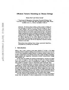
Bichromatic reverse nearest neighbor (BRNN) search is an important operator in spatial databases that has been extensively studied [17, 18, 22, 23, 24]. Specifically, let P and O be two sets of objects in the same data space. Given an object p ∈ P , a BRNN query finds all the objects o ∈ O whose nearest neighbors (NN) in P are p, namely, there does not exist any other object p0 ∈ P such that |o, p0 | < |o, p|. Those objects o constitute the BRNN set of p. A typical application of BRNN retrieval is “selection of the best service”. Consider, for example, that we want to collect voters’ ballots in an election. In Figure 1a, P contains three polling places p1 , p2 , p3 and O includes three residential estates o1 , o2 , o3 . Assume that we want to decide, for each estate oi (1 ≤ i ≤ 3), the polling place that a resident in oi should go to for casting her/his ballot. Naturally, the best polling place is the one closest to oi . By this reasoning, each polling place should be responsible for the estates in its BRNN set. Namely, p1 needs to serve all the estates in O (i.e., the BRNN set of p1 is {o1 , o2 , o3 }), while p2 and p3 serve no estate at all. This assignment of polling-places and estates, unfortunately, fails to account for the fact that each polling place has a “serving capacity”. A reasonable metric for such a capacity, for instance, is the

Permission to copy without fee all or part of this material is granted provided that the copies are not made or distributed for direct commercial advantage, the VLDB copyright notice and the title of the publication and its date appear, and notice is given that copying is by permission of the Very Large Data Base Endowment. To copy otherwise, or to republish, to post on servers or to redistribute to lists, requires a fee and/or special permission from the publisher, ACM. VLDB ‘07, September 23-28, 2007, Vienna, Austria. Copyright 2007 VLDB Endowment, ACM 978-1-59593-649-3/07/09.

p3 o1 o2

p2 o3 (a) Data sets P and O

p1

Estate o1 o2 o3

Population 7k 3k 4k

Poll. place p1 p2 p3

Capacity 10k 10k 10k

(b) Populations and capacities

Figure 1: Inadequacy of BRNN search population of registered voters in all the estates served by the corresponding polling place. Figure 1b demonstrates the population (serving capacity) of each estate (polling place) in Figure 1a. In this case, the assignment determined with BRNN reasoning is not feasible, since the total population in o1 , o2 , and o3 equals 14k, and exceeds the capacity 10k of p1 . Motivated by the above problem, in this paper we study spatial matching (SPM), which can be regarded as a generic version of BRNN search that incorporates serving capacities. Given the data in Figures 1a and 1b, SPM aims at allocating each estate o ∈ O to the polling-place p ∈ P that (i) is as near to o as possible, and (ii) its servicing capacity has not been exhausted in serving other closer estates. These requirements lead to an assignment: {(p1 , o1 ), (p1 , o2 ), (p2 , o3 )}. Note that o3 is served by p2 , instead of its nearest polling place p1 , because the capacity of p1 has been used up in serving o1 and o2 . This arrangement is fair, since it reflects the practical policy that a polling place gives a higher priority to its neighborhood than to a farther area. The rationale of SPM can be understood in two intuitive ways which turn out to be equivalent. First, the SPM-assignment results from repetitively taking the closest pair of polling-place and estate, among all the polling places that can still serve additional estates, and all the estates that have not been allocated. Specifically, at the beginning, (p1 , o1 ) is the closest pair in the cartesian product P × O, and is included in the assignment. Then, o1 is removed from O, after which (p1 , o2 ) becomes the closest pair in the current P × O, and thus, is added to the assignment as well. Next, o2 is eliminated from O. Furthermore, p1 is also excluded from P , since its serving capacity has been exhausted. Now (p2 , o3 ) and (p3 , o3 ) are the only elements in P × O; therefore, (p2 , o3 ) is taken as the last pair in the assignment. Second, interestingly the SPM-assignment is actually the result of a classical problem, called stable marriage [10], between P and O. To understand this, notice that each residential estate o is implicitly associated with a preference list, which sorts the polling places in descending order of how much o would like to be served by them. Similarly, each polling place p also has such a list, which enumerates the estates in descending order of how much p would

like to serve them. Specifically, the preference list of an estate o ∈ O sorts the polling places in P in ascending order of their distances to o. Clearly, all estates in Figure 1a have the same list {p1 , p2 , p3 }. Symmetrically, the preference list of a polling place p ∈ P juxtaposes the estates in ascending order of their distances to p. That is, the list of p1 is {o1 , o2 , o3 }, while those of p2 and p3 are {o3 , o2 , o1 }. Given these lists, stable marriage returns a “fair” assignment, where no polling-place and estate prefer each other to their current matches, respectively. (For example, assignment {(p1 , o3 ), (p2 , o2 ), (p3 , o1 )} is not fair, since p1 and o1 prefer each other more than their existing matches o3 and p3 , respectively.) Although closest pair and stable marriage have been well-studied, existing solutions cannot be applied to solve SPM efficiently. As reviewed in Section 3, the fastest adaptation of those solutions entails O(|P | · |O|) cost in computing an assignment, which is prohibitively expensive for voluminous P and O. In this paper we propose a novel algorithm Chain to enable SPM on large datasets. Chain has provably good asymptotic performance, and terminates after a linear number O(|P |+|O|) of NN (nearest neighbor) queries. This is an important feature, since it opens the opportunity of leveraging the rich literature of NN search to optimize Chain. (For instance, in 2D space, each NN query can be settled in poly-logarithmic time, so that the running time of Chain is O((|P |+|O|)·(log O(1) |P |+ log O(1) |O|)), which significantly improves the best known solution.) Furthermore, Chain is not limited to Euclidean objects and the L2 distance norm. Instead, it is applicable to objects in any metric space, if the adopted distance norm satisfies the triangle inequality. For example, Chain can be leveraged to settle the SPM problem in Figure 1, even if the distance between a polling place and an estate is their road-network distance. The rest of the paper is organized as follows. Section 2 formulates two versions of spatial matching, i.e., un-weighted and weighted SPM, and proves that conventional BRNN search is a special case of our weighted problem. Section 3 clarifies the relations of SPM to existing problems, and explains why the solutions to those problems are not efficient for SPM. Section 4 proposes an algorithm that settles un-weighted SPM, and analyzes its asymptotical performance, whereas Section 5 extends our solution to the weighted version. Section 6 evaluates the proposed techniques through extensive experiments with real data. Section 7 concludes the paper with directions for future work.

2.

BASIC DEFINITIONS AND PROPERTIES

Let D be any metric space, where object distances satisfy the triangle inequality, that is, |a, b| + |b, c| ≥ |a, c| for any objects a, b, c in D. We have a set P of objects in D, each of which represents a service-site (e.g., a polling place in Figure 1a). We also have another set O of objects in the same space, each corresponding to a customer-site (e.g., a residential estate). For each customersite o ∈ O, use o.w to denote its population, i.e., the number of customers in o. Given a service-site p ∈ P , deploy p.w to represent its capacity, equal to the maximum number of customers that can be served by p. We consider that there are enough services for all customers, namely: P P (1) o∈O o.w p∈P p.w ≥ All the definitions, algorithms, lemmas and theorems in this paper apply to any D and distance metric. Nevertheless, to facilitate understanding, our examples are designed in a two-dimensional Euclidean space D, assuming that object distances are measured by the Euclidean norm L2 . In this section, we will first define an un-weighted version of spatial matching, before extending the definitions to the more com-

plicated weighted version. Then, we will discuss a class of nongeographic applications where spatial matching is useful. Finally, several fundamental problem characteristics will be clarified. Un-Weighted Spatial Matching. In the un-weighted version, each customer-site (service-site) has a population (capacity) 1, that is, o.w = 1 and p.w = 1 for any o ∈ O and p ∈ P . D EFINITION 1 (A SSIGNMENT ). Let A be a subset of the cartesian product P × O. Each object-pair in A is a couple, where the two objects are partners to each other. A is called an assignment, if each customer-site o ∈ O appears in exactly one couple, and each service-site p ∈ P appears in at most one couple. We look for a fair assignment which assigns each customer o to its nearest service p, which has not been occupied by any other closer customer. Unfairness is captured by the existence of a “dangling” object pair. D EFINITION 2 (DANGLING PAIR ). Given an assignment A, a pair of objects (p, o) ∈ P × O is a dangling pair if all the following conditions are satisfied: • |p, o| < the distance between o and its partner in A; • |p, o| < the distance between p and its partner in A (this condition is trivially true if p has no partner in A). A is fair, if no dangling pair exists; otherwise, A is unfair. To illustrate this concept, consider that P (O) includes all the cross (dot) points in Figure 1a, and that each customer-/service-site has a population/capacity 1. Then, assignment {(p1 , o1 ), (p2 , o2 ), (p3 , o3 )} is unfair, due to the existence of a dangling pair (p2 , o3 ). In particular, p2 (o3 ) has a partner o2 (p3 ) in the assignment, and (p2 , o3 ) is dangling because |p2 , o3 | < |p2 , o2 | and |p2 , o3 | < |p3 , o3 |. On the other hand, {(p1 , o1 ), (p2 , o3 ), (p3 , o2 )} is fair. P ROBLEM 1. The goal of un-weighted spatial matching (unweighted SPM) is to find a fair assignment. Weighted Spatial Matching. The previous definitions can be directly extended to the general case where service- and customersites have respectively arbitrary capacities and populations, subject to Inequality 1. Specifically, given weighted datasets P and O, we can transform them into un-weighted sets P 0 and O0 as follows. For each service-site p ∈ P (customer-site o ∈ O), we duplicate p.w (o.w) objects at the location of p (o), and add all of them to P 0 (O0 ). Then, the goal of weighted SPM is essentially to discover a fair assignment for the resulting P 0 and O0 . Clearly, this assignment encloses |O 0 | couples. As an example, assume that P (O) involves the cross (dot) points in Figure 1a, whose capacities (populations) are indicated in Figure 1b. By the transformation, P 0 and O0 include 30k and 14k points, respectively. The query result {(p1 , o1 ), (p1 , o2 ), (p2 , o3 )} mentioned in Section 1 can be regarded as an assignment computed from P 0 and O0 that contains 14k couples. For instance, (p1 , o1 ) represents 7k couples, each of which pairs a service-site in P 0 located at p1 with a customer-site in O 0 at o1 . Although the transformation correctly defines weighted SPM, it is cumbersome, since it requires enumeration of a huge number of identical couples. Next, we present an alternative definition based on the same idea as the transformation, but is more concise. That is, we will extend Definitions 1 and 2 to their weighted counterparts.

D EFINITION 3 (W EIGHTED A SSIGNMENT ). Let p be a servicesite in P and o a customer-site in O. A triplet (p, o, w) is an extended couple, where w is an integer, and referred to as the weight of the extended couple. We say that p and o are partners to each other. A weighted assignment A is a set of extended couples, such that • for each customer-site o ∈ O, the sum of the weights of all extended couples in A containing o equals precisely o.w; • for each service-site p ∈ P , the sum of the weights of all extended couples in A containing p does not exceed p.w. Unlike the un-weighted case, each service-site (customer-site) may have multiple partners, because it can appear in several extended couples. To understand this, consider again that P (O) is the cross (dot) datasets in Figure 1a, with capacities (populations) in Figure 1b. A weighted assignment can be {(p1 , o1 , 3k), (p2 , o1 , 4k), (p1 , o2 , 3k), (p1 , o3 , 4k)}. Here, o1 has two partners p1 and p2 , which serve 3k and 4k customers in o1 , respectively. Similarly, p1 has three partners o1 , o2 , and o3 . D EFINITION 4 (DANGLING PAIR ). Given a weighted assignment A, a pair of objects (p, o) ∈ P × O is a dangling pair if all the following conditions are satisfied: • |p, o| < the distance between o and some of its partners in A; • |p, o| < the distance between p and some of its partners in A (this condition is trivially true, if the capacity of p has not been exhausted according to A). A is fair, if no dangling pair exists; otherwise, A is unfair. For instance, in Figure 1, weighted assignment {(p1 , o1 , 3k), (p2 , o1 , 4k), (p1 , o2 , 3k), (p1 , o3 , 4k)} is unfair. Specifically, pair (p1 , o1 ) is dangling because (i) |p1 , o1 | < |p2 , o1 | (note that p2 is a partner of o1 ), and (ii) |p1 , o1 | < |p1 , o2 | (also note that o2 is a partner of p1 ). Weighted assignment {(p1 , o1 , 7k), (p1 , o2 , 3k), (p2 , o3 , 4k)}, on the other hand, is fair. P ROBLEM 2. The goal of weighted spatial matching (weighted SPM) is to find a fair weighted assignment. Applications. SPM can be applied in most (if not all) applications where BRNN search makes sense, and the objective is to guarantee the best service each customer can possibly get, subject to service providers’ capacities, and the priorities of other customers. The notions of “service” and “customer” are general, and can have alternative semantics in different, even non-geographic applications. For example, consider that a computer science department wants to assign a set O of students to a set P of intern jobs. Each job is described by several attributes such as the number of working hours per week, the amount of research work in a scale from 0 (light) to 1 (heavy), the distance from the work location to the university, etc. Each student gives her/his preferences for these attributes. As a result, every job and student can be represented as a multidimensional point (one coordinate per attribute). If we aim at matching, as much as possible, a student’s preferences with a job’s description, allocation of students to jobs is an SPM problem. Here, a “service-site” is a job, and its capacity is the number of vacancies of the job, whereas a “customer-site” is a student, and its population equals 1. The result of SPM ensures that a student gets the best job (minimizing the matching difference), among all jobs that have not been fully occupied by better-matched students.

The above example implies a template for a class of profilematching applications where SPM is particularly useful. Specifically, such an application contains (i) a set P of “items”, whose profiles are represented as points in a multidimensional space, and (ii) a set O of “contenders”, whose preferences are also modeled as points in the same data space. SPM makes sure that each contender obtains the best possible item under a fair competition, adhering to the rule that a pair of contender and item is a better match, if their point representations are closer. Basic Properties. We consider a general situation where each pair of objects in the cartesian product P × O has a distinct distance, namely, for any (p, o) and (p0 , o0 ) in P × O, it holds that |p, o| 6= |p0 , o0 | unless p = p0 and o = o0 . This assumption allows us to avoid several complicated, yet uninteresting, “boundary cases”. Obviously, when the assumption is not fulfilled, we can always apply an infinitesimal perturbation to the positions of some service- or customer-sites, to break the tie of the distances of two object pairs. Due to the tininess of perturbation, query results from the perturbed datasets should be as useful as those from the original datasets. The next two lemmas explain two fundamental facts about SPM. Specifically, Lemma 1 shows that the result of SPM is unique, and Lemma 2 indicates that the conventional BRNN problem is merely a special instance of SPM. L EMMA 1. In un-weighted (weighted) SPM, there is a unique fair (weighted) assignment for any P and O. P ROOF. The proofs of all lemmas and theorems can be found in the appendix. L EMMA 2. Let P and O be two sets of objects in the same metric space. The problem of computing the BRNN set of each object p ∈ P is an instance of weighted SPM, where p.w = |O| for every p ∈ P and o.w = 1 for every o ∈ O.

3. RELEVANCE TO EXISTING PROBLEMS Although SPM has not been studied in the literature, it can be reduced to two known problems: stable marriage and closest-pair retrieval. In Sections 3.1 and 3.2, we will clarify the reduction, and explain the limitation of previous solutions when they are adapted to SPM. Finally, Section 3.3 reviews other work related to SPM. For simplicity, the discussion in this section focuses on un-weighted SPM. However, all the results can be easily extended to the weighted version, which can be transformed to the un-weighted problem, as explained in the previous section.

3.1 Reduction to Stable Marriage Stable marriage is a classical problem in computer science. Let P be a set of men, and O a set of women, such that |P | ≥ |O|. Each man p ∈ P (woman o ∈ O) decides a preference list, which sorts the women (men) in descending order of how much p (o) loves them. Apparently, each man’s (woman’s) preference list has a size |O| (|P |); therefore, all the lists occupy O(|P | · |O|) space. The objective is to find a feasible marriage scheme, where each woman marries a man. The scheme should guarantee the absence of a man p and a woman o, such that p loves o more than his current partner (this is trivially true if p has no partner), and o loves p more than her current partner. As a simple example, consider P = {p1 , p2 } and O = {o1 , o2 }. Assume that p1 and p2 have the same preference list {o1 , o2 }, while the list of o1 is {p1 , p2 }, and that of o2 is {p2 , p1 }. In this case, the marriage scheme {(p1 , o2 ), (p2 , o1 )} is not feasible, since

we can find a man p1 and a woman o1 such that p1 prefers o1 to his current partner o2 , and o1 prefers p1 to her current partner p2 . Given an instance of (un-weighted) SPM, we can construct a stable marriage problem as follows. First, each service-site in P is regarded as a man, and each customer-site in O as a woman. Then, each service-site p decides its preference list, by sorting the customer-sites in O in ascending order of their distances to p. Similarly, the preference list of a customer-site o ∈ O juxtaposes all the service-sites in ascending order of their distances to o. We have:

It is worth mentioning that an “incremental” closest-pair algorithm is developed in [7]. If we define the distance of a pair of objects as their Euclidean distance, the algorithm reports objectpairs in P × O in ascending order of their distances (no worst-case bound, however, is proved for the computation cost). This algorithm cannot be applied for SPM, because it assumes that P and O remain the same during the algorithm’s execution. In our context, an object is removed from both P and O every time a pair of objects is found.

L EMMA 3. A feasible marriage scheme of the constructed stablemarriage problem is a fair assignment for the original un-weighted SPM.

3.3 BRNN and NN Search

The reduction allows us to employ a stable-marriage solution for SPM. The fastest solution is due to Gale and Shapley [10]: it produces a feasible marriage scheme in O(|P | · |O|) time, consuming O(|P | · |O|) space. Furthermore, it is also known that, given arbitrary preference lists, O(|P | · |O|) is indeed the (time and space) lower bound of solving the stable-marriage problem. Fortunately, the lower bound does not apply to SPM. The reason is that SPM is actually a special case of stable marriage, since a preference list in SPM cannot be arbitrary, but instead, must be decided according to the distances between spatial objects. For example, in Figure 1a, in SPM the preference list of p1 must be {o1 , o2 , o3 }. However, if it was a stable marriage problem, p1 could have specified another preference list that permutates the three residential sites in any way. The un-equivalence between stable marriage and SPM is also reflected in the fact that the reverse of the above reduction does not work. In particular, it is not always possible to design two sets P and O of points, whose preference lists (computed as described earlier in the reduction from SPM to stable-marriage) are identical to those of a given stable marriage instance. In Section 4, we will develop an efficient SPM algorithm that entails far less than O(|P | · |O|) cost.

3.2 Reduction to Closest Pair Retrieval Given two sets P and O of objects, a closest pair query finds the pair of objects (p, o) whose distance is the smallest among all object-pairs in the cartesian product P × O. Given an instance of un-weighted SPM with a set P (O) of service- (customer-) sites, we can compute an assignment by repetitively retrieving closest pairs as follows. Initially, the assignment is empty. We first retrieve the closest pair (p, o) from P and O, which is added as a couple to the assignment. Then, we remove p and o from P and O respectively, and repeat the above process, until O becomes empty. At this time, the current assignment becomes final. We have the following result. L EMMA 4. The assignment obtained by repetitive closest-pair retrieval as described earlier is a fair assignment for the original un-weighted SPM. Although the above strategy correctly solves SPM, it incurs expensive cost. Specifically, it requires totally |O| closest pair queries, whereas closest pair retrieval is known to be a costly process in general. In particular, to the best of our knowledge, all the existing closest-pair methods [4, 7, 13, 24] rely on heuristics that do not have good worst-case performance. No asymptotical bound better than the trivial O(|P | · |O|) has been established on the running time (the closest-pair problem is easier when P and O are the same dataset; in that case, the closest-pair can be found in O(|O| log |O|) time [3], if O includes two-dimensional objects). Obviously, leveraging a O(|P | · |O|) closest-pair algorithm to solve SPM results in the terrible running time of O(|P | · |O|2 ).

Bichromatic reverse nearest neighbor (BRNN) search is proposed by Korn and Muthukrishnan [18]. The fastest BRNN algorithm is due to Stanoi et al. [22]. Their solution does not support incremental maintenance of the query result, when the underlying datasets have been updated. To remedy this problem, recently Kang et al. [17] develop an alternative method which continuously captures the result changes, when data updates arrive rapidly in the form of a stream. Xia et al. [23] utilize BRNN search to discover the most “influential” service-site, which has the largest BRNN set. None of the above works, however, can be applied to solve SPM, because, as explained in Lemma 2, BRNN retrieval is only a special case of SPM. It is worth noting that there exists another form of reverse nearest neighbor (RNN) search called monochromatic RNN [18], which has also been extensively studied previously (see [1] and the references therein). Monochromatic RNN involves only a single dataset, and is fundamentally different from SPM. Nearest neighbor (NN) search is among the oldest problems in computational geometry. Given a set S of n two-dimensional data points, any NN query can be solved in O(log n) time, using an index that consumes O(n) space. There exist several indexes that can fulfill this purpose; for example, one obvious solution [8] is to build a trapezoidal map over the Voronoi diagram of S. The problem is harder when updates are allowed on S. Using a randomized technique in [20], each update can be supported in O(log n) cost, and each query is answered in O(log 2 n) time, where n is the size of S at the time of the update/query. Recently, a different tradeoff is presented in [6], where Chan shows that it is possible to achieve O(log n) query cost, but the update time must be increased to O(log 6 n). There has been considerable research that aims at solving NN queries using heuristic-oriented algorithms. Although these algorithms do not have good worst-case asymptotical performance, they have been shown to be fairly efficient in reality. Another important advantage of those algorithms is that, they can be easily extended to support NN retrieval on data of any dimensionality, and can be executed on access methods (e.g., B- and R-trees [2]) available in a commercial database. Among the existing solutions, the branchand-bound [21] and best-first [14] algorithms are the fastest for low-dimensional data, and iDistance [15] is a popular solution in high dimensional spaces. Gowda and Krishna [12] introduce the notion of mutual nearest neighbor. Specifically, two objects p and p0 in the same dataset S are mutual NNs, if p is the NN of p0 in S − {p0 } and p0 is the NN of p in S − {p}. Finding mutual NNs is useful in data mining, and several solutions [5, 9, 11, 12, 16] have been developed. Those solutions all stick to the original definition by Gowda and Krishna, i.e., both mutual NNs come from the same dataset. As clarified shortly, the proposed SPM technique requires a closely relevant concept, but with respect to two datasets.

4. UN-WEIGHTED SPATIAL MATCHING In this section, we settle the un-weighted SPM problem. As will

o1

p1

o2 p2 o4 p 4

o1

p1

o2 p2 o3

o 3p 3

Figure 2: A running example

Figure 3: Illustration of a chain

be elaborated in Section 5, the un-weighted solution can be extended to solve the weighted version. Section 4.1 illustrates several problem characteristics crucial to the proposed algorithm, which is presented in Section 4.2. Section 4.3 analyzes the theoretical performance of our solution.

4.1 Reduction to Bichromatic Mutual NN Search The concept of “mutual nearest neighbor” mentioned in Section 3.3 is “monochromatic”, since it concerns only a single dataset. Next, we define its “bichromatic” counterpart. D EFINITION 5 (B ICHROMATIC M UTUAL NN). An object p ∈ P and an object o ∈ O are bichromatic mutual nearest neighbors, if p is the NN of o in P , and o is the NN of p in O. Since in the sequel all occurrences of “mutual NNs” are bichromatic, we omit the term “bichromatic” for simplicity. Figure 2 shows an example where P = {p1 , p2 , p3 , p4 } and O = {o1 , o2 , o3 , o4 }. Here, (p2 , o2 ), (p3 , o3 ) and (p4 , o4 ) are three pairs of mutual NNs. In general, we have: L EMMA 5. As long as P and O are not empty, there always exists at least a pair of mutual NNs. We observe an important reduction from SPM to bichromatic mutual NN search. L EMMA 6. Let (p, o) ∈ P × O be any pair of mutual NNs. Suppose that we remove p from P , and denote P 0 = P − {p}; similarly, we remove o from O, and denote O 0 = O − {o}. Let A0 be a fair assignment for the SPM with P 0 and O0 . Then, A0 ∪ {(p, o)} is a fair assignment for the SPM with P and O. In Figure 2, as discussed before, (p3 , o3 ) is a pair of mutual NNs. Eliminating p3 and o3 from P and O respectively, we obtain P 0 = {p1 , p2 , p4 } and O0 = {o1 , o2 , o4 }. Notice that A0 = {(p1 , o1 ), (p2 , o2 ), (p4 , o4 )} is a fair assignment for the SPM involving P 0 and O0 . Then, by Lemma 6, we know that A = A0 ∪ {(p3 , o3 )} must be a fair assignment for the original SPM including P and O. Lemma 6 suggests that, after finding a pair (p, o) of mutual NNs in P × O, we can remove p and o from P and O respectively, and then, focus on another SPM problem with smaller datasets P 0 = P − {p} and O 0 = O − {o}. Once a fair assignment A0 has been obtained with respect to P 0 and O0 , we can simply augment A0 with an additional couple (p, o) to obtain a new assignment A, which is guaranteed to be the solution to the original SPM for P and O. Notice that, the same trick can be recursively applied in solving the SPM with P 0 and O0 — discover another pair of mutual NNs, remove them from P 0 and O0 , and then concentrate on the SPM for the remaining data. This idea motivates a neat framework for performing SPM, as is presented in Algorithm 1. E XAMPLE 1. We illustrate Algorithm 1 with the example in Figure 2. At the beginning, we initialize an empty assignment A.

Algorithm 1 General Framework of Spatial Matching (P , O) 1: A ← ∅ 2: while |O| 6= ∅ do 3: find a pair (p, o) of mutual NNs in P and O 4: remove p and o from P and O, respectively 5: A ← A ∪ {(p, o)} 6: return A

Suppose that we find mutual NNs p3 and o3 in the first iteration. Then, (p3 , o3 ) is inserted into A, after which p3 (o3 ) is evicted from P (O), leading to P = {p1 , p2 , p4 } and O = {o1 , o2 , o4 }. Assume that the second iteration retrieves mutual NNs p2 and o2 in the current P and O, respectively. Accordingly, we insert (p2 , o2 ) into A, and eliminate p2 (o2 ) from P (O), leaving P = {p1 , p4 } and O = {o1 , o4 }. The third iteration discovers mutual-NN pair (p4 , o4 ), which is thus added to A. After removing p4 and o4 , P and O become singleton sets {p1 } and {o1 }, respectively. The final iteration thus inserts (p1 , o1 ) into A, which becomes the final assignment for the original SPM problem. Efficient implementation of Algorithm 1 demands a fast solution for fetching a pair of mutual NNs from P and O. As reviewed in Section 3.3, the previous mutual-NN algorithms focus on the monochromatic case, and hence, are inapplicable in our (bichromatic) scenario. An obvious approach to find mutual NNs is to retrieve the closest pair in P × O (using an existing algorithm reviewed in Section 3.2), since the closest pair is definitely a pair of mutual NNs. Unfortunately, this approach degrades Algorithm 1 to precisely the strategy explained in Section 3.2, which entails prohibitive cost. In fact, mutual-NN search is much easier than identifying the closest pair because, intuitively, there exist multiple pairs of mutual NNs (e.g., as mentioned earlier, Figure 2 contains three pairs of mutual NNs), and it suffices to find any of them. In the next subsection, we provide an efficient mutual-NN algorithm.

4.2 The Chain Algorithm Next, we develop an SPM algorithm Chain following the framework in Algorithm 1. Given datasets P and O, Chain retrieves a pair of mutual NNs (from the current P × O), removes them from P and O respectively, and repeats this process. Chain has an important feature: to compute the next mutual-NN pair, it does not start from scratch, but utilizes the information already gathered in finding the previous pair. This feature allows Chain to avoid fetching the same information twice, and guarantees its good asymptotic performance, as studied in the next subsection. The First Mutual-NN Pair. We first explain a method of finding one pair of mutual NNs. The method leverages a chain list C, which contains objects from P and O, and has two invariant properties. First, the elements of C have interleaved origin datasets. That is, if an element is from P , then its successive element must come from O, and vice versa. Second, for any consecutive objects x and y (in this order) in C, y must be the NN of x in the origin dataset of y. C is initially empty. To acquire mutual NNs, we start with an arbitrary object in O, and insert it to C. Then, we carry out a chain process, which repetitively performs the following procedure, until a pair of mutual NNs is discovered. The procedure takes the last element x of the current C. Assuming that x belongs to O (P ), we find the NN y of x in P (O). If y is different from the preceding element of x in C, y is placed at the end of C, and the chain process continues with another execution of the above procedure. Otherwise, we have identified the first pair of mutual NNs x and y.

The above strategy guarantees the retrieval of a mutual-NN pair, due to the following observation: L EMMA 7. Each object in P or O appears in C at most once. In other words, C cannot keep expanding forever, since both P and O have a limited cardinality. In fact, usually mutual NNs can be found after only a small number of NN queries. This can be well illustrated using Figure 3, where P = {p1 , p2 } and O = {o1 , o2 , o3 }. Here, o1 is a random point from O, and the first element of C. Then, we fetch the NN p1 of o1 in P , and append it to C (= {o1 , p1 } currently). Likewise, the NN of p1 in O is point o2 . Since o2 is different from o1 (the preceding element of p1 in C), o2 is also appended to C. Similarly, next p2 is included in C, followed by o3 , at which point the content of C is {o1 , p1 , o2 , p2 , o3 }. Now we retrieve the NN of o3 in P , which turns out to its preceding element p2 . Hence, a mutual-NN pair (p2 , o3 ) is found. Let us draw a circle centering at each element in C that crosses its NN in the opposite dataset. For example, the circle at o1 crosses p1 , whose circle passes o2 , etc. The sizes of the circles decrease monotonically, as we traverse their centers according to their ordering in C. (This observation is easy to prove. For instance, the circle at p1 cannot cover o1 , because |p1 , o2 | < |p1 , o1 | due to the fact that o2 is the NN of p1 in O; therefore, the circle at p1 is smaller than that at o1 .) The implication is that, assuming the last element x of C belongs to O (P ), C expands, only if there is an unseen point in P (O) whose distance to x is smaller than the radius of the circle centering at the preceding element of x. Such a point x cannot be found, after the radius becomes sufficiently small — this is when a mutual-NN pair is identified. The Next Pair. Consider the moment of encountering a pair of mutual NNs. Without loss of generality, assume that at this time the last element of C originates from P (the opposite case is similar). Let us represent the content of C as {o1 , p1 , ..., om , pm }, where m is some positive integer, and for any i ∈ [1, m], oi ∈ O and pi ∈ P . Here, om and pm are mutual NNs. We now update P (O) by deleting pm (om ), and then proceed to look for the next mutual-NN pair. Although this can be achieved trivially by applying the procedure of obtaining the first pair, a much better approach would be to utilize the current content of C, if C is not empty. Specifically, after pm and om are removed from C, the remaining elements still satisfy the two invariant properties stated earlier, with respect to the updated P and O. That is, for any consecutive elements x and y of C (in this order), (i) they are from different datasets, and (ii) y is the NN of x in the origin dataset of y. Therefore, it is not necessary to grow C from the beginning; instead, we can continue the chain process from the current last element of C. Formal Algorithm and Illustration. The previous discussion has elaborated the details of Chain, as presented in Algorithm 2. In the sequel, we illustrate the algorithm using a concrete example. E XAMPLE 2. Consider that we want to find the fair assignment for the SPM problem involving the data in Figure 2, where P = {p1 , p2 , p3 , p4 } and O = {o1 , o2 , o3 , o4 }. Chain starts by initiating an empty A and C, choosing a random element o1 from O, and inserting it to C. Then, it finds the NN p1 of o1 in P , after which C = {o1 , p1 }. Next, the NN o2 of p1 in O is retrieved. Since o2 is different from o1 (the preceding element of p1 ), C is expanded to {o1 , p1 , o2 }. Chain proceeds by fetching the NN p2 of o2 in P , and appending p2 to C. The algorithm then searches for the NN of p2 in O, which coincides with the preceding element o2 of p2 in C. Hence, a pair (p2 , o2 ) of mutual NNs is discovered. Figure 4a illustrates the current chain.

Algorithm 2 Chain (P , O) 1: A ← ∅ 2: while O 6= ∅ do 3: pick a random object o ∈ O 4: C ← {o} 5: while C 6= ∅ do 6: x ← the last element of C 7: if x ∈ O then 8: y ← the NN of x in P 9: if y = the previous element of x in C then 10: remove y and x from C 11: insert (y, x) into A 12: remove y and x from P and O, respectively 13: else 14: insert y into C 15: else 16: y ← the NN of x in O 17: if y = the previous element of x in C then 18: remove y and x from C 19: insert (x, y) into A 20: remove x and y from P and O, respectively 21: else 22: insert y into C 23: return A

According to the analysis in Section 4.1, (p2 , o2 ) must be a couple in our objective assignment, and hence, is inserted in A. After this, p2 and o2 are evicted from C (which becomes {o1 , p1 }), and then further eliminated from P and O, respectively (now P = {p1 , p3 , p4 } and O = {o1 , o3 , o4 }). Since p1 is the last element of C, Chain continues by searching for the NN of p1 in O, and retrieves o4 , which is appended to C. Next, the algorithm fetches the NN p4 of o4 in P , updates C to = {o1 , p1 , o4 , p4 }, and then (through an NN query triggered by p4 ) discovers that p4 and o4 are mutual NNs. Figure 4b demonstrates the chain at this moment. After adding (p4 , o4 ) to A, we remove p4 (o4 ) from P (O) and C. p1 becomes the last element of C, and its NN in O is o1 , which precedes p1 in C. So, Chain acquires the third mutual-NN pair (p1 , o1 ), which is included in A. Figure 4c presents the current chain. Continuing the example, we delete p4 and o4 from C, and from P and O, respectively. Now C becomes empty. Hence, Chain picks another random point from O, and settles on o3 , since it is the only point left in O. Finally, (p3 , o3 ) is produced as the last pair of mutual NNs, and enters A. The algorithm terminates with the fair assignment A = {(p1 , o1 ), (p2 , o2 ), (p3 , o3 ), (p4 , o4 )}. We index P and O with a multidimensional access method efficient for NN search. If such an index does not exist in advance, it is constructed (through a bulkloading algorithm [19], whenever possible) before the execution of Chain. Obviously, the index needs to be dynamic, namely, it must allow incremental object deletions.

4.3 Analysis The cost of Chain is dominated by the overhead of two operations: NN search, and deletion of an object (from P or O). We first bound the numbers of these operations, respectively: T HEOREM 1. Chain performs at most 3|O| NN queries, and exactly 2|O| object deletions. In other words, the number of operations of each type is linear to the cardinality of dataset O. The efficiency of each operation depends on the data structure used to index O and P . Without being limited to any specific structure, let us use α(n) (β(n)) as the

o1

p1

o2 p2 o4 p 4

o1

p1

o 3p 3

(a) When (p2 , o2 ) is found

o4 p 4

o 3p 3

(b) When (p4 , o4 ) is found

o1

p1 o 3p 3

(c) When (p1 , o1 ) is found

Figure 4: Illustration of chains in solving the SPM problem in Figure 2 worst-case asymptotical complexity of an NN query (object deletion) performed on the structure, when the underlying dataset has a cardinality n. Then, a general result holds: T HEOREM 2. The running time of Chain is O(|O| · (α(|P |) + β(|P |))). For example, as mentioned in Section 3.3, if the technique of [20] is deployed to manage two-dimensional O and P , α(|P |) = log 2 (|P |) and β(|P |) = log(|P |), whereas if the solution of [6] is utilized, α(|P |) = log(|P |) and β(|P |) = log 6 (|P |). In either case, the overall time complexity of Chain is O(|O| · log O(1) |P |).

5.

WEIGHTED SPATIAL MATCHING

In Section 5.1, we extend Chain (Algorithm 2) to solve the weighted SPM problem, where o.w ≥ 1 and p.w ≥ 1 for all o ∈ O and p ∈ P . Then, Section 5.2 analyzes the performance of the extended algorithm.

5.1 The Weighted Chain Algorithm Algorithm 3 presents the proposed solution Weighted-Chain for settling weighted SPM. As with Chain, Weighted-Chain works by continuously retrieving mutual NNs. The difference between the two algorithms lies in how a mutual-NN pair is handled. In particular, Weighted-Chain generates extended couples (see Definition 3) from a pair of mutual-NNs, after which usually only one object in the pair is removed from its origin dataset (as opposed to always eliminating both objects in Chain). Let us elaborate the details of Weighted-Chain. It maintains a variable A which stores the extended couples already discovered, and becomes the final weighted assignment at the end of the algorithm. Initially, A is ∅. We start by randomly selecting an object o ∈ O, and initialize the chain list C to {o}. Then, as long as C is not empty, Weighted-Chain carries out the following procedure repetitively. Take the last element x of C, and without loss of generality, assume that x comes from O (the scenario where x ∈ P is symmetric). We fetch the NN y of x in P , and then distinguish two cases. 1. If y is not the preceding element of x in C, we simply insert y into C. 2. Otherwise, a pair of mutual NNs y, x has been identified. Thus, we generate an extended couple as follows, depending on the comparison of x.w and y.w. (a) If x.w > y.w, we insert (y, x, y.w) into A. Furthermore, both x.w and y.w are reduced by y.w (i.e., y.w equals 0 afterwards), We remove y from P and C, and x from C. (b) If x.w ≤ y.w, we add (y, x, x.w) to A. Both x.w and y.w are decreased by x.w. After this, x is removed from O and C. If y.w equals 0 (which happens only if x.w = y.w), we also discard y from P and C. Next we illustrate the algorithm with a concrete example.

Algorithm 3 Weighted Chain (P , O) 1: A ← ∅ 2: while O 6= ∅ do 3: pick a random object o ∈ O 4: C ← {o} 5: while C 6= ∅ do 6: x ← the last element of C 7: if x ∈ O then 8: y ← the NN of x in P 9: if y is equal to the previous element of x in C then 10: if x.w > y.w then 11: insert (y, x, y.w) into A 12: decrease x.w by y.w 13: remove y from P 14: remove x and y from C 15: else 16: insert (y, x, x.w) into A 17: decrease y.w by x.w 18: remove x from O and C 19: if y.w = 0 then 20: remove y from P and C 21: else 22: insert y into C 23: else 24: /* Case: x ∈ P . Details omitted, as they are symmetric to the case of x ∈ O.*/

25: return A

E XAMPLE 3. Consider the weighted SPM problem involving the data in Figure 5a where P = {p1 , p2 , p3 } and O = {o1 , o2 , o3 }, and their populations/capacities are as indicated in the figure. Initially, A is ∅. Suppose that Weighted-Chain randomly selects o1 . Then, it performs a sequence of NN queries (in the same way as Chain) until the first pair of mutual NNs p1 and o2 is found. At this point, C = {o1 , p1 , o2 }, and the chain is demonstrated in Figure 5b. As p1 .w = 20 > o2 .w = 10, we create an extended couple (p1 , o2 , 10), and insert it in A. Both p1 .w and o2 .w are reduced by 10, after which p1 .w = 10 and o2 .w = 0. Semantically, the reduction implies that all the customers at o2 have been served, whereas the service-site p1 can still serve 10 more customers. We remove o2 from O and C, which changes to {o1 , p1 }. On the other hand, p1 remains in P and C because, as mentioned earlier, its serving capacity has not been exhausted yet. Next, Weighted-Chain proceeds with additional NN queries to find the second pair of mutual NNs p1 and o3 , at which moment C = {o1 , p1 , o3 } and the chain is shown in Figure 5c (notice that, compared to Figure 5b, o2 has disappeared and p1 .w has changed). Since o3 .w = 15 > p1 .w = 10, an extended couple (p1 , o3 , 10) is added to A. Now we decrease o3 .w and p1 .w by 10, leaving o3 .w = 5 and p1 .w = 0. This time, service-site p1 can serve no more customer; hence, it is eliminated from P and C. Customersite o3 is kept in O, as some customers in o3 are not served yet. However, o3 must be evicted from C (which equals {o1 } after the eviction), because otherwise, o1 and o3 would come together in C, which is not allowed since each pair of consecutive elements in C are required to originate from different datasets. Similarly, the next mutual NNs retrieved are p2 and o1 , with

p2

p1

o1

o2 p3

o3

10 10 15

P p1 p2 p3

20 10 10

(a) Datasets P and O

p2

p1

o1

o3

p3

w

O o1 o2 o3

p2

w p1

o1

10 0 15

P p1 p2 p3

10 10 10

p3

o3

10 10 15

P p1 p2 p3

20 10 10

w

(b) Chain at the moment of finding (mutual NNs) p1 , o2

w

O o1 o2 o3

o2

w

O o1 o2 o3

O o1 o2 o3

p2

w o1

(c) At finding p1 , o3

o3

p3

P p1 p2 p3

w 10 0 5 w 0 10 10

(d) At finding p2 , o1

o3

p3

O o1 o2 o3

w

P p1 p2 p3

w

0 0 5

0 0 10

(e) At finding p3 , o3

Figure 5: Illustration of Algorithm Weighted-Chain C = {o1 , p2 } and the chain illustrated in Figure 5d. Here, p2 .w = o1 .w = 10. Accordingly, we augment A with an extended couple (p2 , o1 , 10), and reduce p2 .w and o1 .w by 10, which become 0. Hence, both o1 and p2 are discarded from C, and their origin datasets O and P , respectively. As C is empty now, Weighted-Chain starts a new chain by randomly choosing another point o3 in O (in fact, o3 is the only object left in O). Finally, an extended couple (p3 , o3 , 5) is inserted into A (see Figure 5e for the current chain), and o3 is deleted from O. As O becomes ∅, Algorithm 3 terminates, returning the final weighted assignment A = {(p1 , o2 , 10), (p1 , o3 , 10), (p2 , o1 , 10), (p3 , o3 , 5)}.

5.2 Analysis Since the correctness of Weighted-Chain is less trivial (than that of Chain), we prove it in the next lemma. L EMMA 8. Algorithm 3 returns a fair weighted assignment. As with Chain, the efficiency of Weighted-Chain is decided by the numbers of NN queries and object deletions, both of which are bounded by O(|P | + |O|), as formalized in: T HEOREM 3. Weighted-Chain performs at most 3(|P | + |O|) NN queries, and at most |P | + |O| object deletions. Again, let us introduce α(n) and β(n) as the worst-case complexities of an NN query and an object deletion respectively, performed on an index used to organize P and O, when the underlying dataset has a size n. We have the following. T HEOREM 4. The running time of Weighted-Chain is O((|P |+ |O|) · (α(|P |) + β(|P |) + α(|O|) + β(|O|))). With the same choices for the index as stated in Section 4.3, the time of Weighted-Chain is bounded by O((|P |+|O|)·(log O(1) |P |+ log O(1) |O|)).

Dataset CA LB GR GM

Dim. 2 2 2 2

Cardinality 62,556 53,145 23,268 36,334

Table 1: Summary of the real datasets

Dim. Cardinality (|O|) Cardinality (|P |)

Default value 1 3 5k 2|O|

Default value 2 3 50k 2|O|

Table 2: Default values of synthetic datasets

6. EMPIRICAL STUDY We have conducted extensive experiments on a Pentium IV 2.2GHz PC with 1GB memory, on a Linux platform. The algorithms were implemented in C/C++. We deployed four real datasets which are available at http://www.rtreeportal.org/spatial.html. The summary of the real datasets is shown in Table 1. Specifically, CA, LB, GR and GM contain 2D points representing geometric locations in California, Long Beach Country, Greece and Germany, respectively. For datasets containing rectangles, we transformed them into points by taking the centroid of each rectangle. For all datasets, each dimension of the data space is normalized to range [0, 10000]. Since SPM involves two datasets, namely P and O, we generated four sets of experiments for real datasets, namely CA-GR, LB-GR, CA-GM and LB-GM , representing (P, O) = (CA, GR), (LB, GR), (CA, GM ) and (LB, GM ), respectively. We also created synthetic datasets each of which contains P following Gaussian distribution and O following Zipfian distribution. The coordinates of each point were generated in the range [0, 10000]. In P , each coordinate follows Gaussian distribution where the mean and the standard derivation are set to 5000 and 2500. In O, each coordinate follows Zipfian distribution skewed towards 0 where the skew coefficient is set to 0.8. In both cases, all coordinates of each point were generated independently. Each data point in both real datasets and synthetic datasets has population/capacity equal to 1 implicitly. These datasets are regarded as the datasets for un-weighted SPM. For weighted SPM, we generated the population/capacity of each data point in these datasets according to the distribution of its neighborhood. We assigned a higher population/capacity if the density of its neighborhood is greater. For each data point p, we performed a range query with radius r from p and obtained the number of data points in this range query, say k. p.w was generated according to a Gaussian distribution where mean is set to k and the standard deviation is

set to 10. In all experiments, we set r to 5% of the range of the dimension. We denote our proposed algorithm as Unweighted Chain and Weighted Chain for unweighted SPM and weighted SPM. We simply denote it as Chain if the context is clear. We compare our proposed algorithm with two adapted solutions to our problem, namely Gale-Shapley and Closest Pair. Gale-Shapley algorithm [10] is the best-known algorithm for the stable marriage problem. We adopt [7] as the closest pair algorithm which finds the solution by repetitive closest-pair retrieval. The implementations of Gale-Shapley and Closest Pair are straightforward in un-weighted SPM problem. Note that, in weighted SPM problem, for the sake of fairness of comparison, we implemented Gale-Shapley and Closest Pair in a way similar to Weighted Chain, instead of transforming the data points as described in Section 2. In Chain and Closest Pair algorithms, we adopted an R*-tree [2] as an indexing structure for the nearest neighbor search where the node size is fixed to 1k bytes 1 . The maximum number of entries in a node is equal to 50, 36, 28 and 23 for dimensionality equal to 2, 3, 4 and 5, respectively. We set the minimum number of entries in a node to be equal to half of the maximum number of entries. We evaluated the algorithms in terms of three measurements: preprocessing time, execution time and memory usage. Since both Chain and Closest Pair require to build indexings for P and O, the preprocessing time of these two algorithms is equal to the time of building the indexings. The preprocessing time of Gale-Shapley is equal to the time of constructing the preference lists of P and O from the data. The execution time corresponds to the time of executing the algorithms. The memory usage of Chain and Closest Pair is equal to the memory occupied by the indexings. The memory usage of Gale-Shapley is equal to the size of the preference lists. Besides, we also evaluated Chain with the ratio of the total number of NN queries in order to verify our theoretical claims in Theorem 1 and Theorem 3. In un-weighted SPM, we report the total number of NN queries divided by |O|. In weighted SPM, we report the total number of NN queries divided by (|P | + |O|). In the experiments, we will study the effect of cardinality, dimensionality and the real datasets for both un-weighted SPM problem and weighted SPM problem. Besides, all experiments were conducted 100 times and we took the average for the results. We present our results into two parts. The first part, Section 6.1, focuses on the performance comparison among all algorithms. Since Gale-Shapley and Closest Pair are not scalable to large datasets, we compare them in Section 6.1. The second part, Section 6.2, focuses on the scalability of our proposed algorithm on datasets with larger cardinality.

6.1 Comparisons We compare the algorithms with real datasets and synthetic datasets. The default values of the synthetic datasets are shown in Table 2. The default value 1 and the default value 2 are the sets of default values used in this section and Section 6.2, respectively. The default values of the real datasets are also same as the default value 1 in Table 2 except the dimensionality where the dimensionality of the real datasets equals 2. Since these values are smaller than the cardinality of the real datasets, we sample the data points accordingly. Effect of Cardinality: In Figure 6, we varied the cardinality |O| of the datasets from 1k to 5k where |P | = 2|O| for un-weighted SPM problem. In Figure 6a, the preprocessing time of Gale-Shapley is 1 We choose a smaller page size to simulate practical scenarios where the dataset cardinality is much larger.

largest since it has to compute all pairwise distances in order to construct the preference lists. The preprocessing times of Chain and Closest Pair are similar because both involves the same preprocessing step of constructing the indexings. It is trivial that the preprocessing time of all algorithms increases with cardinality. The execution times of Chain and Closest Pair is the shortest and the longest, respectively, as shown in Figure 6b. As we analyzed in Section 3, Closest Pair performs the worst and Gale-Shapley is the second worst. In particular, the execution times of Chain, GaleShapley and Closest Pair are 3.39s, 24.81s and 514.06s, respectively, on average when the cardinality (|O|) is equal to 5k. Chain performs 7.32 times faster than Gale-Shapley and 151.64 times faster than Closest Pair. The execution time of all algorithms increases with cardinality. Since Gale-Shapley requires the preference lists which takes O(|P | · |O|), the memory usage is extremely larger than those of Chain and Closest Pair requiring indexings which are typically smaller than O(|P | · |O|). The memory usage is shown in Figure 6c. We also measure the total number of NN queries issued by Chain. This number divided by |O| is shown in Figure 6d. This figure verifies the theoretical claim as shown in Theorem 1 where the ratio is at most 3. Since the cardinality does not have significant effect on this number, the number remains nearly unchanged when cardinality increases. We have also conducted a similar set of experiments for weighted SPM problem with the datasets with populations/weights associated to each data point. We used the same sets of data but generated the populations/weights to each data point as described previously in this section. The results are also similar to un-weighted SPM problem, as shown in Figure 7. The preprocessing time and the memory usage of all algorithms are nearly the same as the unweighted SPM problem, as shown in Figures 7a and c. However, in Figure 7b, the execution time of all algorithms is larger compared with un-weighted SPM problem. For example, when the cardinality equals 5k, the execution times of Chain, Gale-Shapley and Closest Pair for weighted SPM problem are equal to 6.66s, 56.61s and 1,118.98s, respectively. Chain performs 8.5 times and 168.02 times faster than Gale-Shapley and Closest Pair, respectively. Compared with un-weighted SPM problem, the execution time of all algorithms are about two times slower. Figure 7d shows the number of NN queries divided by (|P | + |O|). We also find that the ratio is at most 3, which is consistent with our theoretical result in Theorem 3. In the rest of this section, we only show the results of weighted SPM problem for the sake of space since the results from un-weighted SPM problem and weighted SPM problem are similar. Effect of Dimensionality: Figure 8a shows that the dimensionality does not have significant effect to any algorithm. Gale-Shapley increases slightly with the dimensionality because the preprocessing step requires computations of pairwise distances and the computation time depends on the dimensionality. Both Chain and Closest Pair remain nearly the same when dimensionality increases since the dimensionality does not affect the construction time of indexings too much. However, in Figure 8b, both Chain and Closest Pair increase with dimensionality because both algorithms require real-time computations of distances which depends on dimensionality. However, Gale-Shapley remains nearly unchanged because it depends on the preference lists during execution where the preference lists are already built and do not depend on the dimensionality. Figure 8c shows that the dimensionality does not affect the memory usage of any algorithms significantly. Similarly, we verify our theoretical results as shown in Figure 8d. Effect of Real Datasets: We conducted experiments on the four sets of real datasets, namely CA-GR, LB-GR, CA-GM and LB-

GM . The results are also similar to synthetic datasets. Besides, for the sake of space, we omit the figures. Consider CA-GR. The execution times of Chain, Gale-Shapley and Closest Pair are 5.32s, 160.00s and 415.20s, respectively, on average. Our proposed algorithm have 30.08 times and 78.05 times faster execution time than Gale-Shapley and Closest Pair, respectively. Besides, the memory usage of Chain and Closest Pair is about 3.48MB but the memory usage required by Gale-Shapley is 400MB.

6.2 Scalability We study the scalability of Chain for both un-weighted SPM problem and weighted SPM problem in this section. The default values of the synthetic datasets are the default value 2 shown in Table 2. In these experiments, we do not sample the real datasets. Instead, the cardinality and the dimensionality of the real datasets used in the experiments are shown in Table 1. Figure 9, Figure 10 and Figure 11 show the results when we vary cardinality, dimensionality and different sets of real datasets, respectively. We show Unweighted Chain and Weighted Chain in the figures for un-weighted SPM problem and weighted SPM problem, respectively. Similarly, Unweighted Chain and Weighted Chain have similar preprocessing time and similar memory usage. Besides, the difference in the execution times between Unweighted Chain and Weighted Chain is larger when cardinality and dimensionality is larger. The total number of NN queries obtained here also matches our theoretical results. Conclusion: In conclusion, we find that our proposed algorithm performs the fastest among the tested algorithms in terms of the preprocessing time and the execution time. Besides, it utilizes the lowest memory cost during execution. Our proposed algorithm is scalable to large dataset but Gale-Shapley and Closest Pair are not.

7.

CONCLUSIONS AND FUTURE WORK

This paper proposes a new operator called spatial matching (SPM), which is useful to a large number of profile-matching applications. SPM guarantees the best service for every customer, taking into account the preferences of all customers and service providers. We carry out a systematic study of SPM. First, we carefully formalize two versions, un-weighted and weighted, of the problem. Second, we analyze the connections between SPM and several existing problems (particularly, stable marriage and closest-pair retrieval), and show that the adapted solutions of those problems incur expensive overhead in SPM. Finally, we develop efficient algorithms with good theoretical performance guarantees, and verify their practical efficiency with extensive experiments. This work also opens several directions to future research. First, in this paper we consider that both participating datasets P and O are static. When they are dynamic, i.e., new (existing) customer/service-sites may be inserted (deleted), the result of SPM may also change. How to incrementally maintain the SPM result (without invoking the algorithms developed in this paper) is a promising problem. Second, our solutions assume that each customer can be assigned to any service, while in general a customer o may specify several services that o would like to avoid. For example, in the intern job allocation application mentioned in Section 2, each student (i.e., a customer) may name a few jobs (services) that s/he is not willing to take. It is interesting to investigate how to incorporate such “avoidance-lists” in SPM. ACKNOWLEDGEMENTS: This research was supported by the RGC Earmarked Research Grant of HKSAR CUHK 4120/05E and 1202/06.

REFERENCES [1] E. Achtert, C. Bohm, P. Kroger, P. Kunath, A. Pryakhin, and M. Renz. Efficient reverse k-nearest neighbor search in arbitrary metric spaces. In SIGMOD, 2006. [2] N. Beckmann, H.-P. Kriegel, R. Schneider, and B. Seeger. The R*-tree: An efficient and robust access method for points and rectangles. In SIGMOD, 1990. [3] J. L. Bentley and M. I. Shamos. Divide-and-conquer in multidimensional spaces. In STOC, 1976. [4] C. Bohm and F. Krebs. High performance data mining using the nearest neighbor join. In ICDM, 2002. [5] M. Brito, E. Chaves, A. Quiroz, and J. Yukich. Connectivity of the mutual k-nearest-neighbor graph in clustering and outlier detection. In Statistics and Probability Letters, 1997. [6] T. M. Chan. A dynamic data structure for 3-d convex hulls and 2-d nearest neighbor queries. In SODA, 2006. [7] A. Corral, Y. Manolopoulos, Y. Theodoridis, and M. Vassilakopoulos. Closest pair queries in spatial databases. In SIGMOD, 2000. [8] M. de Berg, M. van Kreveld, M. Overmars, and O. Schwarzkopf. Computational Geometry: Algorithms and Applications. Springer, 2000. [9] C. Ding and X. He. K-nearest-neighbor consistency in data clustering: Incorporating local information into global optimization. In SAC, 2004. [10] D. Gale and L. Shapley. College admissions and the stability of marriage. In Amer. Math. Monthly, 69(1962) 9-15, 1962. [11] K. Gowda and G. Krishna. Agglomerative clustering using the concept of mutual nearest neighbor. In Pattern Recognition, 1978. [12] K. Gowda and G. Krishna. The condensed nearest neighbor rule using the concept of mutual nearest neighborhood. In IEEE Trans. on Info. Theory, 1979. [13] G. R. Hjaltason and H. Samet. Incremental distance join algorithms for spatial databases. In SIGMOD, 1998. [14] G. R. Hjaltason and H. Samet. Distance browsing in spatial databases. TODS, 24(2):265–318, 1999. [15] H. V. Jagadish, B. C. Ooi, K.-L. Tan, C. Yu, and R. Z. 0003. iDistance: An adaptive B+-tree based indexing method for nearest neighbor search. TODS, 30(2):364–397, 2005. [16] W. Jin, A. K. H. Tung, J. Han, and W. Wang. Ranking outliers using symmetric neighborhood relationship. In PAKDD, 2006. [17] J. M. Kang, M. F. Mokbel, S. Shekhar, T. Xia, and D. Zhang. Continuous evaluation of monochromatic and bichromatic reverse nearest neighbors. In ICDE, 2007. [18] F. Korn and S. Muthukrishnan. Influence sets based on reverse nearest neighbor queries. In SIGMOD, 2000. [19] S. T. Leutenegger, J. M. Edgington, and M. A. Lopez. Str: A simple and efficient algorithm for r-tree packing. In ICDE, 1997. [20] K. Mulmuley. Computational Geometry: An Introduction Through Randomized Algorithms. Prentice Hall, 1993. [21] N. Roussopoulos, S. Kelley, and F. Vincent. Nearest neighbor queries. In SIGMOD, 1995. [22] I. Stanoi, M. Riedewald, D. Agrawal, and A. E. Abbadi. Discovery of influence sets in frequently updated databases. In VLDB, 2001. [23] T. Xia, D. Zhang, E. Kanoulas, and Y. Du. On computing top-t most influential spatial sites. In VLDB, 2005. [24] C. Yang and K.-I. Lin. An index structure for improving nearest closest pairs and related join queries in spatial databases. In IDEAS, 2002.

APPENDIX P ROOF OF L EMMA 1: We prove by contradiction. Suppose there exist two different fair assignments, namely A1 and A2 . We want to consider the differences between A1 and A2 . Let Ac = A1 ∩ A2 . Let A01 = A1 − Ac and A02 = A2 − Ac . Since A01 and A02 are of same cardinalities (= |O|), we know that both A01 and A02 are non-empty. Otherwise, A1 and A2 are equal. Let B = A01 ∪ A02 . If (p, o) ∈ A (where A is an assignment), we say that (p, o) is an edge in the following. Consider the edge (p, o) in B with the smallest distance |p, o|. Without loss of generality, we assume that (p, o) ∈ A01 . Since each o ∈ O has exactly one partner and each p ∈ P has at most one partner in both A1 and A2 , there exists at least one and at most two adjacent edges to (p, o) in B. We consider two cases: Case 1: There exist two adjacent edges to (p, o) in B, say (p0 , o) (connecting at o) and (p, o0 ) (connecting at p). We know that (p0 , o) ∈ A02 and (p, o0 ) ∈ A02 . Note that, for any p, p00 ∈ P and o, o00 ∈ O, we have |p, o| 6= |p00 , o00 | unless p = p00 and o = o00 . Besides, since |p, o| is the smallest in B, we have |p0 , o| > |p, o|. Similarly, we also obtain |p, o0 | > |p, o|. We conclude that (p, o) is

30 20 10

10

1

Total no. of NN queries/|O|

40

Chain Gale-Shapley Closest Pair

100

Memory usage (MB)

Execution time (s)

Preprocessing time (s)


50


100

10

1

0 1

2

3

4

5

1

2

Cardinality (in thousands)

3

4

5

1


2

3

4

Chain

4 3.5 3 2.5 2 1.5 1 0.5 0

5

1

2


3

4

5


30 20 10

Memory usage (MB)

40


100

10


100

10

1

1 0 1

2 3 4 Cardinality (in thousands)

5

1


5

1


5

Total no. of NN queries/(|P|+|O|)

1000


50

Execution time (s)


(a) (b) (c) (d) Figure 6: Effect of cardinality for un-weighted SPM problem (synthetic dataset where dimensionality = 3) Chain

2.5 2 1.5 1 0.5 0 1

2 3 4 5 Cardinality (in thousands)

40 30 20 10


1000

Memory usage (MB)


50

Execution time (s)


60

100

10

Chain Gale-Shapley Closest Pair 100

10

0 2

3 4 Dimensionality

5

2

3 4 Dimensionality

5

2

3 4 Dimensionality

5

Total no. of NN queries/(|P|+|O|)

(a) (b) (c) (d) Figure 7: Effect of cardinality for weighted SPM problem (synthetic dataset where dimensionality = 3) Chain

2.5 2 1.5 1 0.5 0 2

3 4 Dimensionality

5

800 600 400 200 0

0

20

40

60

80

100

50 40 30 20 10 0

0


20

40

60

80

100

0


20

40

60

Unweighted Chain Weighted Chain

4


60

80

4

3.5

3.5

3

3

2.5

2.5

2

2

1.5

1.5

1

1

0.5

0.5

0

100

0 10


Total no. of NN queries/(|P|+|O|) (Weighted Chain)

70


1000

Total no. of NN queries/|O| (Unweighted Chain)


Memory usage (MB)

180 160 140 120 100 80 60 40 20 0

Execution time (s)


(a) (b) (c) (d) Figure 8: Effect of dimensionality for weighted SPM problem (synthetic dataset where cardinality (|O|) = 5k)

30

50

70

90


80 60 40

1200 1000 800 600 400

20

200

0

0 3

4

5

2

Dimensionality

3

4

5

2

Dimensionality

3

4


4


40 35 30 25 20 15 10 5 0

4

3.5

3.5

3

3

2.5

2.5

2

2

1.5

1.5

1

1

0.5

0.5

0

5

0 2

Dimensionality


100

2


1400



120

Memory usage (MB)

140

Execution time (s)


(a) (b) (c) (d) Figure 9: Effect of cardinality for un-weighted/weighted SPM problem (synthetic dataset where dimensionality = 3)

3 4 Dimensionality

5

60 40 20 0 CA-GR LB-GR CA-GM LB-GM Real data set


30


25 20 15 10 5 0

CA-GR LB-GR CA-GM LB-GM Real data set

CA-GR LB-GR CA-GM LB-GM Real data set

4


3.5

4 3.5

3

3

2.5

2.5

2

2

1.5

1.5

1

1

0.5

0.5

0


80

90 80 70 60 50 40 30 20 10 0



Memory usage (MB)

100

Execution time (s)


(a) (b) (c) (d) Figure 10: Effect of dimensionality for un-weighted/weighted SPM problem (synthetic dataset where cardinality (|O|) = 50k)

0 CA-GR LB-GR CA-GM LB-GM Real data set

(a) (b) (c) (d) Figure 11: Effect of different real datasets for un-weighted/weighted SPM problem (real datasets where cardinalities of O and P = no. of points in the correspondence datasets and dim = 2)

a dangling pair in A2 , which leads to a contradiction that A2 is a fair assignment. Case 2: There exists only one adjacent edge to (p, o) in B. We must know that this edge is (p0 , o) (connecting at o) and (p0 , o) ∈ A2 . Similarly, we deduce that |p0 , o| > |p, o|. Besides, p has no partner in A2 . The second condition of Definition 2 is trivially true. Thus, (p, o) is a dangling pair in A2 , which leads to a contradiction that A2 is a fair assignment. P ROOF OF L EMMA 2: Given an instance of computing the BRNN set of each object p ∈ P , we perform a transformation as follows. For each p ∈ P , p.w is set to |O|. For each o ∈ O, o.w is set to 1. We want to prove that the solution A of the constructed SPM problem is a solution of the problem of computing the BRNN set of each p ∈ P . We prove by contradiction. Suppose the solution A is not a solution of the problem of computing the BRNN set of some p ∈ P . There exists (p, o, 1) ∈ A where p is not the nearest neighbor of o. Let p0 be the nearest neighbor of o. We have |p, o| > |p0 , o|. Since (p, o, 1) ∈ A, p0 has at most |O| − 1 partners. Thus, the capacity of p0 (i.e., p0 .w) has not been exhausted according to A. Thus, (p0 , o) is a dangling pair, which leads to a contradiction that A is a fair assignment. P ROOF OF L EMMA 3: Consider an assignment A for the SPM problem with P and O. Given any (p, o) ∈ A and (p0 , o0 ) ∈ A, we will prove that, if (p0 , o) is a dangling pair, then in the constructed stable marriage problem, (i) man p0 prefers woman o to his current partner o0 , and (ii) woman o prefers man p0 to her current partner p. A (p0 , o) satisfying conditions (i) and (ii) is called an unstable pair in the stable marriage problem. In fact, since (p0 , o) is dangling, we have |p0 , o| < |p, o| and 0 |p , o| < |p0 , o0 |. Then, p0 has a higher priority than p in the preference list of woman o, and o has a higher priority than o0 in the preference list of man p0 . Therefore, (p0 , o) is an unstable pair. Thus, if there exists a dangling pair, there also exists an unstable pair. By contrapositivity, if there does not exist any unstable pair in the stable marriage problem, there does not exist any dangling pair in the SPM problem. Therefore, a feasible marriage scheme of the stable marriage problem is a fair assignment in the original un-weighted SPM. P ROOF OF L EMMA 4: This lemma is an immediate corollary of Lemma 6, since a closest-pair is a pair of mutual NNs. P ROOF OF L EMMA 5: There always exists a closest-pair, which is also a mutual-NN pair. P ROOF OF L EMMA 6: We prove by contradiction. Suppose that A0 ∪ {(p, o)} is not a fair assignment between P and O, meaning that there exists a dangling pair. Since A0 is a fair assignment between P 0 and O0 , the dangling pair must include p or o (not both). There are two cases. Case 1: The pair has the form (p0 , o), where p0 ∈ P 0 and p0 6= p. As (p0 , o) is dangling, we have |p0 , o| < |p, o|, implying that p is not the NN of o in P , contradicting the fact that p and o are mutual NNs. Case 2: The pair is (p, o0 ), where o0 ∈ O0 and o0 6= o. By symmetry, this case leads to the same contradiction. P ROOF OF L EMMA 7: We prove by contradiction. Suppose that, at some moment, there is a loop in the chain list C (i.e. an object appears more than once). At that moment, let the objects in C be x1 , x2 , ..., xl , xl+1 where xi 6= xj for all i, j ∈ [1, l] and x1 = xl+1 . That is, x1 and xl+1 are the same object. Let ri be the distance between xi and its NN in the opposite dataset, i.e., if xi is from P (O), then the opposite dataset is O (P ). As explained in Section 4.2, ri ≥ ri+1 for i ∈ [1, l]. Without loss of generality, assume x1 ∈ O, implying that x2 and xl are in P . We distinguish

two cases. First, if |x1 , xl | < r1 = |x1 , x2 |, then x2 cannot be the NN of x1 in P , leading to a contradiction. Second, if |x1 , xl | > r1 , then |xl+1 , xl | = |x1 , xl | > |x1 , x2 |, indicating rl > r1 , which also generates a contradiction. P ROOF OF T HEOREM 1: Suppose that A is the assignment returned by Chain (Algorithm 2). For each couple (p, o) ∈ A, we have to perform at least two NN queries: (1) one NN query from p and (2) one NN query from o. Besides, each couple (p, o) found by Chain must appear at the end of the chain. Without loss of generality, assume that p appears as the last object of the chain and o appears at the second last object of the chain. There are two cases. Case (a): There is no previous object before o along the chain. In other words, the generation of the couple (p, o) requires only the two NN queries mentioned. Case (b): There is a previous object p0 before o along the chain. In this chain, the only NN operation involving p and o other than the two NN queries just mentioned above is the NN query from the previous object p0 along the chain. In this case, the couple (p, o) involves three NN queries. Thus, the best case of Chain appears when all couples appear as Case (a). Since |P | ≥ |O|, there are |O| couples in the assignment returned by Chain. Thus, the total number of NN queries is at least 2|O|. The worst case appears when all couples appear as Case (b). Similarly, the total number of NN queries is at most 3|O|. Besides, whenever we find a couple, we remove one object from P and one object from O. Since there are |O| couples, the total number of deletions is equal to 2|O|. P ROOF OF T HEOREM 2: Chain performs O(|O|) NN queries and object deletions. Thus, this theorem results. P ROOF OF L EMMA 8: We prove by contradiction. Suppose that Weighted-Chain (Algorithm 3) does not return a fair weighted assignment. That is, the weighted assignment A returned by WeightedChain triggers a dangling pair (p, o). The “dangling” may be caused by two reasons. Reason 1: There exist p0 ∈ P and o0 ∈ O such that (p0 , o, w1 ) ∈ A, (p, o0 , w2 ) ∈ A, |p, o| < |p0 , o| and |p, o| < |p, o0 |. We distinguish two cases. Case (a): (p0 , o, w1 ) is found before (p, o0 , w2 ). Hence, p is in P when (p0 , o, w1 ) is reported. As p0 is the NN of o in that P , we have |p0 , o| < |p, o|, which leads to a contradiction. Case (b): (p, o0 , w2 ) is found before (p0 , o, w1 ). This is impossible either, due to the reasoning stated in the previous case. Reason 2: There exists p0 ∈ P such that (p0 , o, w) ∈ A and |p, o| < |p0 , o| but p does not appear in A. Therefore, at the time when (p0 , o, w) is discovered, p exists in P . Since p0 is the NN of o in that P , it holds that |p0 , o| < |p, o|, which generates a contradiction. P ROOF OF T HEOREM 3: As with Chain, to find an extended couple (p, o, w), Weighted-Chain issues at most 3 NN queries. Unlike Chain, however, when an extended couple is produced, WeightedChain may remove only one object from its origin dataset. The total number of extended couples (p, o, w) cannot exceed |P | + |O|. Thus, the number of NN queries is bounded by 3(|P | + |O|), and the number of deletions by |P | + |O|. P ROOF OF T HEOREM 4: An NN query and an object deletion on P take α(|P |) and β(|P |), respectively. Similarly, a NN query and an object deletion on O incur α(|O|) and β(|O|) cost, respectively. Theorem 3 shows that Weighted-Chain performs O(|P | + |O|) NN queries and object deletions in total. Hence, the running time of the algorithm is ((|P | + |O|) · (α(|P |) + β(|P |) + α(|O|) + β(|O|))).