schemes in mobile communication systems have been proposed in the literature ... communication networks requires the use of a bandwidth adaptation (BA) ...... [17] J. Nie and S. Haykin, âA Q-learning based dynamic channel assignment ...
Efficient QoS Provisioning for Adaptive Multimedia in Mobile Communication Networks by Reinforcement Learning Fei Yu, Vincent W.S. Wong and Victor C.M. Leung Department of Electrical and Computer Engineering, the University of British Columbia 2356 Main Mall, Vancouver, BC, Canada V6T 1Z4 E-Mail: {feiy, vincentw and vleung}@ece.ubc.ca Abstract The scarcity and large fluctuations of link bandwidth in wireless networks have motivated the development of adaptive multimedia services in mobile communication networks, where it is possible to increase or decrease the bandwidth of individual ongoing flows. This paper studies the issues of quality of service (QoS) provisioning in such systems. In particular, call admission control and bandwidth adaptation are formulated as a constrained Markov decision problem. The rapid growth in the number of states and the difficulty in estimating state transition probabilities in practical systems make it very difficult to employ classical methods to find the optimal policy. We present a novel approach that uses a form of discounted reward reinforcement learning known as Q-learning to solve QoS provisioning for wireless adaptive multimedia. Q-learning does not require the explicit state transition model to solve the Markov decision problem; therefore more general and realistic assumptions can be applied to the underlying system model for this approach than in previous schemes. Moreover, the proposed scheme can efficiently handle the large state space and action set of the wireless adaptive multimedia QoS provisioning problem. Handoff dropping probability and average allocated bandwidth are considered as QoS constraints in our model and can be guaranteed simultaneously. Simulation results demonstrate the effectiveness of the proposed scheme in adaptive multimedia mobile communication networks.
1. Introduction Recent years have witnessed a tremendous growth in the use of mobile communications around the world. With the growing demand for integrated services supporting multimedia such as video and audio in mobile communication systems, quality of service (QoS) provisioning in mobile multimedia networks is becoming more and more important. Since radio bandwidth is one of the most precious resources in wireless systems, an efficient call admission control (CAC) scheme is very important to guarantee QoS and to maximize radio resource utilization simultaneously. Numerous CAC
schemes in mobile communication systems have been proposed in the literature (e.g., [1], [2]). Most strategies proposed previously in the literature only consider nonadaptive traffic and non-adaptive networks, which cannot change the bandwidth of ongoing calls. However, in recent years, the scarcity and large fluctuations of link bandwidth in wireless networks have motivated the development of adaptive multimedia services where the bandwidth of a connection can be dynamically adjusted to adapt to the highly variable communication environments. Some examples of these adaptive multimedia services include the International Organization for Standardization’s (ISO’s) Motion Picture Experts Group (MPEG)-4 [3] and the International Telecommunication Union’s (ITU’s) H.263 [4], which are expected to be used extensively in future mobile communication networks. Accordingly, future mobile communication networks, e.g., third generation (3G) universal mobile telecommunication systems (UMTS), can provide flexible radio resource management functions. The bandwidth of an ongoing call in these networks can be changed dynamically [5]. QoS provisioning for adaptive multimedia in mobile communication networks requires the use of a bandwidth adaptation (BA) algorithm in conjunction with the CAC algorithm. BA reallocates the bandwidth of ongoing calls, whereas CAC decides whether to admit or reject new and handoff calls. There are several schemes in the literature addressing CAC and BA for adaptive multimedia services [6-10]. Authors in [6] study the tradeoffs between network overload and fairness in bandwidth adaptation. However, the proposed scheme in [6] does not consider maximizing wireless network utilization and may result in sub-optimal solutions. A near optimal scheme is proposed in [7]. Zaruba et al. [8] use simulated annealing algorithm to find the optimal call-mix selection to maximize the total network revenue under the assumption that future arrivals and departures are known, which may not be realistic in practice. Only one class of adaptive traffic is studied in [9] and [10], and the extension of these schemes to the case of multiple classes may not be an easy task. In this paper, we formulate the QoS provisioning for adaptive multimedia as a Markov decision process (MDP)
Proceedings of the First International Conference on Broadband Networks (BROADNETS’04) 0-7695-2221-1/04 $ 20.00 IEEE
to find the optimal CAC and BA algorithms that can maximize network revenue and guarantee QoS constraints. Moreover, we propose a scheme using a form of real-time reinforcement learning known as Q-learning [11] to solve the MDP. Distinct features of the proposed scheme include the following: 1) It does not require a priori knowledge of the state transition probabilities associated with the mobile communication networks, which are very difficult to estimate in practice due to the irregular network topology, different propagation environment and random user mobility. Therefore, the assumptions behind the underlying system model can be made more general and realistic than those in previous schemes. 2) It can efficiently handle problems with large state spaces and action sets. Since there will be several classes of traffic in future mobile multimedia networks and each class of traffic has several bandwidth levels, the state spaces and action sets are very large in the QoS provisioning problem. The proposed scheme can use stochastic approximation to eliminate the need to compute the state transition probabilities and the complex optimization algorithms. 3) Handoff dropping probability and average allocated bandwidth are considered as QoS constraints in our scheme and can be guaranteed simultaneously. This is in contrast with our previous study [12], which does not take QoS constraint into consideration. Reinforcement learning has previously been used to solve CAC and routing problems in wireline networks [13]-[15] and channel allocation problem in wireless networks [16]-[17]. Moreover, there are some attempts to use model-independent and self-learning approaches to solve mobility management problems in mobile networks [18]. However, the primary focuses of [13]-[18] are different from the QoS provisioning problem for adaptive multimedia considered in this paper. Average reward reinforcement learning is used in [19] to solve a similar problem as that in this paper. However, average reward problems are generally more difficult to solve than discounted reward ones. In this paper, we formulate the QoS provisioning problem using the classical discounted reward Q-learning algorithm [11], which is simpler in formulation than that in [19]. The rest of this paper is organized as follows. Section 2 describes the QoS provisioning problems. Section 3 gives the problem formulation and our new approach to solve this problem. Section 4 presents and discusses the simulation results to demonstrate the effectiveness of our approach. Finally, we conclude this study in Section 5.
2. QoS provisioning for adaptive multimedia
Enhancement Layer 2 b13
Enhancement Layer 1 Base Layer
b12 b11
Figure 1. Bandwidth usage of adaptive multimedia
2.1. Adaptive multimedia and adaptive mobile communication systems Originally, adaptive multimedia applications are introduced in wireline networks. Congestion in wireline broadband networks can cause fluctuations in the availability of network resources, thereby resulting in severe degradation of QoS. To overcome this problem, many techniques are proposed such as the adaptation of compression parameters [20] and layered coding [21]. The much more severe bandwidth fluctuations in mobile wireless networks make it interesting to consider the use of adaptive multimedia in future mobile communication systems. In our adaptive multimedia framework, a multimedia call can dynamically change its bandwidth to adapt to the fluctuating communication environment throughout its call duration. Assume that there are K classes of services in the network. A class i call uses bandwidth among {bi1, bi2, …, bij, …, biN i } where bij < bi(j+1) for i = 1, 2, …, K, j = 1, 2, …, Ni, and Ni is the highest bandwidth level that can be used by a class i call. For example, using the layered coding technique, a raw video sequence is compressed into several layers [21]; say, three layers consisting of a base layer and two enhancement layers. The base layer can be independently decoded and it provides basic video quality; the enhancement layers can only be decoded together with the base layer and they further refine the quality of the base layer. Therefore, a video stream compressed into three layers can adapt to three levels of bandwidth usage. Assume this video stream is class 1 traffic in a mobile communication system. The bandwidth usage of this video stream is shown in Fig. 1. Compared to wired networks, the fluctuations in resource availability in mobile communication systems are much more severe. This stems from two inherent characteristics of mobile wireless networks: fading and mobility. The fading in a wireless channel is highly variable with time and spatial dependencies that result in a transmission link with highly varying bandwidth. Moreover, mobile users are free to move from one cell to another one. The availability of resources in the original
Proceedings of the First International Conference on Broadband Networks (BROADNETS’04) 0-7695-2221-1/04 $ 20.00 IEEE
UE
UTRAN RADIO BEARER RECONFIGURATION
RADIO BEARER RECONFIGURATION COMPLETE
Figure 2. Radio bearer reconfiguration in UMTS [5]
cell does not necessarily guarantee that the resources are available in new cells. The change in network resources can result in a major fluctuation in the availability of network resources needed to service a call. Due to the severe fluctuation of resources in wireless mobile networks, the ability of adapting to the communication environment is very important in future mobile communication systems. For example, in UMTS system, a radio bearer established for a call can be dynamically reconfigured during the call session. Fig. 2 shows the signaling procedure between user terminal (UE) and universal terrestrial radio access network (UTRAN) in radio bearer reconfiguration during a call. Radio bearer information in UMTS includes most of the information in layer 2 and layer 1 for that call, e.g., radio link control (RLC), power control, spreading factor, diversity, etc. By reconfiguring the radio bearer, the bandwidth of a call can be changed dynamically during a call session.
2.2. QoS provisioning in adaptive multimedia framework The goal of QoS provisioning in the adaptive multimedia framework is to maximize the long-term revenue and guarantee the QoS constraints. We consider two important modules for QoS provisioning: CAC and BA, in this study. When a cell is in an under-loaded condition, CAC tries to accept every call and BA tries to allocate as much bandwidth as possible to each call. However, when network congestion occurs, QoS constraints may be violated. In this case, arriving calls could be rejected by CAC and arriving/existing calls could be degraded to a lower bandwidth by BA. On the other hand, if a call releases its allocated bandwidth due to either call completion or handoff to another cell, some of the calls left in that cell may increase their bandwidth. To decide which call to accept and which call(s) to change the bandwidth are the roles of CAC and BA in the adaptive multimedia framework. Two QoS constraints are considered in this paper. Since it is generally believed that forced call terminations due to handoff dropping are more objectionable to users than new call blocking, the first QoS constraint in mobile communication networks is to keep Phd, the probability of
handoff dropping, below a target level. In addition, although adaptive applications can tolerate decreased bandwidth, it is desirable for some applications to have a bound on the average allocated bandwidth. So, we need another QoS parameter to quantify the average allocated bandwidth. The normalized average allocated bandwidth of class i calls, denoted as AB i , is the ratio of the average bandwidth received by class i calls to the bandwidth with un-degraded service. In order to guarantee the QoS of adaptive multimedia, AB i should be kept above a target value. These two constraints are formulated in Section 3. We formulate the QoS provisioning problem as a Markov decision process (MDP) [22]. There are several well-known algorithms, such as policy iteration, value iteration and linear programming [22], which find the optimal solution of a MDP. However, traditional modelbased solutions require explicit state transition probabilities and suffer from two “curses”: the “curse of dimensionality” and the “curse of modeling”. The curse of dimensionality is caused by the fact that the algorithms require computation time that is polynomial in the number of states. QoS provisioning in mobile multimedia networks involve very large state spaces that make traditional solutions infeasible. The curse of modeling occurs in that in order to apply traditional methods, it is first necessary to express state transition probabilities explicitly; however, they are very difficult to estimate in real networks due to the irregular network topology, different propagation environment and random user mobility. Therefore, we choose to solve the problem using a form of real-time reinforcement learning known as Q-learning [11]. This method does not require the explicit expression of the state transition probabilities and can handle MDP problems with large state spaces efficiently. The formulation of this method in solving QoS provisioning for adaptive multimedia is presented in Section 3.
3. Solving QoS provisioning for adaptive multimedia by Q-learning 3.1. Q-Learning algorithm In recent years, reinforcement learning (RL) has become a topic of intensive research. Reinforcement learning is a way of teaching agents (decision makers) optimal policies by assigning rewards and punishments for their actions based on the temporal feedback obtained during active interactions of the agent with the system environment. In the RL model depicted in Fig. 3, a learning agent selects an action for the system that leads the system along a unique path till another decisionmaking state is encountered. At this time, the system needs to consult with the learning agent for the next state. During a state transition, the agent gathers information about the new state, immediate reward and the time spent during the state-transition, based on which the agent updates its
Proceedings of the First International Conference on Broadband Networks (BROADNETS’04) 0-7695-2221-1/04 $ 20.00 IEEE
System Environment
*
State s
Reward r Action a
� � V * ( s ) = V π ( s ) = max � R ( s, a ) + γ Pss′ (a )V * ( s′) � . (3) a∈A � s′∈S � However, it is difficult to get R ( s, a ) and Pss′ (a ) in many practical situations such as the QoS provisioning problem in this paper. Q-learning is one of the most popular and effective algorithms for learning from delayed reinforcement to determine the optimal policy. For a policy π, define a Q value as: (4) Q π ( s, a ) = R ( s, a ) + γ Pss′ ( a )V π ( s′) ,
Agent (Decision maker)
Figure 3. A reinforcement learning model
knowledge base using an algorithm and selects the next action. The process is repeated and the learning agent continues to improve its performance. Reinforcement learning combines concepts from dynamic programming, stochastic approximation via simulation and function approximation. This method has two distinct advantages over model-based methods. The first is that it can handle problems with complex transitions by making use of stochastic approximation, thereby eliminating the need to compute the transition probabilities and the complex optimization algorithms. Secondly, RL can integrate within it various function approximation methods (e.g., neural networks), which can be used to approximate the value function even when the size of the state space is gargantuan. Q-learning [11] is one of the most popular reinforcement learning algorithms. We use this algorithm to solve the QoS provisioning problem in this paper. Assume that the environment is a finite-state discretetime stochastic dynamic system. Let S = {s1, s2, …, sn} be the set of possible states, and A = {a1, a2, …, am} be a set of possible actions,. Based on the state st ∈ S , the agent interacting with the environment chooses an action at ∈ A to perform. Then the environment makes a transition to the new state st +1 = s′ ∈ S according to probability Pss′ (a) and gives a reward rt to the agent. The process is repeated. The goal of the agent is to find an optimal policy π * ( s ) ∈ A for each s, which maximizes some cumulative measure of the rewards received over time. The total expected discounted reward over an infinite time horizon is: ∞ � V π ( s ) = E � γ t r ( st , π ( st )) | s0 = s � , (1) � t =0 � where 0 ≤ γ < 1 is a discount factor and E denotes the expectation. Equation (1) can be rewritten as: (2) V π ( s ) = R( s, π ( s )) + γ Pss′ (π ( s ))V π ( s′) , s′∈S
where R( s, π ( s )) = E{r ( s, π ( s ))} is the mean value of reward r ( s, π ( s )) . The optimal policy π * satisfies the optimality criterion:
s′∈S
which is the expected discounted reward for executing action a at state s and then following policy π thereafter. Let Q * ( s, a) = Q π ( s, a) = R( s, a) + γ Pss′ (a)V π ( s ′) . (5) *
*
s′∈S
So, V * ( s ) = max Q * ( s, a ) . Q* ( s, a) can therefore be a∈ A
written recursively as: Q * ( s, a ) = R ( s, a ) + γ Pss′ ( a ) max (Q * ( s′, a′) ) . a '∈ A
s′∈S
(6)
Then, we have π * ( s ) = arg max (Q * ( s, a ) ) as an optimal a∈A
policy. The Q-learning process tries to find Q * ( s, a ) in a recursive manner using available information. The Qlearning rule is Qt ( s, a) + α∆Qt ( s, a) if s = st and a = at , (7) Qt +1 ( s, a) = � �Qt ( s, a) otherwise where ∆Qt ( s, a) = rt + γ max Qt ( s′, a′) − Qt ( s, a) and α is a′∈A
the learning rate.
3.2. Q-Learning provisioning
formulation
to
solve
QoS
In solving the QoS provisioning problem, the mobile communication system can be considered as a discretetime event system. These events are modeled as stochastic variables with appropriate probability distributions. We assume that call arrivals including new call arrival events and handoff events follow Poisson distributions. Call holding time is assumed to be exponentially distributed. The call arrival distribution and the service time distribution are independent of each other. In order to utilize the Q-learning algorithm, we need to identify the system states, actions, rewards, and constraints. 3.2.1. System states. An event e can occur in a cell c (we assume that only one event can occur at any time), where e is either a new call arrival, a handoff call arrival, a call termination, or a call handoff to a neighboring cell. At this time, cell c is in a particular configuration x defined by the number of each type of ongoing calls in the cell; x = (x11, x12, …, xij ,…, xKN K ), where xij denotes the number of ongoing calls of class i using bandwidth bij in cell c for
1 ≤ i ≤ K and 1 ≤ j ≤ N i . Recall that K is the number of
Proceedings of the First International Conference on Broadband Networks (BROADNETS’04) 0-7695-2221-1/04 $ 20.00 IEEE
service classes in the system and Ni is the highest bandwidth level of class i defined in Section 2. The configuration and event together determine the state, s = (x, e), of cell c. We assume that each cell has a fixed channel capacity C. The state space is defined as: K N � S = �s = ( x , e) :
xij bij ≤ C � . i =1 j =1 � � i
(8)
3.2.2. Actions. When an event occurs, the agent must choose an action according to the state. An action can be denoted as: a = (aa, ad , au), where aa stands for the admission decision, i.e., admit (aa = 1), reject (aa = 0) or no action due to call departure (aa = -1), ad stands for the action of bandwidth degradation when a call is accepted and au stands for the action of bandwidth upgrade when there is a departure (call termination or handoff to a neighboring cell) from cell c. ad has the form N −1 ad = {( d121 , ..., d ijn , ..., d KN ), 1 ≤ i ≤ K , 1 < j ≤ N i , 1 ≤ n < j},
3.2.4. Constraints. For a general MDP with L constraints, the optimal policy for at most L of the states is randomized [23]. Since L is much smaller than the total number of states in the QoS provisioning problem considered in this paper, the non-randomized stationary policy learned by reinforcement learning is often a good approximation to the optimal policy [24]. To avoid the complications of randomization, we concentrate on non-randomized policies in this study. The first QoS constraint is related to the handoff dropping probability. Upon the nth decision epoch, the measured handoff dropping ratio, Phd ( sn ) , should be kept below a target value. Let TPhd denote the target maximum allowed handoff dropping probability. The constraint associated with Phd can be formulated as: N
lim
k
N →∞
n ij
where d denotes the number of ongoing class i calls using bandwidth bij that are degraded to bandwidth bin . au has the form N au= u112 , ..., uijn , ..., u KN −1 , 1 ≤ i ≤ K , 1 ≤ j < N i , j < n ≤ N i ,
{(
k
k
)
}
n ij
where u denotes the number of ongoing class i calls using bandwidth bij that are upgraded to bandwidth bin . After the action of degradation, the configuration (x11, x12, …, xij , …, xKN ) becomes K
N1
N1
m=2
m =3
( x11 + d11m , x12 + d12m − d121 , ..., xij +
j −1
Ni
d
m = j +1
j im
− d ijm , m =1
N K −1
m …, xKN − d KN ). K
K
m=1
Similarly, after the action of upgrading bandwidths, the configuration (x11, x12, …, xij , …, xKN ) becomes K
N1
j −1
N1
( x11 − u , x12 + u − u , ..., xij + uimj − m =2
m 11
2 11
m =3
m 12
m=1
Ni
u
m= j +1
m ij
,
N K −1
N …, xKN + u Km ). K
K
m=1
3.2.3. Rewards. Based on the action taken in a state, the system earns deterministic revenue due to the carried traffic in the cell. Let rij be the reward rate of class i call using bandwidth bij . The reward rate, r ( s, a ) , can be calculated as:
r (s, a ) =
K
Ni
i =1
j =1
x
r .
ij ij
(9)
Note that all ongoing calls in the cell, including those that have been degraded and upgraded, contribute to the reward. Therefore, we do not need an extra term to formulate the penalty related to the bandwidth degradation.
P
hd
k
n =0
N
( sn )τ n
τ n
≤ TPhd ,
(10)
n =0
where τ n is the time interval between decision epochs. The Lagrange multiplier formulation relating the constrained optimization to an unconstrained optimization [25], [26] is used in this paper to deal with the handoff dropping constraint. To fit into this formulation, we need to include the history information in our state descriptor. The new state descriptor is s = ( N hr , N hd ,τ , s ) , where
N hr and N hd are the total number of handoff call requests and handoff call drops, respectively, from each class, τ is the time interval between the last and the current decision epochs, and s is the original state descriptor. In order to make the state space finite, quantified values of Phd = N hd / N hr and τ are used in the state aggregation approximation in the following subsection. A Lagrange multiplier ω is used for the parameterized r ( s ′, s , a) = r ( s ′, s , a) − ω z ( s ′, s , a) , where reward r ( s ′, s , a ) is the original reward function and z (s ′, s , a) = Phd ( s )τ (s ′, s , a) is the cost function associated with the constraint. The multiplier ω is chosen so that the constraint is met in a fashion consistent with the desired optimization. A nice monotonicity property associated with ω shown in [25] facilitates the search for a suitable ω. The second QoS constraint is related to AB i , the normalized average allocated bandwidth of class i calls. Let B i denote the bandwidth allocated to class i calls. AB i can be defined as the mean of B i biN over all class i i
calls in the current cell. Recall that biN is the bandwidth of i
a class i call with un-degraded service.
Proceedings of the First International Conference on Broadband Networks (BROADNETS’04) 0-7695-2221-1/04 $ 20.00 IEEE
Ni
� B AB i = E � �� biN
i
�� E {B } x b = �= b �� b x i
ij
ij
j =1
, i = 1, …, K.
Ni
i
iN i
iN i
ij
j =1
AB i should be kept larger than the target value TAB i : AB i ≥ TAB i , i = 1, …, K. (11) i AB is an intrinsic property of a state. With the current state and action information ( s , a) we can forecast AB i in the next state s ′ , AB i (s ′) . If AB i ( s ′) ≤ TAB i , i = 1, …, K, the action is feasible. Otherwise, this action should be eliminated from the feasible action set A(s ) . It is also interesting to consider the constraint of timeaveraged allocated bandwidth of a call throughout its lifetime. Assume that the call holding time is H and B i (t ) is the bandwidth allocated to a class i call at time t. The normalized mean bandwidth allocated to this call while in the system is: H B i (t ) �0 b dt iN Bˆ i = . H Then B i = E Bˆ i is a measure of the performance as far as time-averaged allocated bandwidth is concerned. A very nice result in [27] shows that the average bandwidth allocated to a call during its lifetime is equal to the expected bandwidth allocated to the call at the moment it arrives to the system and independent of its holding time, i.e., AB = B , in a system with one class of traffic. For the above reasons and to avoid any complications, we use Equation (11) as the normalized average allocated bandwidth constraint. 3.2.5. Trading off action space complexity with state space complexity. We can see that the action space in our formulation is quite large. It will be time-consuming to find the suitable action given a specific state using RL. We propose a method to trade off action space complexity with state space complexity in the QoS provisioning scheme using a scheme described in [28]. The advantages of doing this are that the action space will be reduced and the extra state space complexity may still be dealt with by using the function approximation. Suppose that a call arrival event occurs in a cell with state s, the action that can be chosen from is a = (aa, N −1 d121 ,..., d ijn ,..., d KN ), where there are at most i
{ }
k
k
K
Ni
W = 1 +
( j − 1) components. We can break down the i =1 j = 2
action a into a sequence of W controls aa, N −1 d121 ,..., d ijn ,..., d KN , and introduce some artificial k
k
intermediate “states” ( s , aa), ( s , aa, d121 ), …, ( s , aa, N −1 d121 ,..., d ijn ,..., d KN ), and the corresponding transitions to k
k
model the effect of these actions. In this way, the action space is simplified at the expense of introducing W − 1 additional layers of states and W − 1 additional Q values Q( s , aa), Q( s , aa, d121 ), …, Q( s , aa, N −2 d121 ,..., d ijn ,..., d KN )
in
k
k
1 12
n ij
addition
to
Q( s ,
a a,
N k −1 KN k
d ,..., d ,..., d ). Actually, we view the problem as a deterministic dynamic programming problem with W stages. For w = 1, ..., W , we can have a w-solution (a partial solution involving just w components) for the wth stage of the problem. The terminal state corresponds to the W-solution (a complete solution with W components). Moreover, instead of selecting the controls in a fixed order, it is possible to leave the order subject to choice. In the reformulated problem, at any given state s = ( N hr , N hd , τ x, e) where e is a call arrival of class i, the control choices are: 1) Reject the call, in which case the configuration x does not evolve. 2) Admit the call and no bandwidth adaptation is needed, in which case the configuration x evolves to (x11, x12, …, xij , …, xiN + 1 , …, xKN ). 3) Admit the call and bandwidth adaptation is needed. In this case, the problem can be divided into W stages. On the wth stage ( w = 1, ..., W ), one particular call type that has not been selected in previous stages, say the one using bandwidth bij with xij > 0 , can be selected and there are following options: a) Degrade one call using bandwidth bij one level, in which case the configuration x evolves to (x11, x12, …, xij −1 + 1 , xij − 1 ,…, xiN + 1 ,…, xKN ). i
K
K
i
b) Degrade two calls using bandwidth bij one level, in which case the configuration x evolves to (x11, x12, …, xij − 2 + 2 , xij − 2 ,…, xiN + 1 , xKN ). i
K
c)
Increase the number of calls being degraded until the call arrival can be accommodated. Please note that the number of options depends on specific selected call type and the class of call arrival. The similar trade-off can be done when a call departure event occurs.
3.3. Implementation considerations To guarantee the convergence of the Q-learning algorithm, each action should be executed in each state an infinite number of times. Therefore, with a small probability pn, upon the nth decision-making epoch, a decision other than the highest Q value is taken. This is called exploration [28]. In practice, an important issue is how to store the Q values in the Q-learning algorithm. There are several approaches to representing the Q values, among which the lookup table is the most straightforward method. A lookup
Proceedings of the First International Conference on Broadband Networks (BROADNETS’04) 0-7695-2221-1/04 $ 20.00 IEEE
State s
Action {a}
Look up the Q value table
Choose an action with the largest Q value with probability 1-pn. Otherwise, preform the exploration
14
13
The next state s’
15
5
12
4 11
16
6
1 3
17
7 2
10
9
18 19
8
Q value update
Figure 5. The cellular network used in simulations Figure 4. The process of Q-learning-based QoS provisioning scheme
table representation means that a separate variable Q(s, a) is kept in memory for each state-action pair (s, a). Obviously, when the number of state-action pairs becomes large, the lookup table representation will be infeasible, and some compact representation method is necessary. In this paper, we use the state aggregation approximation method [28]. In this method, the state space S is partitioned into G disjoint sub-states S0, S1, …, SG. The Q value function for all state s ∈ S g under action a is a constant φ ( g , a) such that ~ Q ( s, a, φ ) = φ ( g , a), if s ∈ S g . Then a lookup table can be used for the aggregated problem. The process of the Q-learning-based QoS provisioning is shown in Fig. 4. First, when an event (either a call arrival or a call departure) occurs, a state s can be identified by getting the status of the local cell. Then, a set of feasible actions {a} can be found. Second, look up the aggregated Q value table and find a set of Q values corresponding to the state s and action set {a}. Third, with probability 1−pn, choose one action from set {a} with the maximum Q value; otherwise, perform the exploration. According to the chosen action, the network makes the admission decision and resource adaptation. Fourth, another event occurs and the system reaches another state s′ . Finally, the Q value is updated according to equation (7).
4. Simulation results and discussions We use a cellular network of 19 cells in simulations, as shown in Fig. 5. To avoid the edge effect of the finite network size, wrap-around is applied to the edge cells so that each cell has six neighbors. Each cell has a fixed bandwidth of 2 Mbps. Two classes of flows are considered (see Table 1). Class 1 traffic has three different bandwidth levels, 128, 192 and 256 Kbps. 64, 96 and 128 Kbps are the three possible bandwidth levels of class 2 traffic. The reward generated by a call is a linear growing function of the bandwidth assigned to the call. Specifically, rij = bij . We assume that the highest possible bandwidth level is requested at the time of call arrival. That is, call arrivals of class 1 always request 256 Kbps and call arrivals of class 2
Table 1. Experimental Parameters Traffic Class
Bandwidth Level (Kbps) b 11 : 128
Class 1
b 12 : 192 b 13 : 256 b 21 : 64 b22 : 96 b 23 : 128
Class 2
Reward 128 192 256 64 96 128
always request 128 Kbps. Then the network will make the CAC decision and decide which bandwidth level the call can use if it is admitted. 30% of the offered traffic is from class 1. Moreover, call holding time and cell residence time are assumed to follow exponential distributions with mean 180 seconds and 150 seconds, respectively. The mobile communication system can be simulated as a discrete-time event system. A list of future events is maintained dynamically and a simulation clock is advanced according to the future events. The proposed scheme is trained and the Q values are learnt by running the simulation for 20 million steps with a constant arrival rate of 0.1 call/second. The discount factor γ is chosen to be 0.5, and the learning rate α varies with the state-action over time as follows. Each state-action is associated with a learning rate that is inversely proportional to the frequency of the state-action being visited up to the present time. The probability of a user handing off to any one of the six adjacent cells is equally likely. The monotonicity property associated with ω is used to search for a suitable ω, which is 157560 in the simulations. The target maximum allowed handoff dropping probability, TPhd , is 1%. Phd is quantified into 100 levels. τ is quantized into 2 levels, i.e., τ less than or equal to the average inter-decision time and τ greater than the average inter-decision time. The average allocated bandwidth constraint is changed for evaluation purpose. Two other schemes are used for comparisons, the guard channel (GC) scheme [1] and TBA98 [6]. In the GC scheme, a set of bandwidth is reserved permanently for handoff calls. In our simulations, 256 Kbps is reserved for handoff calls. In TBA98, the average bandwidth of currently active flows is used to determine which calls
Proceedings of the First International Conference on Broadband Networks (BROADNETS’04) 0-7695-2221-1/04 $ 20.00 IEEE
should be increased or decreased in the BA operation. In order to perform fair comparisons, new calls may be admitted to an overloaded cell in TBA98 scheme in our simulations. Fig. 6 shows the performance improvement during the training phase. The reward is normalized by the GC scheme with new call arrival rate of 0.1 calls/second. We obtain the final control policy after 20 million steps. Fig. 7 shows the rewards of different schemes. Average allocated bandwidth constraints are not considered here. It is clear the Q-learning-based scheme yields more reward than the TBA98 or GC schemes. The traditional GC scheme does not use bandwidth adaptation and a call will be rejected if no free bandwidth is available. TBA98 has bandwidth adaptation function and therefore can gain more reward than GC. However, TBA98 does not consider the problem of maximizing the reward. That is why it receives less reward than the proposed scheme. We can also see from Fig. 7 that at low traffic loads, as the new call arrival rate increases, the gain becomes more significant. This is because the heavier the traffic load, the more the bandwidth adaptation is needed when the cell is not saturated. However, when the traffic is high and the cell is becoming saturated, the performance gain of the proposed scheme and TBA98 over GC is less significant. Fig. 8 plots the handoff dropping probability vs. new call arrival rate. We can see that the Q-learning-based scheme can keep the handoff dropping probability below the target value regardless of the offered load. Although GC and TBA98 can keep it below the target value when the traffic is low, they fail to do so when the traffic is high. We can reduce the handoff dropping probability in GC scheme by increasing the number of guard channel and in TBA98 scheme by rejecting new calls in an overloaded cell. However, this will further reduce the reward earned in these two schemes. Figs. 9 and 10 show the new call blocking probabilities of class 1 and class 2 calls, respectively. Both TBA98 and the proposed scheme have less new call blocking probabilities compared with GC, because both of them have adaptation capabilities and can accept more new calls. Figs. 11 and 12 show the normalized average allocated bandwidth of class 1 and class 2 traffic, respectively, with a target normalized average bandwidth value of 0.7. We observe that as the new call arrival rate increases, the average bandwidths in both TBA98 and the proposed scheme decrease. This is the result of the bandwidth adaptation. It is shown that the normalized average allocated bandwidth can be bounded by the target value in the proposed scheme. In contrast, TBA98 cannot guarantee this average bandwidth QoS constraint. The average bandwidth of GC is always 1, because no adaptation operation is done in GC. The achievements of QoS guarantee come at a cost to the system. The effects of different values of TAB on the reward are shown in Fig.
13. We can see that a higher TAB, which is preferred from users’ point of view, will reduce the reward.
5. Conclulsions In this paper, we have formulated the QoS provisioning problem for adaptive multimedia in mobile communication systems as a constrained MDP to find the optimal CAC and BA policies that can maximize network revenue and guarantee QoS constraints. We have further proposed a scheme using Q-learning to solve the QoS provisioning problem. This scheme does not require a priori knowledge of the state transition probabilities associated with the mobile communication systems and can efficiently handle problems with large state spaces and action sets. Two important QoS constraints, i.e., handoff dropping probability constraint and average allocated bandwidth constraint, have been considered. The performance of the proposed scheme has been evaluated by simulations. We have presented numerical results to show that the proposed scheme employing Q-learning outperforms existing schemes [1], [6]. Future work includes studying other function approximations, such as neural networks, to approximate Q values. It is also very interesting to perform more experiments to compare our scheme with a new scheme recently proposed in [8].
6. References [1] D. Hong and S. S. Rappaport, “Traffic model and performance analysis for cellular mobile radio telephone systems with prioritised and non-prioritised handoff procedures,” IEEE Trans. Veh. Technol., vol. VT-35, pp. 77-92, Aug. 1986. [2] S. Wu et al., “A dynamic call admission policy with precision QoS guarantee using stochastic control for mobile wireless networks,” IEEE/ACM Trans. Networking, vol. 10, no. 2, pp. 257-271, Apr. 2002. [3] ISO/IEC 144962-2, “Information technology coding of audio-visual objects: visual,” Committee draft, Oct. 1997. [4] ITU-T H. 263, “Video coding for low bitrate communication,” Jan. 1998. [5] 3GPP, “RRC protocol specification,” 3G TS25.331 version 3.12.0, Sept. 2002. [6] A. K. Talukdar, B. R. Badrinath, and A. Acharya, “Rate adaptation schemes in networks with mobile hosts,” in Proc. ACM/IEEE MobiCom’98, Oct. 1998. [7] T. Kwon, J. Choi, Y. Choi, and S. K. Das, “Near optimal bandwidth adaptation algorithm for adaptive multimedia services in wireless/mobile networks,” in Proc. IEEE VTC’99-Fall, vol. 2, Amsterdam, The Netherland, Sept. 1999, pp. 874-878. [8] G. V. Zaruba, I. Chlamtac and S. K. Das, “A prioritized real-time wireless call degradation framework
Proceedings of the First International Conference on Broadband Networks (BROADNETS’04) 0-7695-2221-1/04 $ 20.00 IEEE
[23] E. Altman, Constrained Markov decision process, Chapman and Hall, London, 1999. [24] Z. Gabor, Z. Kalmar, and C. Szepesvari, “Multicriteria reinforcement learning,” In Proc. Int’l Conf. Machine Learning, Madison, WI, July 1998. [25] F. J. Beutler and K. W. Ross, “Optimal policies for controlled Markov chains with a constraint,” J. Math. Anal. Appl., vol. 112, pp. 236-252. 1985. [26] F. J. Beutler and K. W. Ross, “Time-average optimal constrained semi-Markov decision processes,” Adv. Appl. Prob., vol. 18, pp. 341-359. 1986. [27] N. Argiriou and L. Georgiadis, “Channel sharing by rate-adaptive streaming applications,” in Proc. IEEE INFOCOM’02, June 2002. [28] D. P. Bertsekas and J. N. Tsitsiklis, Neuro-Dynamic Programming, Athena Scientific, 1996.
Normalized reward
1
0.8
0.6
0.4
0.2
0
0
0.5
1
1.5
2
2.5 7
Training steps
x 10
Figure 6. The learning curve
1.3
Normalized reward
for optimal call mix selection,” Mobile Networks and Applications, vol. 7, pp. 143-151, 2002. [9] C. Chou and K. G. Shin, “Analysis of combined adaptive bandwidth allocation and admission control in wireless networks,” in Proc. IEEE Infocom’02, June 2002. [10] T. Kwon, Y. Choi, C. Bisdikian and M. Naghshineh, “QoS provisioning in wireless/mobile multimedia networks using an adaptive framework,” Wireless Networks, vol. 9, pp. 51-59, 2003. [11] C. J. C. H. Watkins and P. Dayan, “Q-learning,” Machine Learning, vol. 8, pp. 279-292, 1992. [12] F. Yu, V.W.S. Wong and V.C.M. Leung, “Reinforcement learning for call admission control and bandwidth adaptation in mobile multimedia networks,” to appear in Proc. of ICICS-PCM’3, Singapore, Dec. 2003. [13] J. A. Boyan and M. L. Littman, “Packet routing in dynamically changing networks: A reinforcement learning approach,” in J. D. Cowan, et al. (Eds.), Advances in NIPS 6, pp. 671-678, 1994. [14] H. Tong and T. X. Brown, “Adaptive call admission control under quality of service constraints: a reinforcement learning solution,” IEEE J. Select. Areas Commun., vol. 18, no. 2, pp.209-221, 2000. [15] P. Marbach, O. Mihatsch, and J. N. Tsitsiklis, “Call admission control and routing in integrated services networks using neuro-dynamic programming,” IEEE J. Select. Areas Commun., vol. 18, no. 2, pp.197-208, 2000. [16] S. P. Singh and D. P. Bertsekas, “Reinforcement learning for dynamic channel allocation in cellular telephone systems,” in M. Mozer et al. (Eds.) Advances in NIPS 9, pp. 974-980, 1997. [17] J. Nie and S. Haykin, “A Q-learning based dynamic channel assignment technique for mobile communication systems,” IEEE Trans. Veh. Technol., vol. 48, no. 5, pp. 1676-1687, Sept. 1999. [18] A. Bhattacharya and S.K. Das, “LeZi-update: an information-theoretic framework for personal mobility tracking in PCS networks,” Wireless Networks, vol. 8, no.2/3, pp121-135, Mar. 2002. [19] F. Yu, V.W.S. Wong and V.C.M. Leung, “A new QoS provisioning method for adaptive multimedia in cellular wireless networks,” in Proc. IEEE Infocom’04, HongKong, China, Apr. 2004. [20] D. Taubman and A. Zakhor, “A common framework for rate and distortion based scaling of highly scalable compressed video,” IEEE Trans. Circuits Syst. Video Technol., vol. 6, no. 4, pp. 329-354, Aug. 1996. [21] D. Wu, Y. T. Hou, and Y. Q. Zhang, “Scalable video coding and transport over broadband wireless networks,” Proc. IEEE, vol. 89, no. 1, pp. 6-20, Jan. 2001. [22] M. L. Puterman, Markov Decision Processes: Discrete Stochastic Dynamic Programming. New York: Wiley, 1994.
Proceedings of the First International Conference on Broadband Networks (BROADNETS’04) 0-7695-2221-1/04 $ 20.00 IEEE
1.2
1.1
1
0.9 Q-Learning TBA98 GC 0.8
0.02
0.04
0.06
0.08
0.1
0.12
New call arrival rate
Figure 7. Normalized rewards
0.14
Handoff dropping probability
-1
10
-2
10
TBA98 Class 1 TBA98 Class 2 GC Class 1 GC Class 2 Q-learning Class 1 Q-learning Class 2
-3
10
-4
10
0.02
0.04
0.06
0.08
0.1
0.12
0.14
Normalized average bandwidth (class 1)
0
10
1.1 1 0.9 0.8 0.7 0.6 0.5
GC Q-Learning
0.4
TAB 1 = 0.7 TBA98
0.3
0.02
0.04
New call arrival rate
0.8 0.7 0.6 0.5 0.4 0.3 0.2 GC TBA 98 Q-Learning 0.02
0.04
0.06
0.08
0.1
0.12
0.14
New call arrival rate
New call blocking probability (class 2)
Figure 9. New call blocking probabilities of class 1 calls
Normalized average bandwidth (class 2)
0.9
0
0.08
0.1
0.12
0.14
Figure 11. Normalized average bandwidths of class 1 calls
1.1 1 0.9 0.8 0.7 0.6 0.5
GC Q-Learning
0.4
TAB 2 = 0.7 TBA98
0.3
0.02
0.04
0.06
0.08
0.1
0.12
0.14
New call arrival rate
Figure 12. Normalized average bandwidths of class 2 calls
0.9 0.8 1.3 0.7 0.6 0.5 0.4 0.3 0.2 GC TBA 98 Q-Learning
0.1 0
0.02
0.04
0.06
0.08
0.1
0.12
Normalized reward
New call blocking probability (Class 1)
Figure 8. Handoff dropping probabilities
0.1
0.06
New call arrival rate
1.2
1.1
1
0.9
RL (no average bandwidth guarantee) RL (TABi = 0.7) GC
0.14 0.8
New call arrival rate
Figure 10. New call blocking probabilities of class 2 calls
0.02
0.04
0.06
0.08
0.1
0.12
0.14
New call arrival rate
Figure 13. Normalized rewards for different average bandwidth requirements
Proceedings of the First International Conference on Broadband Networks (BROADNETS’04) 0-7695-2221-1/04 $ 20.00 IEEE