International Journal of Advanced Robotic Systems
ARTICLE
Efficient Reactive Navigation with Exact Collision Determination for 3D Robot Shapes Regular Paper
Mariano Jaimez1,2*, Jose-Luis Blanco3 and Javier Gonzalez-Jimenez1 1 Department of System Engineering and Automation, University of Málaga, Spain 2 Department of Computer Science, Technical University of Munich, Germany 3 Department of Engineering, University of Almería, Spain * Corresponding author(s) E-mail:
[email protected] Received 25 July 2014; Accepted 02 March 2015 DOI: 10.5772/60563 © 2015 The Author(s). Licensee InTech. This is an open access article distributed under the terms of the Creative Commons Attribution License (http://creativecommons.org/licenses/by/3.0), which permits unrestricted use, distribution, and reproduction in any medium, provided the original work is properly cited.
Abstract This paper presents a reactive navigator for wheeled mobile robots moving on a flat surface which takes into account both the actual 3D shape of the robot and the 3D surrounding obstacles. The robot volume is modelled by a number of prisms consecutive in height, and the detected obstacles, which can be provided by different kinds of range sensor, are segmented into these heights. Then, the reactive navigation problem is tackled by a number of concurrent 2D navigators, one for each prism, which are consistently and efficiently combined to yield an overall solution. Our proposal for each 2D navigator is based on the concept of the “Parameterized Trajectory Generator” which models the robot shape as a polygon and embeds its kinematic constraints into different motion models. Extensive testing has been conducted in office-like and real house environments, covering a total distance of 18.5 km, to demonstrate the reliability and effectiveness of the proposed method. Moreover, additional experiments are performed to highlight the advantages of a 3D-aware reactive navigator. The implemented code is available under an open-source licence.
Keywords Reactive Navigation, Mobile Robotics, Robot Motion, Obstacle Avoidance
1. Introduction Reactive navigation is a crucial component of almost any mobile robot. It is one of two halves which, together with the path-planner, make up a navigation system according to the commonly used “hybrid architecture”[1]. Within this scheme, a reactive navigator works at the low-level layer to guarantee safe and agile motions based on real-time sensor data. Traditionally, due to the lack of affordable 3D sensors and the limited computational resources available, reactive navigators have relied on two strong assumptions: • The world is considered 2D. Since robots usually move on a flat surface, this implies that the third dimension (height) is ignored. • The robot shape is simplified by a polygon or circle projected onto the 2D world. Int J Adv Robot Syst, 2015, 12:63 | doi: 10.5772/60563
1
navigators have reliedon two strong assumptions:
The world is considered 2D. Since robots usually move on a flat surface, this implies that the third dimension (height) is ignored.
The robot shape is simplified bya polygon or circle projected onto the 2D world.
Thesetwo simplifications force the reactive algorithm to These two simplifications force the reactive algorithm to adoptthe worst-case scenario, that is, to work withthe most adopt the worst-case scenario, that is, to work with the most restrictive section of the robot andthe nearest obstacle restrictive section of the robot and the nearest obstacle detected in each direction. This limitation can complicate detected in each direction. This limitation can complicate or even impede many robotic platforms from carrying out or even impede many robotic platforms from carrying out their tasks. In the most general case, the 2D reduction their tasks. In the most general case, the 2D reduction overover-constrains the robot motion, marking as unfeasible constrains the robot motion, marking as unfeasible some some paths through which the robot could actually paths through which the robot could actually navigate. navigate. This effect arises when the robot does not have a This effect when the robot not have adetrimental constant constantarises vertical section, and itdoes is particularly vertical section, and it is particularly detrimental for robotic for robotic platforms equipped with a manipulator. In this platforms equipped with a manipulator. In this specific specific case, any purely 2D approach would not allow the case, anyto purely not allowsurface the robot to a robot place 2D anyapproach object onwould any horizontal (e.g., place anybecause object on horizontal (e.g., would a table)be table) the any robotic arm andsurface the surface because the robotic the surface super‐ a superimposed in arm a 2Dand projection and would would be represent imposed in afor 2Dthe projection and would collision collision 2D navigator. With represent the recentaemergence for ofthe3D 2Drange navigator. Withand the the recent emergence of 3D cameras current computational range camerason and the current resources resources board robots,computational these assumptions areonno board robots, these assumptions are no longer justified. longer justified. In this work we address the problem of planarnavigation In this work we address the problem of planar navigation in indoor environments by a reactive navigation system in indoor environments by a reactive navigation system which considers both the 3D shape of the robot and the3D which considers both the 3D shape of the robot and the 3D geometry of the environment (Figure 1). The proposed geometry the environment (Figure The concept proposedof reactiveof navigator is based on 1).the reactive navigator is based on the concept of “Parameter‐ “Parameterized Trajectory Generator” or PTG [2], a robust ized Generator” or PTG that [2], models a robust andTrajectory effective 2D reactive navigator the and robot effective 2D reactive navigator that models the robot shape shape as a polygon and embeds its kinematic constraints as into a polygon andmotion embeds its kinematic constraintsofinto different models. The contribution this different motion models. The contribution this paper paper consists ofextending such work toofovercome the consists of extending suchthe work to overcome the limitation limitation of modelling robot in 2D: of modelling the robot in 2D: The robot volume isnow modelled by a number of • The prismsconsecutive robot volume is now modelled by a are number of in height. Collisions evaluated considering those exact prisms, including predicted prisms consecutive in height. Collisions are evaluated robot orientations a number of path considering those exactaccording prisms, to including predicted unlike many existing take robotfamilies, orientations according to approaches a number which of path the conservative approximation” and families, unlike many“circular-robot existing approaches which take only consider “circular-robot circular paths. approximation” and the conservative only consider circular paths. 3D obstacles coming from an arbitrary number of range sensors canfrom feedan thearbitrary reactive navigator. • 3D obstacles coming number of range sensors feed reactive navigator. Thecan new 3Dthe information is merged consistently and efficiently to yield an overall solution. • The new 3D information is merged consistently and efficiently to yield an overall solution. navigator,has been This generalization, called 3D-PTG extensively tested in varied and challenging scenarios. This generalization, called 3D-PTG navigator, has been Two different robots, Giraff (see Figure 4 and Figure 5) extensively tested in varied and challenging scenarios. Two different robots, Giraff (see Figure 4 and Figure 5) and Rhodon (see Figure 5 and Figure 12), equipped with radial laser scanners and RGB-D cameras, have been chosen to conduct the experiments and demonstrate the potential of our approach. Overall, more than 20 hours of navigation are analysed, during which the robots covered a distance of 18.5 km in both office-like and house-like scenarios.
This paper is divided into eight sections. Section 2 describes the state of the art in reactive navigation. A brief summary of the 2D-PTG navigator is presented in Section 3. Its generalization to the 3D world is described in Section 4, and all the algorithm steps are explained in Section 5. Imple‐ 2
Int J Adv Robot Syst, 2015, 12:63 | doi: 10.5772/60563
navigation are analysed, during which the robots covered a distance of 18.5 km in both office-like and house-like scenarios. This paper is divided into eight sections. Section2 describes the state of the art inreactive navigation. A brief summary of the 2D-PTG navigatoris presented in Section 3.Its generalization to the 3D world is described in Section 4, and all the algorithm steps are explained in Section 5. mentation detailsdetails are given in Section 6 and 6theand experi‐ Implementation are given in Section the ments are presented and analysed in Section 7. Results experiments are presented and analysed in Section are 7. divided intodivided four subsections: two of themtwo areof intended to Results are into four subsections: them are demonstrate the robustness of our approach, while the intended to demonstrate the robustness of our other two show the of a 3D asof against approach,while the advantages other two show thenavigator advantages a 3D the classic 2D Finally, are discussed navigator as approach. against the classicconclusions 2D approach. Finally, in Section 8. are discussed in Section 8. conclusions
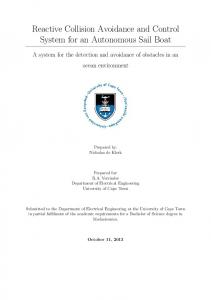
Figure 3D3D obstacles are are sorted in height bandsbands according to the 3Dtoshape Figure1.1. obstacles sorted in height according the of the robotof the robot. 3D shape
The has been been added added to to MRPT MRPT[3] [3]and andisis The implemented implemented code code has available under an open-source licence. Two demonstra‐ available under an open-source licence. Two tion videos of our approach, with the code, canthe be demonstration videos of ourtogether approach, together with found here: http://mapir.isa.uma.es/mjaimez code, can be found here: http://mapir.isa.uma.es/mjaimez 2.2.Related Related work work The navigation was was probably probably The first first example example of of reactive reactive navigation given [4]. From From then then on, on,reactive reactive given by by the the tortoises tortoises of of Walter Walter [4]. navigation and some some authors authors like like navigation has has been been well well studied, studied, and Brooks lowest hierarchical hierarchicallayer layer Brooks [5] [5] have have defined defined it it as as the the lowest of first successful successful methods, methods, of aa robotic robotic motion motion control. control. The The first such VO [8], [8], enabled enabled robots robots toto such as as VFF VFF [6], [6], VFH VFH [7] [7] and and VO advance toward a given target while avoiding the obstacles advance toward a given target while avoiding the encountered along the path, but they ignored both robot obstacles encountered along the path, but they the ignored shape kinematic Afterwards, reactive both and the its robot shape constraints. and its kinematic constraints. algorithms overcome these simplifications, Afterwards, started reactive to algorithms started to overcome these solving the navigation in a velocity space where simplifications, solvingproblem the navigation problem in a kinematic and dynamic constraints be easily consid‐ velocity space where kinematic and can dynamic constraints ered (typically, speed and acceleration limits). Within this can be easily considered (typically, speed and acceleration category, Simmons proposed to compute the optimal limits). Within this [9] category, Simmons [9] proposed to motion in amotion curvature-velocity where computecommand the optimal command in aspace curvaturetranslational rotational velocities are represented velocity spaceand where translational and rotational velocities independently. In a similar way, the “Dynamic Window Approach” (DWA) [10], which was arguably the most successful strategy of this kind, minimizes an energy function to obtain the best motion command regarding the reachable obstacles and velocities within a short time interval. DWA is still in use today thanks to its implemen‐ tation as a local planner in the popular Robot Operative System (ROS) “navigation” stack. These two approaches [9, 10] impose the feasible trajectory to be composed of circular arcs, so non-holonomic restrictions are also regarded, although, on the other hand, both the robot and the obstacles are still supposed to be circular. This circular shape assumption is also made in the extension of the Velocity Obstacle method [11].
Later improved solutions incorporated the robot shape into the reactive navigator. Minguez and Montano [12] defined the Ego-Kinematic Transformation (EKT): a mathematical procedure to transform the 3D configuration space into a new 2D space which implicitly contains the robot shape and its non-holonomic constraints. In this reduced space, the robot is a free-flying point and any holonomic obstacle avoidance method can be used to compute the solution. However, this approach still has a shortcoming: only circular paths are considered. This methodology was extended by Blanco et al. [2] with the generalization of path models through a novel approach called “Parameterized Trajectory Generator” (PTG). With this tool, several customized path models can be used in the reactive navigator and, at each iteration, the best one is selected according to some specific criteria, such as the collision-free distance for the selected movement, the minimum distance from the path to the target, etc. It must be noted that the robot becoming a free-flying point in this space comes at the cost of having a different set of obstacles in the trans‐ formed space, even for real stationary obstacles. However, as will be seen experimentally, this obstacle transformation can be made extremely efficient by means of precomputed look-up tables. In this context, reactive navigators were effective enough, but they still had to assume that the world was 2D. None‐ theless, the improvement and availability of 3D range sensor during the last few years have made it possible to realistically tackle the problem of navigating in 3D envi‐ ronments. Most of the new approaches are based on processing 3D point clouds and use the resulting informa‐ tion to execute a 2D navigator. For example, the solution proposed by Surmann et al. [13] consists in scanning the environment with a tilting laser and extracting some semantic information (planes) which is projected onto the floor plane and utilized by a 2D navigator. Holz et al. [14] also use a tilting laser to generate 3D point clouds, which are processed to obtain the “2D Obstacle Map” and “2D structure Map”. The former contains the minimum dis‐ tance in each scan direction (i.e., closest obstacles) and is exploited by the reactive navigator, while the 2D Structure Map contains the maximum distance in each scan direction (i.e., furthest obstacles) which is likely to correspond to the environmental bounds and is used for robot localization. In contrast, Marder-Eppstein et al. [15] proposed to store the 3D information in a voxel grid: a 3D occupancy grid whose cells are marked as occupied, free or unknown. The robot navigation is controlled by two modules: the “global planner” and the “local planner”. The “global planner” creates a high-level plan for the robot to reach the goal location and the “local planner” is a reactive navigator based on the aforementioned DWA [10]. No information is given about how the 3D voxel grid is interpreted by the 2D reactive navigator. Finally, the work recently proposed by Gonzalez-Jimenez et al. [16] addresses the problem of adding the 3D information provided by an RGB-D camera to a reactive navigator which was designed to work with
radial laser scanners. To this end, they propose to adapt the Kinect depth image into a virtual 2D scan which, in turn, encapsulates the 3D world information. From a different point of view, 3D navigation is also studied for legged robots and humanoids [17, 18, 19]. In these cases, point clouds are always analysed to extract semantic information, which is more convenient for the gait of this type of robot. In general, a 3D representation of the world has proved to be advantageous in many other aspects of the robot navigation, e.g., in localization [20]. 3. Reactive navigation based on PTGs For the sake of completeness, this section summarizes the PTG-based reactive navigator upon which our proposal for dealing with a 3D world is built. More details can be found in [2]. The PTG-based reactive navigator is based on a mathematical transformation that reduces the dimension‐ ality of the Configuration Space (C-Space) [21] from 3D ( x, y, ϕ ) to 2D, incorporating in the transformation the geometrical and kinematical constraints of the robot. The robot thus becomes a free-flying point over this 2D mani‐ fold embedded in C-Space, and the collision avoidance problem is easier and faster to solve. This dimensional reduction is accomplished by restricting the robot motion to one of a set of parametric path models which are compliant with the robot kinematics (e.g., circular paths, as shown in Figure 2). The set of all possible robot poses according to any path model constitutes a 2D manifold (“sampling surface”) embedded in the general C-Space (3D). The basic idea behind PTG-based navigation is to map those manifolds by means of 2D “Trajectory Parameter Spaces”, or TP-Spaces. The mathematical transformation between the TP-Space and the C-Space is formulated by a “Parameterized Trajectory Generator” or PTG, a smooth mapping of TP-Space points into C-Space poses according to a certain path model. TP-Spaces are expressed in polar coordinates, where the angle α corresponds to an individ‐ ual path from the family and the radius d indicates the normalized distance travelled along that path (Figure 2). The region of interest in a TP-Space is the circle of unit radius, that is, the sub-space A × D ⊂ ℝ2, where A = { α | α ∈ − π, π } and D = { d | d ∈ 0, 1 }. Therefore, kinematically compliant paths become straight lines in TPSpace and the robot motion can be guided with simple holonomic methods like VFF [6] or ND [22], disregarding the robot shape and non-holonomic constraints. Since several path models are included in the reactive system, several TP-Spaces are built. The mathematical transformation between the C-Space and the TP-Spaces is done by the inverse PTG function, defined as: -1
2
1
PTG : Sampling surface Ì R ´ S ® A ´ D Ì R
{( x , y ) ,f} ® (a , d )
2
(1)
Mariano Jaimez, Jose-Luis Blanco and Javier Gonzalez-Jimenez: Efficient Reactive Navigation with Exact Collision Determination for 3D Robot Shapes
3
Figure 2.Mathematical transformations from the Workspace (2D) to the C-Space (3D) and then to the TP-Space (2D). Individual Figure 2. Mathematical transformations from the Workspace (2D) to the C-Space (3D) and then to the TP-Space (2D). Individual trajectories (αa and αb) form trajectories a and αand b) form curves in C-Spacereferenced and are segments a particular referenced angle in the TP-Space. curves in the(α C-Space are segments forthe a particular angle in thefor TP-Space.
over this 2D manifold embedded in C-Space, and the Equation (1) transforms both obstacle points and the target collision avoidance problem is easier and faster to solve. from the C-Space to the corresponding TP-Space, using This dimensional reduction is accomplished by restricting path models such as those shown in Figure 3. In the the robot motion to one of a set of parametric path models resulting TP-Spaces, the robot becomes a free-flying point which compliant the robot kinematics (e.g., becauseare its shape and itswith kinematic constraints are embed‐ circular paths, as shown in Figure 2). The set of all possible ded into the mathematical transformation and, therefore, robot poses according any model constitutes a 2D any holonomic methodtocan bepath applied to get the best path manifold (“sampling surface”) embedded in the general Ci i αb in the i-th TP-Space. All the αb are subsequently evalu‐ Space (3D). The basic idea behind PTG-based navigation is ated and compared following some heuristic criteria which to map those manifolds by means of 2D “Trajectory take into account the collision-free distance for the selected Parameter Spaces”, or TP-Spaces. The mathematical movement, the minimum distance from the path to the transformation between the TP-Space and the C-Space is target, whether the robot will be heading to the target or formulated by a “Parameterized Trajectory Generator” or not, etc. The result of this process will be the most suitable PTG, a smooth mapping of TP-Space points into C-Space movement αb given the obstacles, the target and the path poses according to a certain path model. TP-Spaces are models being used. Finally, the speed commands associat‐ expressed in polar coordinates, where the angle ed with α are calculated and sent to the robot. This correspondsb to an individual path from the family and the sequence is repeated at a given frequency, typically higher radius indicates the normalized distance travelled along than 20 Hz, such that the robot can move smoothly. In that path (Figure 2). The region of interest in a TP-Space is summary, the PTG-based reactive navigator has two inputs the circle of unit radius, that is, the sub-space ⊂ , – the target relative pose and sensor data – and generates where | ∈ , and | ∈ 0,1 . one output: the velocity command for the robot. The Therefore, kinematicallycompliant paths become straight sequence of steps to compute the velocity commands is as lines in TP-Space and the robot motion can be guided with follows: simple holonomic methods like VFF [6] or ND [22], 1. For each path corresponding PTG, disregarding the model, robot using shapeits and non-holonomic transform the obstacles and the target to the associated constraints. SinceTP-Space. several path models are included in the reactive system, TP-Spaces built. The mathematical 2. For several each path model, are apply a holonomic reactive i transformation between the C-Space and the TP-Spaces is method to get the best path αb in the TP-Space. done by the inverse PTG function, defined as: 3. Select1 the best path αb among the candidates αbi 2 1 2 PTG : Sampling surface S A D obtained from the different TP-Spaces. (1) x , y , , d 4. Compute the linear and angular velocities and send Equation both unit. obstacle points and the target them(1) to transforms the robot motor from the C-Space to the corresponding TP-Space, using path models such as navigation those shown 4. PTG-based reactive in ain 3DFigure world 3. In the resulting TP-Spaces, the robot becomes a free-flying point The main limitation of a 2D navigator, such as the one because its shape and its kinematic constraints are described above or any of those reviewed in Section 2, is that both the robot and the world are assumed to be 2D, that is, the robot section is considered to be constant and the detected obstacles are projected onto the floor plane, 4
Int J Adv Robot Syst, 2015, 12:63 | doi: 10.5772/60563
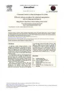
embedded into the mathematical transformation and, even if they are provided as 3D data by sensors like RGBtherefore, any holonomic method can be applied to get the D cameras or lidars. This happens to be a valid simplifica‐ in the i-th TP-Space. All the are best path tion under the assumption that the robot has roughly the subsequently evaluated and compared following some same horizontal profile all the way from bottom to top. heuristic criteria takerobots into account collision-free However, many which wheeled have athe non-constant distance for the selected movement, the minimum distance section (please visit ROS – robots to find many examples from the path to the target, whether the robot will like PR2, Gostai Jazz, Amigo, etc.), in which case the 2Dbe heading to the target or not, etc. The result of this process solution is suboptimal for two reasons: it takes the biggest given the obstacles, will be of the most suitable movement section the robot and also the closest obstacles regardless the target and the path models being used. Finally, of their height position in space. Figure 4 illustrates thisthe are calculated and speed commands with limitation with an associated obstacle configuration where a 2D sent to the robot. This sequence is repeated at a given reactive navigator would fail even though the robot has frequency, typically higher than Hz,ofsuch that the robot enough space to pass through. This20 kind situation is quite can move smoothly.In summary, the PTG-based reactive common in cluttered environments and demands the navigatorofhas – the (height) target relative pose and addition the two thirdinputs dimension to the reactive sensor data – and generates one output: the navigator in order to successfully cope with it. Forvelocity that commandwe formodel the robot. The sequence steps toacompute purpose, the robot geometryofthrough set of the velocity commands the is asrobot follows: prisms circumscribing volume, as shown in 1. For5. each path model,the using its corresponding Figure Besides defining 3D shape of the robot, itPTG, is obstacles and coordinates the target oftothethe also transform necessary tothe include the height obstacles or, more specifically, to sort them into height associated TP-Space. bands according to the height sections used to model the 2. For each path model, apply a holonomic reactive robot (Figure 1). Therefore, we decompose the 3D reactive in the TP-Space. method to get the best path navigator into N 2D navigators, N being the number of height sections Each 2D 3. Select the that bestmodel path the robot amonggeometry. the candidates navigator comprises andifferent individual robot section and the obtained from the TP-Spaces. obstacles in its corresponding height band. In order to 4. Compute thesolution linear and angular and the send obtain an overall for the robot,velocities we combine them to the robot motor unit. results for all the 2D navigators, as will be described later. At this point, it is necessary to give a brief explanation of 4. PTG-based reactive navigation in a 3D worldand what how obstacles are transformed into TP-Obstacles they represent (Figure 6). In the Workspace, obstacles are The main limitationtoofbea points. 2D navigator, such the one always considered Focusing on as a single described(orabove or and any given of those in Section 2, is obstacle point), its reviewed coordinates, the robot that both and we the can world are assumed be 2D, shape andthe its robot location, calculate all thetoposes robot section is considered to bebetween constantthe and (that x, y,is, ϕ ) the in the C-Space which imply a collision the detected are projected onto thefloor plane, robot and the obstacles obstacle. This set of poses forms a volume even C-Obstacle. if they Inare provided as to3D called addition, it is useful recalldata that inby C-Space every path model is a sampling surface. Thus, TPObstacles are obtained by transforming the 3D intersection between C-Obstacles and the sampling surface to the TPSpace.
this example example three different path models are considered, leading TP-Spaces. In bothTP-Spaces. the Workspace the the TP-Spaces the target Figure are considered,leading toInthree different TP-Spaces. In both themodels Workspace the to three different Figure 3. 3. In this three different path are and considered,leading to three different Inand both Workspace and the marked asin a green circle, while thefor obstacles are displayed in red.with The best for each TP-Space is shown with a blue arrow, and the best of all the three the obstacles areisdisplayed red. is The best path each TP-Space is shown a path TP-Spaces the target marked as a green circle, while the obstacles are displayed in red. The best path for each TP-Space is shown with a (PTG 3) is selected to provide the angular and linear robot velocities. cted to provide angular and linear bluethe arrow, and the bestrobot of allvelocities. the three (PTG 3) is selected to provide the angular and linear robot velocities.
Front view Top view pens to be a sensors like RGB-D cameras or lidars. This happens 2D approach to be a t the robot way fromvalid simplification under the assumption that the robot ots have ahas roughly the same horizontal profile all the way from to top. However, many wheeled robots have a ots to findbottom Conflicts Obstacles (tables) c.),in whichnon-constant section (please visit ROS – robots to find ons: it takesmany examples liked1PR2, Gostai Jazz, Amigo, etc.),in which the closestcase the 2D solution is suboptimal for two reasons: it takes 3D approach pace.Figurethe biggest section of the robot and also the closest anobstacle obstacles regardless of their height position in space.Figure would fail 4 illustrates this limitation with anobstacle ss through. configurationwhere a 2D reactive navigator dwould fail d 2 n cluttered the thirdeven though the robot has enough space dto pass through. n order toThis kind of situation is quite common in cluttered model theenvironments and demands the addition of the third cribing thedimension (height) to the reactive navigator in order to Figure4.4.Example Example of how theapproach 2D approach limits the navigator reactive Figure of how the 2D limits the reactive efining thesuccessfully cope with it.For that purpose, we model the navigator performance. performance nclude therobot geometrythrough a set of prisms circumscribing the 2 cifically, to ∈isℝnecessary Formally, letasσitshown be in a real in the Workspace, Atvolume, this point, toobstacle give brief explanation of robot Figure 5. aBesides defining the the height C-Obstacle(σ) its representation in C-Space and P a 3D point how obstacles are transformed into TP-Obstacles and what 3D shape of the robot, it is also necessary to include the erefore, we in C-Space. TP-Obstacles are defined they represent (Figure In the Workspace, obstacles areto coordinates of the 6). obstacles or, as: more specifically, to N 2Dheight always considered to be points. Focusing on a single them into height bands according to the height ctions thatsort obstacle (or point), and coordinates, the robot TP - Obstacle (s ) = the drobot P ) , Therefore, we (a ,given ) | (a , dits ) = PTG (1). used to model (Figure comprisessections (2) shape and its location, we can calculate all the poses 3D (sreactive navigator intobetween N 2D cles in itsdecompose C - Obstacle ) Çwhich Samplingimply surface , , "PinÎthe the C-Space a collision an overallnavigators, number height sections the robotNbeing and thethe obstacle. Thisof set of poses formsthat a r all the 2Dmodel the robot geometry. Each 2D navigator comprises α is Nevertheless, the closest obstacleitfor each path volume called only C-Obstacle. In addition, is useful to recall
where dm is the minimum distance of the pairs (α, d ) ∈ TPTop view Obstacles. Front view 2D approach
Obstacles (tables)
Conflicts
d1 3D approach
1
2
d1
d2 d2
Figure 4. Example of how the 2D approach limits the reactive navigator performance.
At this point, it is necessary to give a brief explanation of how obstacles are transformed into TP-Obstacles and what they represent (Figure 6). In the Workspace, obstacles are always considered to be points. Focusing on a single obstacle (or point), and given its coordinates, the robot Figure5.Example of 3D geometric ofrobot theGiraff robot shape and its location, we models can all the Figure 5. Example of 3D geometric models of thecalculate Giraff (right) and poses an relevant individual section and isthe obstacles in its that in C-Space every path a sampling surface. here robot as it marks themodel maximum distance the robot Rhodon (left) (right) and Rhodon , , in(left). the C-Space which imply a collision between Thus, TP-Obstacles obtained by transforming the 3D can travel along thatare path, always from origin, corresponding height band. In order tothe obtain anwithout overall the robot and the obstacle. This the setsame of poses a Returning to the 3D reactive navigator, processforms is intersection between C-Obstacles and the sampling collision. The set of we closest obstacles TP-Space issurface called solution for the robot, combine the in results for all the 2D volume called C-Obstacle. In addition, it is useful to recall followed N height of the in robot to obtain a a realsections obstacle the Workspace, Formally, let ∈for thebe to the TP-Space. α , its “TP-NavLimit”. If there is no obstacle navigators, as will be described later. along the path that in C-Space every path model each is a indicating sampling the surface. TP-Space with N sets of TP-NavLimits, TP-NavLimit is set to 1 (the maximum distance C‐Obstacle in the representation in C-Space and Pthea 3D 3D Thus,its TP-Obstacles byheight transforming maximum distance thatare the obtained robot at that section can normalized TP-Space), that is: point in C-Space. areHence, defined as: travel alongTP-Obstacles a given pathC-Obstacles model. thethe most restrictive intersection between and sampling surface α TP-NavLimits are used to build the TP-Space for each to the TP-Space. TP - NavLimit ( a ) = min {1, dm } (3)
{
-1
}
TP Obstacle( ) , d | , d PTG (Figure 7), that is:
1
P,
Mariano Jaimez, Jose-Luis Blanco and Javier Gonzalez-Jimenez: P C Obstacle (Collision ) Sampling surface Efficient Reactive Navigation with Exact Determination for 3D Robot Shapes
}
(2) 5
Nevertheless, only the closest obstacle for each path is relevant here as it marks the maximum distance the robot
F C S
W N re N in tr m n m
( )
{
( )}
TP - NavLimit a = min TP - NavLimit n a n
(4)
where n = 1, 2 … N are the height sections of the robot.
Figure6.A set of obstacles in the Workspace is transformed to the
eGiraff robot
raff robot
Workspace, orkspace, and P a 3D
P a 3D
P,
(2)
(2)
ach path is nce the robot path is gin, without the robot ace is called , without he path , its is called tance in the
path , its ce in the
s
(3)
,
ection can he most (4) TP-Space
robot.
(4)
bot.
6
Before applying the PTG transformations, a module called “Short-Term Memory” (STM) stores the position of close obstacles that might eventually become unseen by the robot sensors if they enter into their blind zone. This is particu‐ larly relevant for RGB-D cameras which have a narrow FOV and cannot detect obstacles at short distances. The STM module is implemented by N local occupancy grids centred at the robot pose onto which the 3D points within each slice in height are projected. The appropriate grid and cell sizes depend on the sensors used, the accuracy of the localization estimate, how cluttered the environment is, etc. The outputs of the STM block are sets of “virtual obstacles” whose coordinates are generated from those of the occu‐ pancy grid cells. These virtual obstacles are merged with the real ones coming from sensors and passed to the TPObstacle builder. Detailed information about the occupan‐ cy grids, their working principle and how they are implemented can be found in [16]. All the obstacles, real and virtual, are converted into TPObstacles for a number of path models and also for each height level. This results in K×N sets of TP-Obstacles and, subsequently, in K×N sets of TP-NavLimits. Then, the N sets of TP-NavLimits corresponding to each path model are combined, as explained in Section 4, yielding K TP-Spaces representing the robot navigability for each path model. Concurrently, the relative target location is also trans‐ formed to these TP-Spaces, where any holonomic method can be run, for example VFF [6] or ND [22], to get the most suitable path αbi for each path model i . The best path
candidate αb among all is then the one that maximizes an
objective function that trades off several navigational criteria:
collision in the real world, hence over-constraining the robot motion.
∈TP(3)
me process is , ∈TPt to obtain a ndicating the process is t section can o, obtain a the most cating the he TP-Space
Figure 6. A set set of obstacles in the Workspace is transformed to the C-Space Figure6.A ofaccording obstacles the Workspace is to the C-Space and,to toinato path family, toTP-Space thetransformed associated TPand, according a path family, the associated C-Space and, according to a path family, to the associated TPSpace. Space. We thatcalculating calculatingthe theminimum minimum TPWewant wish to to remark remark that of of allall TPNavLimits is not equivalent to projecting the most restric‐ We wish to remark that calculating the minimum of all NavLimits is not equivalent to projecting the mostTPtive 3D obstacles ontoequivalent theonto floor. that thethat TP-NavLimit NavLimits is obstacles not to projecting the TPmost restrictive 3D theGiven floor. Given the ofNavLimit each individual robot section information about of obstacles each individual robot section contains restrictive 3D onto thecontains floor. Given that the TPhow far this part of the robot could travel in the 3D world information about how far this part of the robot could NavLimit of each individual robot section contains travel in the 3D world according some according toabout some path models, the minimum of the them information how far thistopart ofpath themodels, robot could minimum of them shows how the whole robot could shows how the whole robot could navigate in the same travel in the 3D world according to some path models, 3D the navigate in it same 3D world, since itrestrictions encompasses the world, since encompasses motion of every minimum ofthe them shows the how the whole robot could motion restrictions of restrictions every part correspond of it.Thus, all these of part of it.Thus, these to poses navigate in the all same 3D world, since it encompasses the restrictions correspond to poses of the robot that would the robot that would implyofcollisions the motion restrictions of actually every part it.Thus, with all these actually imply collisions with the environment, whereas environment, whereas the typical 2Dthe obstacle projection is restrictions poses of robotto that would the typicalcorrespond 2D obstacletoprojection is prone creating prone to creating motion constraints that do not correspond actually imply collisions the environment, whereas motion constraints that do with not correspond to any potential to any potential collisionprojection in the realisworld, hence overthe typical 2D obstacle prone to collision in the real world, hence over-constrainingcreating the constraining the robot motion. motion constraints that do not correspond to any potential robot motion.
typically laser scanners and RGB-D cameras. As previously mentioned, these 3D obstacle points are sorted according to the different height sections employed to model the robot volume.
( ) i
a b = arg max åwi fi a b a
(5)
with wi being weighting coefficients and f i factors which measure:
Figure Example of of combination of TP-NavLimits for a robot Figure7. 7.Example combination of TP-NavLimits for a with robottwo height sections. PTG1 is related to the first height (blue) section and PTG2 with two height sections. PTG1 is related to thesection first height to the second one (red). The resulting TP-NavLimits (black) are calculated (blue) and PTG2 to the second one (red). The resulting TPas the minimum of the TP-NavLimits associated with each individual PTG.
NavLimits (black) ofarecombination calculated asofthe minimum of for the aTPFigure 7.Example TP-NavLimits robot NavLimits associated with each individual PTG. with two height sections. PTG1 is related to the first height section 5. Theand 3D PTG2 reactive (blue) to navigation the second framework one (red). The resulting TP5. The 3D(black) reactiveare navigation NavLimits calculatedframework as the minimum of the TPIn this section we describe the overall operation of the NavLimits associated with each individual PTG. reactive navigator. consiststhe of overall a number of steps In this section we It describe operation of which the reactive navigator. It consists of a number of steps which are executed periodically at a given frequency (Figure 8). 5. The 3D reactive navigation framework are inputs executed periodically at a given frequency The to the reactive system are the obstacles(Figure and the 8).The inputs to the reactive system are the obstacles and relative location of describe the target. of sensors In this section we theDifferent overall kinds operation of the the relative location of the target. Different kinds of providing 3D obstacle points can benumber used simultaneously, reactive navigator. It consists of a of steps which sensors providing 3D obstacle points can be used are executed periodically at a given frequency (Figure simultaneously, laser and RGB-D Int J Adv Robot Syst, typically 2015, 12:63 | doi: scanners 10.5772/60563 8).The inputs to the reactive system are the obstacles cameras. As previously mentioned, these 3D obstacleand
the relative location of the target. Different kinds of sensors providing 3D obstacle points can be used simultaneously, typically laser scanners and RGB-D
• f 1 : The collision-free distance of each candidate (in TPSpace).
• f 2 : The angular distance in the TP-Space between the target and the candidate.
• f 3 : The minimum distance between the target and the path candidate.
• f 4 : How different the new (tentative) and the previous
speed commands would be (to soften the robot motion).
Finally, the linear and angular velocities are derived from αb and sent to the robot motion control unit.
All the obstacles, real and virtual, are converted into TPObstacles for a number of path models and also for each height level. This results in K×N sets of TP-Obstacles and, subsequently, in K×N sets of TP-NavLimits. Then, the N sets of TP-NavLimits corresponding to each path model are combined, as explained in Section 4, yielding K TPSpaces representing the robot navigability for each path
motion). Finally, the linear and angular velocities are derived from and sent to the robot motion control unit.
Giraff is a differential wheeled robot and has been equipped with a Hokuyo URG-04LX-UG01 laser and a PrimeSense Carmine 1.09 RGB-D camera, both facing forwards. Rhodon is a heavier differential wheeled robot equipped with two laser scanners (one Sick LMS200 and one Hokuyo UTM 30-LX, facing forwards and backwards respectively), and one Kinect camera placed at the top of the robot and tilted downward with an angle of 50 degrees. 3D points provided by all the range sensors are expressed with respect to the robot coordinate system and then merged before feeding the reactive navigator. In this preprocessing stage, the fused point cloud is down sampled, retaining only the most restrictive points at each height band. The frequency at which sensor data are read is adjustable; in our experiments it ranges from10 Hz for the Hokuyo URG-04LX-UG01 (its maximum)to 30 Hz for the remaining sensors.Due to the lack of 3D sensory information at their back (Rhodondoes contain a Hokuyo Figure 8. Scheme of the 3D reactive navigator with K different path models and N height sections but it is only used for localization), the Figure8.Scheme of the 3D reactive navigator with K different path modelsfacing and Nbackwards height sections. robotsare not allowed to move backwards during the experiments. 6. Experimental setup and implementation details 6.1 Configuration of the 3D reactive algorithm
6. Experimental setup and implementation details The 3D reactive navigator has been intensively tested for
months in several scenarios to demonstrate its proper
Giraff and mobile robots (Figure The functioning. 3D reactiveThe navigator hasRhodon been intensively tested for 5) have been chosen to conduct the experiments, as their months in several scenarios to demonstrate its proper heterogeneous profiles appropriate test the 3D functioning. The Giraff andare Rhodon mobileto robots (Figure reactive navigator’s performance. In particular, the Giraff 5) have been chosen to conduct the experiments, as their robot has been deployed and utilized for more than a year in several real apartments in Spain as part of the EU project GiraffPlus [23] using the proposed method to reactively navigate between nodes of a pre-established roadmap.
Giraff is a differential wheeled robot and has been equipped with a Hokuyo URG-04LX-UG01 laser and a PrimeSense Carmine 1.09 RGB-D camera, both facing forwards. Rhodon is a heavier differential wheeled robot equipped with two laser scanners (one Sick LMS200 and one Hokuyo UTM 30-LX, facing forwards and back‐ wards respectively), and one Kinect camera placed at the top of the robot and tilted downward with an angle of 50 degrees. 3D points provided by all the range sensors are expressed with respect to the robot coordinate system and then merged before feeding the reactive navigator. In this preprocessing stage, the fused point cloud is downsampled, retaining only the most restrictive points at each height band. The frequency at which sensor data are read is adjustable; in our experiments it ranges from 10 Hz for the Hokuyo URG-04LX-UG01 (its maximum) to 30 Hz for the remaining sensors. Due to the lack of 3D sensory information at their back (Rhodon does contain a Hokuyo facing backwards but it is only used for localization), the robots are not allowed to move back‐ wards during the experiments.
As a general is surrounde by the PTG adjusted tak with thefron those at the to increase navigation s dynamics an and conserva On the oth implemented account the permitted, th trapped whe impeded. In backward slo the reactive n a few secon collisions) a changes or th
heterogeneous profiles are appropriate to test the 3D reactive navigator’s performance. In particular, thetheGiraff First, we need to define the heightalgorithm sections that model 7. Experimen 6.1. Configuration of the 3D reactive robot has been deployed and utilized for more than a year robot geometry (Figure 5). In these experiments we have in several real in sections Spain as ofthe the EU A wide varie First, we the need to apartments define height thatpart model modelled Giraff robotthe with four consecutive prisms and first two sets robot geometry (Figure 5). In these experiments we have project GiraffPlus [23] (see using the 4 proposed method for Rhodon with five prisms Section for further details). modelled the Giraff robot withfourconsecutive prisms Second, path models and their characteristics have to be 3D navigato reactively navigating between nodes of a pre-established andRhodon with five prisms (see Section 4 for further specified; in our case three different path models are many roboti roadmap. details). Second, path9): models and their considered (Figure circular arcs,characteristics trajectories have with to be specified; in our case three different path models are asymptotical heading and trajectories with a minimal considered (Figure 9): circular arcs, trajectories with turning radius (see [2] for more details about their mathe‐ asymptotical heading and trajectories with a minimal matical definition). turning radius (see [2] for more details about their mathematical definition).
environment proposal,the specific and addressed w experiments, laser scanner of localizatio [24]. Those g environment registration o
7.1. Computa Figure9. Set of path models considered in the experiments by the
Figure 9. Set of path models considered in the experiments by the reactive reactive navigator. navigator
Furthermore, the the holonomic holonomic method Furthermore, method can can be be chosen chosenfrom from two options:VFF [6] or ND [12], and their two options: VFF [6] or ND [12], and their associated associated parameters can can be be customized customized too. too. We We opted opted forthe parameters for theND ND method because, in general, it outperforms method because, in general, it outperforms the the VFF. VFF. Finally, the reactive loop frequency is set to 20 Hz, which Finally, the reactive loop frequency is set to 20 Hz, which is fast enough to react to incoming sensor data without is fast enough to react to incoming sensor data without overloading the processor. overloading the processor. 6.2. Speed regulation and recovery behaviour
6.2 Speed regulation and recovery behaviour Linear and angular velocity commands sent to the robot
Linear and angular commands sent to path, the robot come from the PTG velocity associated with the selected but come themodulatedor PTG associated withwithout the selected path,the but they from can be rescaled violating
kinematic constraints of that path. Mariano Jaimez, Jose-Luis Blanco and Javier Gonzalez-Jimenez: Efficient Reactive Navigation with Exact Collision Determination for 3D Robot Shapes
In order to reactive navi complete ite Giraff robot 2.10GHz wit sections and iteration tak which impl milliseconds frequency. T other robotic which have t We can com navigator, i. model the ro milliseconds 7
they can be modulated or rescaled without violating the kinematic constraints of that path. As a general rule, the robot should move carefully when it is surrounded by obstacles, but this is not always granted by the PTGs. For this reason, the speed commands are adjusted taking into account the proximity of obstacles, with the frontal obstacles having a greater influence than those at the sides. This speed regulation, which allows us to increase the average robot speed while keeping the navigation safe, can be adjusted depending on the robot dynamics and the desired balance between robot agility and conservativeness. On the other hand, a basic recovery behaviour is imple‐ mented in case the robot gets stuck. Taking into account the fact that backward movements are not permitted, the reactive navigator assumes that the robot is trapped when both forward movements and rotations are impeded. In such situations, the robot starts to move backward slowly until it finds a feasible movement from the reactive navigator. If it is unable to find a way out after a few seconds, it stops (to avoid possible backward collisions) and keeps waiting until the environment changes or the user takes control of the situation. 7. Experiments A wide variety of experiments have been conducted. The first two sets are intended to study the performance of the 3D navigator under circumstances that are habitual in many robotic applications: navigation in an office-like environment and navigation at home. To validate our proposal, the other two sets of experiments include some specific and demanding situations that cannot be ad‐ dressed without 3D knowledge of the world. In all the experiments, localization relies on wheel odometry and laser scanners, which feed a particle filter implementation of localization based on a metric map of the environment [24]. Those geometric maps were previously built for each environment by means of a simple ICP-based incremental registration of laser scans.
8
the robot. In this case the reactive iteration takes 3.4 milliseconds, which implies that the 3D version is about 40% slower than the 2D for this particular configuration. The difference in time is not proportional to the number of height sections because, within one complete iteration of the 3D reactive approach, there are only a few steps that are executed for each height section of the robot model, as can be seen in Figure 8. 7.2 Navigating in an office-like environment The Giraff robot has navigated autonomously around our lab floor for more than a year, mainly in an area which includes a long corridor, our two-room lab and the two contiguous labs. This scenario presents a wide variety of static and dynamic obstacles that the robot has to detect and dodge (Figure 10). Apart from the geometric map for localization, the robot is provided with a topological map from which navigational targets are generated randomly. Table 1 shows the results of some of these navigational missions where navigational data were monitored to evaluate the reactive navigation performance. Overall, the robot has travelled 13.5 km with an average speed of 0.32 m/s and a top speed of 0.7 m/s. The incidents that took place during these sessions were classified into two categories. The first one, called “minor incidents”, refers to smooth contacts or grazes that the robot itself can manage and solve autonomously without human intervention. The second category comprises those cases where the robot gets stuck and cannot resolve the situation by itself, needing human intervention. Distance
Average
travelled
speed
(m)
(m/s)
5330
1771
1352
399
597
Minor
Human
incidents
intervention
0.332
0
0
0.295
0
0
184
0.308
1
0
564
179
0.317
0
0
7.1 Computational burden
1500
479
0.319
1
0
In order to check the computational resources that the reactive navigator demands, we have tested how long one complete iteration of the reactive module takes on the Giraff robot, whose processor is an Intel i3 – 2310M 2.10 GHz with 4.0 GB of RAM. Considering four height sections and three different path models, the reactive iteration takes 4.8 milliseconds on a single CPU core, which implies a computational load inferior to 100 milliseconds per second for the 20 Hz implemented frequency. This leaves more than 90% of the CPU to the other robotic modules (locali‐ zation, sensing, interface, etc.) which have to share the same computational resources.
1737
535
0.308
0
0
4749
1435
0.302
1
1
3974
1206
0.303
1
1
3764
1207
0.321
1
0
1614
537
0.333
2
0
5450
1811
0.332
4
0
4975
1587
0.319
5
1
1840
601
0.327
3
0
5228
1571
0.300
1
1
We can compare this runtime with that of the 2D reactive navigator, i.e., considering only one height section to model
11.854 h
20
4
Int J Adv Robot Syst, 2015, 12:63 | doi: 10.5772/60563
Duration (s)
Overall Results 13.5 km
0.316
Table 1. Results of the experiments in an office-like environment
The incidents recorded are explained according to their nature:
iguration. number of terationof steps that model, as
ound our rea which d the two variety of to detect c map for gical map ndomly. vigational itored to verall, the ed of 0.32 that took into two ”, refers to n manage ntion. The the robot by itself,
• Minor incidents are due to wheel slippage and the relatively Minor incidents are due slippage and the high response timetoof wheel the whole system. Wheel relatively high response time of the and whole slippage depends on the robot mechanics the system. surface slippage on the the robot mechanics itWheel is moving on, depends and causes to move inand an the surface way. it is moving on, and causes the checked robot to uncontrolled On the other hand, we have move an uncontrolled On the other hand, we that theinelapsed time fromway. the moment an obstacle is have checked thattime the the elapsed from the moment detected until the robottime starts to react to it is an obstacle is detected until the This timelatency the robot starts to slightly higher than 0.5 seconds. is the sum to it is ofslightly than 0.5 seconds. ofreact a number small higher response times, inertias, This and latency is the delays sum ofbetween a number of small communication modules of theresponse robotic times, inertias, and communication delays between architecture. modules of the robotic architecture. • Human intervention is mainly needed when the robot gets Human is mainlyneeded when the being robot stuckintervention due to unnoticed obstacles, most of them gets pieces stuck due to of unnoticed obstacles, small or part objects lying on themost floor.of them being small pieces or part of objectslying on the floor. Figure 10 gives an idea of how the robot has been wander‐ Figure 10 gives an idea of The howpoint the map robotshown has been ing during the experiments. was wandering experiments. The point shown built with during a laser the scanner and, hence, whitemap areas may was builtobstacles with a laser scannertoand, areas may contain invisible thehence, laser white scanner (tables, contain invisible to to thethelaser scanner (tables, chairs orobstacles other objects) but not RGB-D camera. This chairs or why otherinobjects) but notplot to the RGB-D camera. This explains the trajectory there are apparently free explains why the did trajectory plot there areapparentlyfree areas that thein robot not visit. areas that the robot did not visit.
Human ntervention
was lowered to 0.4 m/s in this case. The followed procedure is similar to that explained in the previous section: both metric and topological maps were built and provided to the robot which used them to navigate autonomously. Results are listed in Table 2. We can observe that the average speed has decreased, which is not only a consequence of the maximum speed reduction, but is also caused by the many situations in which the robot performs a pure rotation to turn round, contributing zero to the average velocity (see Figure 11 B). The incidents that took place during these tests are ex‐ plained following similar criteria to those mentioned in the analysis of the previous set of experiments: • Minor incidents are mainly due to the high response time of the robot working loop, which becomes more relevant when moving in tight spaces. • Only one human intervention was necessary because there were not many objects lying on the floor. Distance
Average
travelled
speed
(m)
(m/s)
3003
448
4331 3845
Duration
Minor
Human
incidents
intervention
0.149
2
0
644
0.149
2
0
571
0.149
1
1
4241
671
0.158
0
0
4263
654
0.153
1
0
4321
716
0.166
1
0
4384
731
0.167
3
0
3207
574
0.179
1
0
11
1
(s)
Overall Results
0
8.776 h
0
5.01 km
0.159
Table 2. Results of the experiments in a four-room flat
0
7.4 Navigation with an outstretched robotic arm
0 0 0 1 1 0 0 0 1 0 1
4
ronment.
g to their
Figure 10. A) Some of the robot navigating in an office-like Figure10.A) Somesnapshots snapshots of Giraff the Giraffrobot navigating in an environmentenvironment (first row) together withrow) a virtual representation robot office-like (first together with ofa the virtual and the obstacles detected by the sensors onboard (second row). B) The representation of the robot and the obstacles detected by the trajectory described by the robot during one of the missions. sensors onboard (second row). B) The trajectory described by the robot during one of the missions.
During this experiment, Rhodon is commanded to perform a task that would be unfeasible using a 2D navigator. This task consists in visiting different desks with a robotic arm in a stretched position, emulating the process of collecting and delivering objects autonomously, but omitting the manipulation phase as it is outside the scope of this work. This is an illustrative example of a robotic application that necessarily requires 3D knowledge of the environment and the robot. As PTG-based navigation does not support changeable robot shapes, the arm is maintained at the same position during the whole navigation so that the same five prisms model the robot shape properly throughout this test (if the arm moved, its corresponding height section could be modelled according to the range of motion of the manipulator). We specify a blind pixel region for Kinect and neglect all the points observed at that region of the
7.3 Navigating in a flat 7.3. Navigating in a flat As mentioned, the Giraff robot has been deployed for more than a year in several flats in Malaga (Spain) as part of the As mentioned, the Giraff robot has been deployed for objectives of the EU project GiraffPlus [23]. The flat selected more than a year in several flats in Malaga (Spain) as part for the experiments has four rooms and presents a narrow of the objectives of the EU project GiraffPlus [23]. The flat navigable space with a reduced margin for manoeuvre selected for the experiments has four rooms andpresents a (Figure 11). As a consequence, the Giraff maximum speed narrow navigable space with a reduced margin for manoeuvre (Figure 11). As a consequence, the Giraff Mariano Jaimez, Jose-Luis Blanco and Javier Gonzalez-Jimenez: maximum speed was lowered to 0.4 m/s in this Efficient case. The Reactive Navigation with Exact Collision Determination for 3D Robot Shapes followed procedure is similar to that explained in the
9
depth images since, given the camera pose on the robot (see Figure 5), the robotic arm is necessarily observed by the Kinect and would be considered an obstacle otherwise. Taking into account the weight (~ 50 kg) and height (1.8 m) of Rhodon, its maximum linear and angular speeds have been set to 0.4 m/s and 45 deg/s respectively. During the experiment, the robot has travelled 160 m around our lab visiting a total of seven different desks several times at random (Figure 12).
at different positions and giving it a target outside of the lab. Sometimes we put an additional piece of fabric crossing the contour so as to check that the robot realized it could not go across it. The maximum velocity was set to 0.3 m/s and the short-term memory (STM) was not used (please see the demonstration video at the link attached in the intro‐ ductory section).
maps were d them to le 2. decreased, mum speed ituationsin
Human intervention
0 0 1 0 0 0 0 0
1
urn round, gure 11 B). tests are ntioned in
h response omes more
ry because or.
manded to sing a 2D rent desks ulating the nomously, outside the mple of a knowledge PTG-based shapes, the 10 the whole the robot moved, its
Figure11. A) Some snapshots of the Giraff robot navigating in a
Figure 11. A) Some snapshots of the Giraff robot navigating in a flat (first flat (first row) together with a virtual representation of the robot Figure 12. A) Schematic map of the lab and the desks that Rhodon visited row) together with a virtual representation of the robot and the obstacles and the obstacles detected by the sensors onboard (second row). Figure12. A)theSchematic of the lab and the its desks that Rhodon during experiment. B)map Snapshots of Rhodon reaching destinations or detected by the sensors onboard (second row). B) The trajectory described B) the The trajectory described by theTherobot during of the round surrounded by obstacles (first row) together with a virtual by robot during one of the missions. geometric map one was built by visitedturning during the experiment. B) Snapshots of Rhodon reaching representation of the robot and the obstacles detected by the sensors missions. laser scans.The geometric map was built by laser scans. its destinations or row). turning round surrounded by obstacles (first onboard (second
according the range of motion the3Dmanipulator). We row) together with a virtual representation of the robot and the Aside fromtoaccomplishing its task,ofthe reactive naviga‐ specify a blind pixel region for Kinect and neglect all the We detected repeated this runsensors 20 timesonboard and the robot always passed obstacles by the (second row). tor has shown an improved behaviour with respect to the points observed at that region of the depth images since, through the silhouette if the blocking piece of fabric was 2D version since the robot was able, for example, to turn given the camera pose on the robot (see Figure 5), the not present and always stopped otherwise. Quite frequent‐ round when surrounded by chairs, tables or boxes while 7.5. Testing the reactive navigator’s limits robotic arm is necessarily observed by the Kinect and ly (about 50% of the times), however, the robot slightly the arm was moving above them. No incidents occurred would be considered an obstacle otherwise. Taking into touched the cloth as the field of view of the RGB-D camera during this test. In Figure 12 we can observe the final pose account the weight (~50 kg) and height (1.8 m) of Rhodon, is not wide enough to sense the whole clearance when the of the robot when it reached some of its destinations and its maximum linear and angular speeds have been set to robot gets close to the door (Figure 13). We also made some how the robotic arm lay above the corresponding desks. 0.4 m/s and 45deg/s respectively. During the experiment, trials activating the STM, but we found that using it had a the robot has travelled 160 maround our lab visiting a total counterproductive effect. As the localization module has a 7.5 Testing the reactive navigator’s limits of sevendifferent desks several timesat random (Figure precision of few centimetres, virtual obstacles are inserted 12). in the map carrying such positioning errors, which on A more extreme test to challenge the functioning of the 3D Aside from accomplishing task, the 3D reactive occasion prevents the robot from seeing the clearance or reactive navigator consisted ofitscommanding the robot to navigator has shown an improved behaviourwith cause undesired jittery behaviour in the reactive navigator. go through a contour which has the same profile respect as the to theitself. 2D version was forof example, to In this case, the errors in localization are higher than the robot For thissincethe purposerobot we cut outable, a piece fabric and turn roundwhen surrounded by chairs, tables or boxes spatial margins to pass through the clearance and, hence, placed it at the door frame (Figure 13). The experiment was while the arm was above No incidents the STM becomes useless. Nevertheless, the STM would be carried out placing themoving robot about 5 mthem. away from the door occurred during this test. In Figure 12 we can observe the final pose ofSyst, the2015, robot when reached some of its Int J Adv Robot 12:63 | doi: it10.5772/60563 destinations and how the robotic arm layabove the corresponding desks.
A rea go rob an wa do the cro it c 0.3 (pl the W thr no fre sli ca wh ma us mo ob err the rea
Figure12. A) Schematic map of the lab and the desks that Rhodon visited during the experiment. B) Snapshots of Rhodon reaching its destinations or turning round surrounded by obstacles (first row) together with a virtual representation of the robot and the obstacles detected by the sensors onboard (second row).
module has a precision of few centimetres, virtual obstacles are inserted in the map carrying such positioning errors, which on occasion prevent the robot from seeing the clearance or cause undesired jittery behaviourin the reactive navigator. In this case, the errors in localization
7.5. Testing the reactive navigator’s limits
Figure 13. Real images (up) (up) and representations of the robot, therobot, detected the mapand (down) how the robot goes the contour Figure13.Real images and representations of the theobstacles detectedand obstacles the showing map (down) showing howthrough the robot goes
through the contour.
a good solution as long as the robot pose was estimated arehigher than the spatial margins to pass through the more precisely. clearance and, hence, the STM becomes useless. Nevertheless, the STM would be a good solution as long as
8. Conclusions
We have presented a 3D reactive navigator that can be adapted to almost any robot moving on a flat surface. We achieve high levels of versatility and manoeuvrability, as only very weak assumptions have been made to formulate this 3D approach, namely: • The robot can be properly modelled in three dimensions as a set of prisms. • Measurements coming from different kinds of sensor can be directly merged and read by the reactive naviga‐ tor, provided they are expressed as 3D point sets. The robot is allowed to move according to several kine‐ matically compliant path models. Two robots with hetero‐ geneous height sections were chosen to test the reactive navigator in different environments. A fair amount of experiments were conducted and the results support its proper functioning, although it may be conditioned by some factors. First, the robot mechanics has been shown to play an important role and can spoil the reactive navigator performance if the robot is not able to reproduce the motion commands quickly and accurately enough. Second, the coverage of the surroundings by the robot sensorial system is also a key factor that clearly delimits the quality of the reactive navigator. The number, type and placement of sensors needed for the robot to comprehensively sample its surroundings are aspects that require a great deal of attention. In this respect, we believe that active perception could be an effective solution to improve obstacle detection without demanding many sensorial resources. Although it has not been contemplated here, active perception repre‐
sents a potential improvement and will be studied in future
the robot pose was estimated more precisely. works. 8. Conclusions
9. Acknowledgements
This work has been funded by the Spanish Government under project DPI1011-25483, the EU FP7 Programme under the GiraffPlus project, and the Spanish grant programmes JDC-MICINN 2011 and FPI-MICINN 2012. 10. References [1] Arkin R. (1999) Behavior-Based Robotics. Cam‐ bridge, USA: MIT Press. [2] Blanco JL, Gonzalez-Jimenez J, Fernandez-Madri‐ gal JA (2008) Extending obstacles avoidance methods through multiple parameter-space trans‐ formation. Autonomous Robots, vol. 24, no. 1, pp. 29-48. [3] Blanco JL. The Mobile Robot Programming Toolkit (MRPT) [Internet]. Available from: http:// www.mrpt.org, Accessed on 22 Dec 2014. [4] Walter WG (1953) The Living Brain. New York: Norton. [5] Brooks R (1986) A robust layered control system for a mobile robot. IEEE Journal of Robotics and Automation, vol. RA-2, pp. 14-23. [6] Borenstein J, Koren Y. (1989) Real-time obstacle avoidance for fast mobile robots. IEEE Transactions on Systems, Man and Cybernetics, vol. 19, no. 5, pp. 1179-1187. [7] Borenstein J, Koren Y (1991) The vector field histogram - fast obstacle avoidance for mobile
Mariano Jaimez, Jose-Luis Blanco and Javier Gonzalez-Jimenez: Efficient Reactive Navigation with Exact Collision Determination for 3D Robot Shapes
11
robots. IEEE Transactions on Robotics and Auto‐ mation, vol. 7, no. 3, pp. 278-288.
matics in Control, Automation and Robotics (ICINCO), Reykjavik, Iceland.
[8] Tychonievich L et al. (1989) A maneuvering-board approach to path planning with moving obstacles. Proceedings of the 11th International Joint Confer‐ ence on Artificial Intelligence, vol. 2, pp. 1017-1021.
[17] Morisset R et al. (2009) Leaving flatland: Toward real-time 3D navigation, Proceedings of the IEEE International Conference on Robotics and Automa‐ tion (ICRA), Kobe, Japan, pp. 12-17.
[9] Simmons R (1996) The curvature-velocity method for local obstacle avoidance. IEEE International Conference on Robotics and Automation, Minne‐ apolis, pp. 3375-3382.
[18] Nishiwaki K, Chestnutt J, KagamiS (2012) Autono‐ mous navigation of a humanoid robot over un‐ known rough terrain using a laser range sensor. The International Journal of Robotics Research, vol. 31, no. 11, pp. 1251-1262.
[10] Fox D, Burgard W, Thrun S (1997) The dynamic window approach to collision avoidance. IEEE Robotics and Automation Magazine, vol. 4, no. 1, pp. 23-33. [11] Fiorini P, Shiller Z (1998) Motion planning in dynamic environments using velocity obstacles. The International Journal of Robotics Research, vol. 17, no. 7,pp. 760-772. [12] Minguez J, Montano L (2006) Abstracting vehicle shape and kinematics constraints from obstacle avoidance methods. Autonomous Robots, vol. 20, no. 1, pp. 43-59. [13] Surmann H, Nuchter A, Hertzberg J (2003) An autonomous mobile robot with a 3D laser range finder for 3D exploration and digitalization of indoor environments. Robotics and Autonomous Systems, vol. 45. [14] Holz D, Lorken C,Surmann H (2008) Continuous 3D sensing for navigation and SLAM in cluttered and dynamic environments. Proceedings of the Interna‐ tional Conference on Information Fusion, Cologne, Germany. [15] Marder-Eppstein et al. (2010) The office marathon: Robust navigation in an indoor office environment. Proceedings of the IEEE International Conference on Robotics and Automation (ICRA). [16] Gonzalez-Jimenez J, Ruiz-Sarmiento JR, Galindo C (2013) Improving 2D Reactive Navigators with Kinect. In 10th International Conference on Infor‐
12
Int J Adv Robot Syst, 2015, 12:63 | doi: 10.5772/60563
[19] Gutmann JS, Fukuchi M, Fujita M (2008) 3D perception and environment map generation for humanoid robot navigation. The International Journal of Robotics Research, vol. 27, no. 10, pp. 1117-1134, 2008. [20] Kümmerle R et al. (2008) Monte Carlo localization in outdoor terrains using multilevel surface maps.Journal of Field Robotics, vol. 25, no. 6-7, pp. 346-359, 2008. [21] Lozano-Pérez T (1987) A simple motion-planning algorithm for general robot manipulators. IEEE Journal of Robotics and Automation, vol. 3, no. 3, pp. 224-238. [22] Minguez J, Montano L (2004) Nearness diagram (ND) navigation: Collision avoidance in trouble‐ some scenarios. IEEE Transactions on Robotics and Automation, vol. 24, no. 1, pp. 45-59. [23] Coradeschi S et al. (2013) Giraffplus: Combining social interaction and long term monitoring for promoting independent living. Proceedings of the 6th International Conference on Human System Interaction (HSI), pp. 578-585. [24] Blanco JL, Gonzalez-Jimenez J, Fernandez-Madri‐ gal JA (2010) Optimal filtering for non-parametric observation models: Applications to localization and SLAM. The International Journal of Robotics Research (IJRR), vol. 29, no. 14.