A practical method using spreadsheets is proposed for calculating the Hasofer-Lind second ... An advantage of the spreadsheet method is that partial derivatives.
Downloaded from ascelibrary.org by Indian Inst Of Science on 09/13/12. For personal use only. No other uses without permission. Copyright (c) 2012. American Society of Civil Engineers. All rights reserved.
EFFICIENT RELIABILITY EVALUATION USING SPREADSHEET By B. K. Low,t Member, ASCE, and Wilson H. Tang,2 Fellow, ASCE ABSTRACT: A practical method using spreadsheets is proposed for calculating the Hasofer-Lind second moment reliability index 13. Two example problems involving correlated normals and correlated nonnormals, respectively, are solved and compared with established mathematical approach. The proposed method is based on the perspective of an ellipsoid that is tangent to the failure surface in the original space of the random variables; concepts of transformed space or reduced variates are not required. Correlation is accounted for by setting up the quadratic form in the spreadsheet. Nonnormals are dealt with using established relationships between nonnormal distribution and its equivalent normal distribution. Iterative searching is performed automatically by invoking a spreadsheet's optimization tool. An advantage of the spreadsheet method is that partial derivatives are not part of the input; the method may therefore be especially attractive for cases with complicated or nonexplicit performance functions.
INTRODUCTION The second moment reliability index 13 as defined by Hasofer and Lind (1974) is generally considered to be a better approach in civil engineering design than the conventional factor of safety concept. The index reflects not only the effect of the mean values but also the covariances of the random variables influencing the design. The matrix formulation of the Hasofer-Lind index was given, for example, in Ditlevsen (1981), citing Veneziano (1974) I3HL =
min Y(x - m/C l(X - m)
(1)
xEF
where x is a vector representing the set of random variables; m = their mean values; C = covariance matrix; and F = failure region. A widely used procedure for computing the 13 index by (1) is to transform the failure surface into the space of reduced variates, whereby the shortest distance from the transformed failure surface to the origin of the reduced variates is the reliability index 13. The computation procedure is well explained in Ditlevsen (1981), Ang and Tang (1984), Madsen et al. (1986), Melchers (1987), Dai and Wang (1992), and Tichy (1993), among others. A more intuitive interpretation of 13 is possible by noting that (1) literally suggests that the Hasofer-Lind index can be calculated by minimizing the quadratic form (in this case an ellipsoid) subject to the constraint that the ellipsoid just touches the surface of the failure region F. The convenience and clarity of this perspective for the proposed spreadsheet method of calculating the reliability index are shown in this paper. Cases involving single performance function are considered here. The concept and procedure could be extended to systems with multiple performance functions.
ALTERNATIVE PERSPECTIVE OF HASOFER-LIND INDEX In the original space of the random variables, one can define a one-standard-deviation (1-0') dispersion ellipsoid by its canonical form if the variables are uncorrelated; each axis of the ellipsoid is parallel to a corresponding coordinate axis. When
there is correlation the dispersion ellipsoid is tilted. The equation of the tilted ellipsoid is given by the quadratic form in (1), namely (x - m/C-'(x - m)
(2)
This quadratic form is an ellipse for two-dimensional (2D) case and a hyperellipsoid for dimensions greater than three. Eq, (2) is plotted in Fig. 1 for a 2D case with mean values m, = m2 = 9, and standard deviations 0", = 3, and 0'2 = 2, for different values of correlation coefficient p. When x, and X2 are uncorrelated, (2) reduces to the familiar expression of an ellipse, the shape of which is labeled p = 0 in Fig. 1. When x, and X2 are correlated, the ellipse rotates and changes its aspect ratio. Despite the rotation, the dispersion of the 1-0' ellipse in the original X,-X2 reference frame is still defined by 0', and 0'2' The failure surface shown in Fig. 1 is a second degree polynomial, X2 = 25.5 - 1.4lx, + 0.039xi, and, for the case with correlation coefficient p = 0.7, a reliability index 13 equal to 2.18 is obtained using the spreadsheet method described in Low (1996), which will be explained and extended to correlated nonnormals in the next section. The 1-0' ellipse, the 130' ellipse, and the failure surface are plotted together in Fig,
18 16 14 12 X2
±
10
0.99
m2
8
0"2
6 4
'Sr. Lect., Civ. and Struct. Engrg., Nanyang Technol. Univ., Nanyang Ave., Singapore 639798. 2Prof. and Head, Civ. and Struct. Engrg., Hong Kong Univ. of Sci. and Technol., Hong Kong. Note. Associate Editor: Mahendra P. Singh. Discussion open until December 1, 1997. To extend the closing date one month, a written request must be filed with the ASCE Manager of Journals. The manuscript for this technical note was submitted for review and possible publication on June 10, 1995. This technical note is part of the Journal of Engineering Mechanics, Vol. 123, No.7, July, 1997. ©ASCE, ISSN 0733-9399/97/ 0007-0749-0752/$4.00 + $.50 per page. Technical Note No. 10929.
=1
2
~
0"1
m1
0
0
2
4
6
10
8
12
14
16
18
X1 FIG. 1. 1-0' Dispersion Ellipse Rotates as Correlation Coefficient p Changes JOURNAL OF ENGINEERING MECHANICS / JULY 1997/749
J. Eng. Mech. 1997.123:749-752.
Downloaded from ascelibrary.org by Indian Inst Of Science on 09/13/12. For personal use only. No other uses without permission. Copyright (c) 2012. American Society of Civil Engineers. All rights reserved.
18 ~ Jll§aO. ~
Unsafe region
16
Y Z M
14
28.857 46.479 1341.2
40 50 1000
5 2.5 200
Covariance Matrix 25 5
5 6.25 0
o
0 0 40000
12
X2
10
m2
8
6
gOO 1E·05
4 2
(
0 0
2
4
6
8
10
12
14
16
18
FIG. 3. mals
Solvet's default options used.
Spreadsheet Solution for Example 1, Correlated Nor-
X1
g(X)
FIG. 2. 1-0' Dispersion Ellipse and Critical Ellipse, for Correlation Coefficient p 0.7
=
)
= yz -
(4)
M
where Y = yield strength of steel; Z
= section
modulus; and
M = applied bending moment at the pertinent section. The
2. The equation for the ~-O' ellipse is (2), but with the right hand side (RHS) replaced by ~2, where ~ = 2.18 as calculated. In Fig. 2, the ellipse that is tangent to the failure surface is ~ times the size (in terms of axis ratio) of the 1-0' dispersion ellipse. This provides an intuitive meaning of the reliability index ~ in the original space of the random variables. The ellipsoid approach via spreadsheet is intuitively simple and transparent. In solving the constrained nonlinear optimization problem of (1) the user literally asks for the smallest ellipsoid that touches the failure surface; concepts of transformed space and reduced variates [often used in connection with (1)] are not necessary. There is a connection between the multivariate normal density function and the reliability index ~. In the 2D case the bivariate normal density function is (3)
where ~ is as defined in (1), without minimizing. Therefore, to minimize ~ (or ~2) is to maximize the value of the bivariate density function. The 1-0' dispersion ellipse and the ~-O' ellipse of Fig. 2 are contours of probability density function. To find the smallest ellipse (or hyperellipsoid, for multivariate case) that is tangent to the failure surface is then equivalent to finding the most probable failure point. This perspective is consistent with that of Shinozuka (1983) who stated that "the design point x* is the point of maximum likelihood if x is Gaussian, whether or not its components are uncorrelated." The proposed spreadsheet method is illustrated in the following two examples, for correlated normals, and correlated nonnormals, and compared with established mathematical procedures. Although Microsoft Excel (version 5 or 7) was used, it is likely that other spreadsheet softwares are (or will be) equally adequate for the tasks in hand.
EXAMPLE 1: CORRELATED NORMALS Ang and Tang [(1984), Example 6.9] analyzed the reliability of a steel beam section using an established mathematical approach. The performance function was
mean values and standard deviations of Y, Z, and M are known. Also, the variables Y and Z are assumed to be partially correlated, with correlation coefficient pyz = 004. In the proposed spreadsheet method, the mean values and the covariance matrix are tabulated as shown in the spreadsheet in Fig. 3. The diagonal terms of the covariance matrix are O'~, O'i, and O'~, respectively. The nonzero off-diagonal terms represent pyzO'yO'z. Subsequent steps are 1. Formulas are entered for the column vector [x-m] and the row vector [x_m]T, where x represents xvalues, and m represents mean values. The xvalues are set equal to the mean values initially. 2. The inverse of the covariance matrix is obtained using the spreadsheet's built-in MINVERSE function: a. Select any blank 3 X 3 cells; b. Type "=minverse(array)," where "array" is entered by selecting the 3 X 3 covariance matrix; and c. Press "Enter" while holding down "Ctrl" and "Shift." 3. Similarly, the spreadsheet's MMULT function is used to obtain the matrix product [C]-l[x-m], then [x_m]T
. [Cr 1[x-m].
4. The formulas of the reliability index, ~ = sqrt([x-m]T . [Cr 1[x-m]), and of the performance function, g(x) = (YZ - M), are entered based on xvalues. 5. Solver is invoked, to Minimize ~, By Changing xvalues, Subject To g(x) = o. The solution obtained by Excel's Solver in step 5 is as shown in Fig. 3. The ~ value of 2.863 is virtually identical to that (2.862) in Ang and Tang (1984). The spreadsheet approach is simpler and more intuitive because it does not involve eigenvalues and eigenvectors, orthogonal transformation matrix, reduced variates, or explicit partial derivatives.
EXAMPLE 2: CORRELATED LOGNORMALS AND TYPE I ASYMPTOTIC EXTREME A case involving correlated nonnormals was considered in Ang and Tang [(1984), Example 6.10]. The performance function is the same as (4), except that the variables Y and Z are lognormals, with correlation coefficient pyz equal to 0.4. The
750/ JOURNAL OF ENGINEERING MECHANICS / JULY 1997
J. Eng. Mech. 1997.123:749-752.
Downloaded from ascelibrary.org by Indian Inst Of Science on 09/13/12. For personal use only. No other uses without permission. Copyright (c) 2012. American Society of Civil Engineers. All rights reserved.
variable M is Type I extreme. The mean and standard deviations of Y, Z, and M are otherwise the same as those in Fig. 3. The spreadsheet solution for this case (Fig. 4) has the matrix setup of the quadratic form (as in Fig. 3) to account for correlation, and the calculations of the lognormal parameters A and , from the mean value and the coefficient of variation n [e.g. Ang and Tang (1975)] A
=In(mean) -
,= ~
0.5,2;
(Sa,b)
For any trial xvalue of a nonnormal variate, equivalent normal parameters (mN, UN) can be obtained using the established procedure of equating the cumulative probability and the probability density ordinate of the equivalent normal distribution with those of the corresponding nonnormal distribution at the particular xvalue of the random variable. For lognormals the following are obtained [e.g., Ang and Tang (1984)] m N = xvalue X (l-ln(xvalue)
+
UN = xvalue
A);
x,
(6a,b)
For variable M, the Type-I-extreme parameters are a and u, given by a
1T
= •y6(TM Ir = 0.006413;
= mM
u
0.5772 - --a
= 910
(7a,b)
in which the standard deviation of M«TM) is 200 and the mean of M(mM) is 1,000, as in Fig. 3. The mean (m N) and standard deviation (UN) for the equivalent normal distribution of M are obtained from the following equations [e.g., Ang and Tang (1984) Eqs. 6.2S and 6.26] m N = M* - (TN-l[F(M*)]' ,
(TN
= {-l[F(M*)]}
(8a,b)
f(M*)
where M* is in this case the value of M of a point on the failure surface g(Y, Z, M) = 0; ep-l[.] = inverse of the cumulative probability (CDF) of a standard normal distribution; F(M*) = original CDF evaluated at M*;