Efficient Rendering of Optical Effects within Water Using Graphics Hardware Kei Iwasaki †
Yoshinori Dobashi ††
Tomoyuki Nishita †
†
†† University of Tokyo Hokkaido University 7-3-1 Hongo, Bunkyo, Kita 13, Nishi 8, Kita, Tokyo, 113-0033, Japan Sapporo, 060-8628, Japan {kei-i, nis}@is.s.u-tokyo.ac.jp
[email protected]
Abstract The display of realistic natural scenes is one of the most important research areas in computer graphics. The rendering of water is one of the essential components. This paper proposes an efficient method for rendering images of scenes within water. For underwater scenery, the shafts of light and caustics are attractive and important elements. However, computing these effects is difficult and time-consuming since light refracts when passing through waves. To address the problem, our method makes use of graphics hardware to accelerate the computation. Our method displays the shafts of light by accumulating the intensities of streaks of light by using hardware color blending functions. The rendering of caustics is accelerated by making use of a Z-buffer and a stencil buffer. Moreover, by using a shadow mapping technique, our method can display shafts of light and caustics taking account of shadows due to objects. Keywords: Water, Shafts of Light, Caustics, Shadows, Graphics Hardware, Natural Phenomena
1 Introduction The creation of realistic images of natural scenes is one of the most important subjects in computer graphics. Accurate simulation of natural phenomena is required to generate realistic images. Of all natural phenomena, the realistic rendering of water, such as the sea and lakes, is one of the most essential components, so many techniques have been developed to represent water accurately. The generation of realistic images concerned with water can be categorized into two classes as follows: rendering water viewed from above the water surface and rendering underwater scenes. Many methods for rendering water viewed from above have been developed. On the other hand, there have been few works focusing on rendering underwater images. Underwater scenery can be very attractive, so several methods have been developed to create realistic underwater images.
There are several optical effects that are important in water, such as shafts of light, caustics, and shadows. Caustics are the light patterns that are formed on surfaces. Refracted light from waves in the water can converge and diverge, and this effect creates caustics and shafts of light due to the light that gets scattered from suspended particles. Scattering or absorption due to water molecules and suspended matter determine the color of the water. Shadows due to objects within water are necessary to increase realism. This paper proposes a new method for fast rendering of realistic images of scenes within water. Recently, highly efficient graphics hardware has become available and therefore several methods have been developed to generate realistic images of natural phenomena [1, 2, 6, 19]. Our method makes use of the advanced graphics hardware. Our method is based on Nishita’s method [11]. We have improved his method for use with graphics hardware. However, his method requires several minutes to create a single image. Therefore we have extended his method in order to accelerate the computation by using graphics hardware. Our method can display the shafts of light, caustics on objects, and shadows due to objects. The shafts of light are rendered by using hardware color blending functions. Caustics are calculated by making use of a stencil buffer. The shadow map technique is used to create the shadows of objects. In this paper, previous work is discussed in Section 2. In Section 3 we describe the method of modeling waves that we have adopted. In Section 4 we describe our rendering method for shafts of light using graphics hardware. Section 5 deals with caustics not only on planes but also on complex objects. In Section 6 we discusses the displaying of shadows using graphics hardware. Then examples and a conclusion are presented in Sections 7 and 8, respectively.
2 Previous Work The research on creating realistic images related to water can be categorized into two types. First, we shall review
the previous methods used for rendering water viewed from above. Then the methods for rendering underwater scenes are discussed. There are two main components to create realistic images of water. One is the modeling of waves. In 1986, Fournier and Reeves displayed coastal scenes [3] using Gerstner’s wave model [4]. Peachey [13] presented a new wave model that could simulate the behavior of approaching a sloping beach using a height field computed from Stokes’ wave model, with quadric surfaces to introduce asymmetry. In 1987, Ts’o and Barsky proposed a new method ”WaveTracing” and modeled waves using Beta-spline interpolation [21]. They also took wave refraction into consideration. Their wave model is based on Gerstner wave model. However, the oceanographic literature tends to downplay Gerstner waves as a realistic model of waves. Tessendorf proposed a statistical wave model which synthesizes sine and cosine waves [20]. The other component for rendering water images is the calculation of the water color. Kaneda et al. [8] proposed a method for rendering realistic water surfaces, taking into account the radiative transfer equation of light in water. Nishita et al. [10] obtained an analytical expression for calculating ocean color taking into account the single scattering of light. Premoze and Ashikhmin [14] recently presented a light transport approach. They simulated different ocean depths near islands and various types of ocean such as muddy ocean, deep coastal ocean, and tropical ocean. Concerning underwater images, methods for caustics, shafts of light, and the color of the water itself have been developed. Shinya et al. [17] proposed an algorithm for displaying caustics. They calculated the illumination distribution on surfaces in advance by using grid-pencil tracing. Watt [22] developed backward beam tracing. These methods use a kind of ray tracing algorithm, so it takes too much time to generate images. Stam proposed a method for generating caustics textures [18]. His method, however, cannot generate caustics on any object directly. Displaying shafts of light is one of the most important elements to simulate scattering of light. Therefore, many methods have been proposed. Regarding shafts of light in the atmosphere, Nishita et al. [9] proposed a shading model for scattering and absorption of light. Recently, Dobashi et al. presented a method for rendering shafts of light through gaps between clouds [1]. They also improved the method so that it can deal with not only parallel light sources but also point light sources [2]. As for shafts of light within water, Jensen et al. [7] displayed caustics and shafts of light using photon maps. In general, however, the method of photon maps takes too much time. In 1994, Nishita and Nakamae [11] presented a method for displaying caustics, shafts of light, and the color of the water using an accumulation buffer. They subdivided
the water surface into meshes and made illumination volumes. The illumination volume is calculated by sweeping refracted vectors at each lattice point of the mesh. Then they used the scan line algorithm for calculating the intensities of illumination volumes and stored them in the accumulation buffer. One of the advantages of this method is the ability to handle free-form surfaces, but it takes several minutes to create an image since the accumulation buffer used was not a graphics hardware buffer and the intensities of the illumination volumes at each scan plane have to be calculated. In recent years, with increasing the quality of graphics hardware, many researchers have proposed hardwareaccelerated methods. Stam proposed a method for rendering smoke in real time using 3D texture mapping [19]. Heidritch presented a shadow map method using the alpha test and projective texturing mapping technique [5]. We propose a fast method for rendering optical effects within water using advanced graphics hardware. In our method, we also use illumination volumes for displaying shafts of light. The illumination volume is divided into several volumes to be suitable for graphics hardware and the intensities of shafts of light can be calculated by using hardware color blending functions. Caustics are also rendered by making use of illumination volumes. We determine the intersection area between the illumination volume and objects by using a stencil buffer. Our method can handle shadows due to objects by the hardware-accelerated shadow map method.
3 Modeling of Waves Although the purpose of this paper is not the modeling of waves, we discuss the methods for the modeling of waves in this section. Modeling of waves is very important since shafts of light results from the convergence and divergence of refracted light at the water surface. Caustics patterns are also determined by the shape of waves. The wave model which we have adopted is a statistical wave model [20]. The statistical wave model represents the wave height as the decomposition of sine and cosine waves. The wave height h(x, t) at time t can be calculated by the following equation. X ˜h(k, t) exp(ik · x), h(x, t) = (1) k
where x is the horizontal position and k is the wave number vector. This equation can be calculated by Fast Fourier ˜ t) determine the Transforms. The Fourier amplitudes h(k, ˜ t) is based on Phillips spectrum, shape of the wave. h(k, which is calculated from the wind speed and direction. One of the advantages of this model is that wind-speed can be handled by users. Although this model cannot represent plunging waves because of the limitation of the height
field, the statistical wave model can generate various waves from calm waves on a sunny day to rough waves like the movie ”The Perfect Storm”.
4 Displaying Shafts of Light Calculating shafts of light within water, which arise from refracted light due to waves, is one of the optical effects within water. This is the phenomenon that refracted light gathers since waves on the water surface act like lenses. The incident light reaching the water surface consists of two components: direct sunlight and skylight. In our method, we take sunlight into account and regard skylight as an ambient light.
where T (θi , θt ) is Fresnel transmittance from an angle of θi to θt and δ(θi , θt ) is the function which has the value 1 when the direction of the refracted light is coincident with the direction of Pv Q, and is 0 when it is not. If the angle between the viewing ray and the normal of the water surface is greater than the critical angle, the incident light is the reflected light at a point on the water surface. We consider the light as an ambient light. Then we multiply the ambient light and the attenuation ratio due to water particles between P2 Pv and accumulate by integration of the scattered light between P2 Pv . The intensities of shafts of light are calculated by the integration term of Eq. (2). Let us denote the integration term as Ishaf t for simplicity. To calculate Ishaf t , we make use of the idea of illumination volumes [11].
4.1 Basic idea of intensity calculation
water surface
Here, we describe the method for calculating the intensity of light reaching the viewpoint. The scattering of light due to water particles has to be taken into consideration to display shafts of light. Our method is an improved version of Nishita’s method [11]. So, we explain this method briefly. Moreover, to simplify the explanation, we assume that there are no objects within the water in this section. Ii
θi
Ii P3
P2
Q θt
θi P1 θt
P z
L
φ
illumination volume
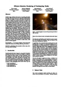
Figure 2. Illumination volume and subvolumes.
θ
y
sub-volume
l Pv viewpoint
Figure 1. Calculation of intensity reaching viewpoint. As shown in Fig. 1, when one’s viewpoint is located within the water, the intensity of light Iv (λ) coming from point Q on the water surface and reaching viewpoint Pv is calculated by the following equation. Z L Iv (λ)= IQ (λ)exp(−c(λ)L)+ IP (λ)exp(−c(λ)l)dl, (2) 0
where L is the distance between Pv Q, l is the distance between P Pv , c(λ) is the attenuation coefficient of light within water and IP represents intensity of light scattered at point P . If the angle between the viewing ray and the normal to the water surface is less than the critical angle, the intensity IQ is expressed by the following equation. IQ = T (θi , θt )(Isun (λ)δ(θi , θt ) + Isky (θi )),
(3)
As shown in Fig. 2, the water surface is subdivided into triangulated meshes. Then the refracted vector at each mesh point is calculated. The volume which is defined by sweeping the refracted vector at each point of the mesh is called the illumination volume (see Fig. 2). In the previous method [11], illumination volumes were sliced with each scan plane and the intersection area between an illumination volume and the scan plane was defined as the caustic triangle. The integration of scattered light equals to the sum of the intensities of caustic triangles which the viewing ray intersects. The second term of Eq. (2), Ishaf t , is approximated by the following equation. Z L X IP (λ)exp(−c(λ)l)dl = Ipi di exp(−c(λ)li ), (4) 0
i
where Ipi is the average intensity of the ith caustic triangle, di the intersected length of ith triangle and the viewing ray, li the distance between ith caustic triangle and the viewpoint. The scattered intensity IP (λ) at point P is calculated by the following equation. IP (λ) = (Ii T (θi , θt )Fp β(λ, φ)exp(−c(λ)ls ) + Ia )ρ, (5) where Ii is the intensity of incident light onto the water surface, T the transmittance at point P3 in Fig. 1, θi and θt are
the incident and transmitted angles, respectively. β(λ, φ) is the phase function, ρ the density, Ia the ambient light and Fp is the flux ratio between the intensity just beneath the water surface and at point on the caustic triangle since the energy of light in a caustic triangle is inversely proportional to its area. Nishita et al. calculate Ishaf t on a scan line basis. That is, Ishaf t was calculated by slicing the illumination volumes with each scan plane and summing the intensities of caustic triangles. A large number of illumination volumes are required to create realistic images. Therefore, their method is computationally very expensive. In the following subsections, our method to accelerate the computation of Ishaf t by using graphics hardware is described.
4.2 Proposed method for shafts of light The basic idea to render shafts of light is to display the shaded front faces of the illumination volume. The intensity of the illumination volume is calculated by integrating the scattered light along the intersection segment of the viewing ray with the illumination volume. However, the intersection test for each pixel requires a great deal of computational cost. So, as shown in Fig. 2, we subdivide each illumination volume into several volumes (we call these volumes sub-volumes). Since the intensity of sunlight, that is refracted at the water surface, is exponentially attenuated, the illumination volumes are subdivided so that the intensities of scattered light along the sub-volumes can be approximated linearly. This makes it possible to display the illumination volumes by using the Gouraud shading function. The sub-volume is further subdivided into three tetrahedra to integrate intensities of scattered light along the viewing ray within the sub-volume. We render the shafts of light by drawing these tetrahedra. We can reduce the computational time by the approximate calculation of the tetrahedron intensities as follows. As shown in Fig. 3, let us consider the sub-volume which consists of six points Pi (i = 1, ..., 6). Here we focus on the tetrahedron consisting of four points P1 , P2 , P3 and P4 . Geometrically, the tetrahedra projected onto the screen can be classified into two cases (see Figs. 4 and 5). Let P10 , P20 , P30 and P40 be the projected vertices of P1 , P2 , P3 and P4 , respectively. In case I the point P10 is inside the triangle 4P20 P30 P40 and in case II the point P10 is outside the triangle. In this section, we explain first the idea behind the proposed method for case I. Case II is described later. In the proposed method, shafts of light are rendered by displaying three triangles 4P10 P20 P30 , 4P10 P20 P40 and 4P10 P30 P40 and accumulating their intensities into the frame buffer. The intensities of pixels inside these triangles should be calculated by integrating the intensities of light scattered on the
P2 P2
P2
P3
P1
P3
P3
P1
P3 P5
P4 P5 P4
P6
P4 P4
P5
P6
Figure 3. Subdivide sub-volume into three tetrahedra.
intersection segments of the viewing ray with the tetrahedron. However, the intersection test for all pixels is very time consuming. Therefore we assume that the intensities of neighboring pixels are almost the same. This assumption is convincing if the illumination volume is sufficiently subdivided into small sub-volumes. Then, we calculate the intensities of four vertices, P10 , P20 , P30 and P40 only and the intensities of pixels inside the triangles are interpolated by using Gouraud shading function hardware. The intensities of these vertices are calculated as follows. In case I, the length of the intersection segment between the viewing ray and the tetrahedron is the longest when the viewing ray passes point P1 (see Fig. 4). We calculate IC which is the integrated of the scattered light arriving at the viewpoint for this longest case. On the other hand, since the intersection segment between the tetrahedron and the viewing rays for P20 , P30 and P40 is equal to 0, integration of the scattered light also gives 0. Therefore, we set the intensity of the vertex P10 to IC described before, and the intensities of the other vertices are set to 0. This method produces visually convincing results if the illumination volume is subdivided into small sub-volumes. In case II, as shown in Fig. 5, let point P70 be the intersection point between segments P10 P40 and P20 P30 . The length of the intersection segment is longest when the viewing ray passes point P70 . So, we calculate the integrated value IC along that segment. The intensity of point P70 is set to IC and the intensities of other vertices are set to 0. Then these four triangles 4P70 P10 P20 , 4P70 P10 P30 , 4P70 P20 P40 and 4P70 P30 P40 are displayed. In this way, we can reduce the computational time since our method does not require the intersection test between the viewing rays (or scan planes) and the illumination volumes used in the previous methods [11, 22]. Moreover, since our method renders shafts of light by displaying triangles, we can make use of graphics hardware to accelerate the computation. The outline of the process for rendering shafts of light is as follows.
P'2
1. Initialize the frame buffer. 2. Repeat the following process for each illumination volume.
P2
Pv P1
P'3
P3
P'1
Pb
(a) Subdivide the illumination volume into subvolumes. (b) Repeat the following process for each subvolume. i. Subdivide each sub-volume into three tetrahedra. ii. Project each tetrahedron onto the screen. iii. Classify the tetrahedron into two cases. iv. Calculate the intensities of the vertices of the triangles. v. Display the triangles and accumulate the intensities in the frame buffer. The classification of the tetrahedron is performed by investigating the geometric relation between the projected vertices of the tetrahedron. In the next section, we describe the calculation of IC . 4.2.1 Intensity calculation of tetrahedra of sub-volume The value of the integration, IC , described above is calculated as follows. First, we calculate the intersection points between the tetrahedron and the viewing ray passing through P10 (case I) or P70 (case II). There are two intersection points. Let these two intersection points be Pa and Pb , respectively. Let us denote the intensities at points Pa and Pb as Ia and Ib , respectively. In general, the length of the segment Pa Pb is very short, so we assume that the intensity in this segment Pa Pb varies linearly. Then, IC can be expressed by the following equation. IC =
Z
0
T
Ib − Ia Ia + Ib t + Ia dt = T, T 2
P4 P'4 (a)
(b)
Figure 4. Geometric relation of tetrahedron in case I.
4P1 P2 P3 (see Fig. 3) and Su is the corresponding area of the illumination volume at the water surface. Then intensity IPi at point Pi of the sub-volume is computed by the following equation. IPi (λ) = IPs i (λ)exp(−c(λ)li ),
(7)
where li is the distance between Pi and the viewpoint. The intensities of P4 , P5 and P6 can be calculated in the same way. 4.2.3 Intensity calculation in case I First, the two intersection points, Pa and Pb , between the viewing ray and the tetrahedron are calculated. In case I, Pa is equal to P1 . Pb is obtained by calculating the intersection of the ray with the triangle 4P2 P3 P4 (see Fig. 4). The intensity, Ia , of point Pa is given by Eq. (7). The intensity, Ib , of point Pb is calculated by interpolating the intensities of vertices P2 , P3 and P4 . The intensities of these vertices are also given by Eq. (7). 4.2.4 Intensity calculation in case II
(6)
where T is the distance between Pa Pb and t the distance between Pa and a point on the segment Pa Pb . Ia and Ib can be calculated by interpolating the intensities of the vertices of the sub-volume. We explain the calculation method for Ia and Ib in the following sections. First, we describe the calculation of the intensity at each sub-volume vertex. Then we present the calculation of the intensities Ia and Ib for case I and case II, respectively. 4.2.2 Intensity calculation of sub-volume Let’s consider a sub-volume shown in Fig. 3. First we calculate the scattered intensity IPs i at sub-volume vertex Pi (i = 1, ..., 3) by Eq. (5). The flux ratio in Eq. (5) is calculated by Fp = Su /Ss , where Ss is the area of triangle
In case II, the two intersection points, Pa and Pb , between the viewing ray and the tetrahedron are calculated as follows. Clearly, Pa is on segment P1 P4 and Pb on P2 P3 (see Fig. 5). Therefore, Pa is obtained by calculating the intersection point between the ray and the segment P1 P4 . Similarly, Pb is obtained by P2 P3 . Then, the intensity, Ia , of point Pa is obtained by interpolating the intensities of vertices P1 and P4 . The intensity, Ib , of point Pb is obtained from the intensities of vertices P2 and P3 .
5 Displaying Caustics 5.1 Intensity calculation for caustics To render caustics, we make use of illumination volumes again. Caustics patterns on objects are displayed by draw-
P'1 P2
5.2 Caustics on flat planes
Pb P3
P'2
P1
P'7
P'3
Pa
Pv
P4
1. Calculate the intersection points P1 , P2 and P3 between each illumination volume and the plane.
P'4
(a)
Let’s consider that the bottom of the water is flat as shown in Fig. 7. Caustics can be displayed by the following steps.
(b)
Figure 5. Geometric relation of tetrahedra in case II.
2. Calculate the intensity of each intersection triangle by Eq. (8). 3. Draw the intersection triangle 4P1 P2 P3 and accumulate its intensity into the frame buffer by using hardware color blending functions.
ing intersection triangles (caustic triangles) between illumination volumes and the objects. The intensity at each vertex of the caustic triangle, IPi , is calculated by the following equation. IPi = Ii T (θii , θti ) exp(−c(λ)(li + lv ))Fp Kobj cos γ, (8)
water surface
illumination volume bottom of water P2
where Ii is the intensity of the incident light, T (θii , θti ) is the transmittance at point Pis (see Fig. 6) on the water surface which corresponds to Pi , li is the distance between Pis and Pi (see Fig. 6), Fp is the flux ratio which can be calculated by the ratio of the area of the caustic triangle to the corresponding area of the water surface, Kobj is the reflectance of the object, γ is the angle between the object normal and the incident ray, and lv is the distance between Pi and the viewpoint. In the next section, we propose two methods for rendering caustics: caustics on planes and caustics on objects. Both methods can be accelerated by graphics hardware.
Ii θii Psi θti
water surface
li object normal object
Pi
γ lv
viewpoint
Figure 6. Intensity calculation of caustics on object.
P1 P3
Figure 7. Caustics on flat plane.
5.3 Caustics on objects The method for caustics on objects is not so easy as that for caustics on a plane. In this case, we have to investigate which illumination volume intersects the object. In the previous method [11], the caustic triangle between the illumination volume and the scan plane is calculated first. Then the calculation point on the object is checked to see whether the point is located within the caustic triangle or not. If the calculation point is within the triangle, the intensity of the calculation point is obtained by Eq. (8). To detect the points included in the caustic triangle, the depth of the triangle is compared with the depth of the objects. In the proposed method, the intersection test is accelerated by using the graphics hardware Z-buffer and stencil buffer. 5.3.1 Rendering caustics by using sub-volumes First, we make sub-volumes by slicing the illumination volumes with n scanplanes at a certain interval, ∆s. We call these scanplanes sample planes. That is, sample plane i (i = 1, ..., n) corresponds to scanline i∆s. Fig. 8(a) shows
sample plane i
stencil buffer
sub-voume object
stencil buffer sample plane i+1
scan plane
frame buffer (a) geometric relation between sub-volume and object
0 0 0 0 0 1 1 0 0 0 0 0 0
set to 1
object
(c) step 1
caustic triangle
object
(b) initial state
draw back faces further than object
scan plane
0 0 0 0 0 0 0 0 0 0 0 0 0
frame buffer
0 0 0 0 0 0 0 0 0 0 0 0 0
accumulate intensity if stencil value is 1
draw front face closer than object
reset to 0
object
scan plane
(d) step 2
Figure 8. Rendering caustics by using sub-volumes.
the geometric relation between the sub-volume and the object. To explain the proposed idea clearly, we show the rendering process on a scanplane (see Figs. 8(b), (c) and (d)). The drawing process of caustics is as follows. 1. Initialize the frame buffer and store the z values of objects in the Z-buffer (see Fig. 8(b)). 2. Draw the back faces of the sub-volume viewed from the viewpoint (see Fig. 8(c)). We do not draw the faces of the sub-volume in the frame buffer. We write 1 in the stencil buffer where the z values of the sub-volume are larger than the values of Z-buffer. In this step, we do not update the Z-buffer. 3. Draw the front faces of the sub-volume (see Fig. 8(d)). We accumulate the intensity in the frame buffer if the value of the stencil buffer equals 1 and the z values of the sub-volume are smaller than the values of the Z-buffer. In this step, we do not update the Z-buffer either. Step 3 of the above procedure is as follows. First, we calculate the intensities of the two caustic triangles which are the intersection areas between the illumination volume and sample planes i and i + 1 (see Fig. 8(a)). Next, we interpolate these two intensities by using the Gouraud shading
function which can be accelerated by graphics hardware. In this step, we reset the stencil buffer to 0 when we draw front faces in order to return the stencil buffer to the initial state. The above process creates an image of caustics on the objects. The value of each pixel represents the intensity of incident light on the objects. We call this image a caustic image. The final image is created by multiplying the pixel value by the surface reflectance and the cosine term (Kobj cos γ in Eq. (8)). To take into account this approximately, we calculate the refracted sunlight by assuming that the water surface is horizontal. The refracted sunlight is considered as a parallel light source. Then, an image of objects illuminated by this parallel source is created by using graphics hardware. The final image is obtained by multiplying this image and the caustic image. The multiplication of these images is done by using graphics hardware.
6 Shadows within Water In this section, we propose a method for rendering shadows due to objects within water. There are two types of shadows: shadows on the objects such as the ocean floor and shadows of shafts of light. In the proposed method, we display both of two types of shadows by the shadow map
method [15]. First, we assume that the water surface is flat. We calculate the refraction vector of sunlight. Secondly we generate a texture which is a depth image from the light’s point-ofview (i.e. a depth image viewed from the light source). The direction of the light is that of the refracted sunlight. Thirdly we render a scene from the eye’s point-of-view and store the depth values as a texture. Finally, we compare the values of the two textures and determine whether the corresponding pixel is shadowed or not. Applying the shadow map to displaying shafts of light and caustics can render shadows on objects and on shafts of light. The shadow map method can be accelerated by graphics hardware. However, the shadow map method has several disadvantages. The precision of the depth value stored in the shadow map is only 8-bit on a standard PC. It is not enough to render complex scenes. So we have adopted a 16-bit precision shadow map method by using a multidigit comparison [12]. Although this method works only on some graphics hardware, we are sure that this extension will in future be supported by much more graphics hardwares.
7 Examples Fig. 9 shows simple examples of a teapot within water. Figs. 9(a) and (b) show the teapot without and with shadows, respectively. Compared with Fig. 9(a), the shadows on the bottom of the water add reality in Fig. 9(b). Fig. 10 (see color plate) shows several examples of underwater optical effects. As shown in Fig. 10(a), shafts of light are obstructed by the teapot and shadows on the bottom of the water can be seen. Fig. 10(b) shows caustics on a submarine. This image indicates that our method can calculate caustics on objects with complex shapes. Figs. 10(c) and (d) are examples of a dolphin. Fig. 10(d) shows the dolphin viewed from the bottom of the water. Figs. 10(e) and (f) are stills from the animation of two dolphins. We created these images on a desktop PC (PentiumIII 1GHz) with Geforce2ULTRA. The image sizes of these figures are all the same, 640x480. The mesh size of the water surface is also all the same, 512x512. The number of illumination volumes is about 18,000. The number of subvolumes of one illumination volume is 20. The computational time for each figure is shown in Table 1. The computational time of Fig. 9(a) using software is 64 seconds. That is, the method using hardware is 22 times faster than the method using software. The motion of the dolphins in the animation is calculated by Free-Form Deformation [16]. These examples demonstrate that the proposed method can create realistic underwater images efficiently.
Table 1. Computation times Figure No. Time[sec](using hardware) Fig. 9(a) 2.92 Fig. 9(b) 4.07 Fig. 10(a) 4.45 Fig. 10(b) 5.81 Fig. 10(c) 4.34 Fig. 10(d) 4.55 Fig. 10(e) 5.10 Fig. 10(f) 5.37
8 Conclusion In this paper, we have proposed a method for rendering optical effects within water such as shafts of light, caustics on objects and shadows due to objects. The proposed method utilizes graphics hardware that has recently become highly efficient. We adopted OpenGL as a graphics library. The advantages of the proposed method are as follows. 1. Shafts of light are efficiently displayed by rendering illumination volumes which are subdivided into subvolumes. Sub-volumes are further divided into tetrahedra. Then, the shafts of light are displayed by drawing the visible triangles of the tetrahedra and accumulating their intensities. This process is accelerated by hardware color blending functions. 2. Our method can display caustics not only on flat planes but also on any object. To render caustics on objects, the intersection test between illumination volumes and the object is required. We detect the intersection regions by using a Z-buffer and a stencil buffer. 3. Shadows due to objects within water are also taken into consideration. There are two types of shadows: shadows on the objects and shadows due to shafts of light. We display both types of shadow by using the shadow map technique which can be accelerated by graphics hardware. In future work, we will improve the following subjects. First, we want to accelerate the proposed method in order to achieve real-time animations. Next, our shadowing method still has a room for improvement. Since we assume that the water surface is flat when calculating shadows, the boundaries of the shadows are sharp. Objects within water, however, are illuminated from various directions, so the boundaries of the shadows are not always sharp. Therefore we plan to render soft shadows.
(a) teapot without shadows
(b) teapot with shadows
Figure 9. Examples of a teapot within water.
References [1] Y. Dobashi, K. Kaneda, H. Yamashita, T. Okita, T. Nishita, ”A Simple, Efficient Method for Realistic Animation of Clouds,” Proc. SIGGRAPH2000, 2000, pp.19-28. [2] Y. Dobashi, T. Yamamoto, T. Nishita, ”Interactive Rendering Method for Displaying Shafts of Light,” Proc. Pacific Graphics2000, 2000, pp.31-37. [3] A. Fournier, W.T. Reeves, ”A Simple Model of Ocean Waves,” Proc. SIGGRAPH’86, 1986, pp.75-84. [4] F.J.v. Gerstner, ”Theorie der Wellen,” Ann. der Physik, 32, 1809, pp.412-440. [5] W. Heidrich, ”High-quality Shading and Lighting for Hardware-accelerated Rendering,” Ph. D. thesis, University of Erlangen, Computer Graphics Group. [6] W. Heidrich, H. P. Seidel, ”Realistic, Hardware-Accelerated Shading and Lighting,” Proc. SIGGRAPH’99, 1999, pp.171178. [7] H.W. Jensen, P.H. Christensen, ”Efficient Simulation of Light Transport in Scenes with Participating Media using Photon Maps,” Proc. SIGGRAPH’98, 1998, pp.311-320. [8] K. Kaneda, G. Yuan, Y. Tomoda, M. Baba, E. Nakamae, T. Nishita, ”Realistic Visual Simulation of Water Surfaces Taking into Account Radiative Transfer,” Proc. CAD/Graphics’91, 1991, pp.25-30. [9] T. Nishita, Y. Miyazaki, E. Nakamae, ”Shading Model for Atmospheric Scattering Considering Luminous Intensity Distribution of Light Sources,” Computer Graphics, Vol. 21, No. 4, 1987, pp.303-310. [10] T. Nishita, T. Shirai, K. Tadamura, E. Nakamae, ”Display of The Earth Taking into account Atmospheric Scattering,” Proc. SIGGRAPH’93, 1993, pp.175-182. [11] T. Nishita, E. Nakamae, ”Method of Displaying Optical Effects within Water using Accumulation-Buffer,” Proc. SIGGRAPH’94, 1994, pp.373-380.
[12] ”Shadow Mapping with Today’s OpenGL Hardware” GDC 2000, 2000, http://www.nvidia.com/developer.nsf/. [13] D. Peachey, ”Modeling Waves and Surf,” GRAPH’86, 1986, pp.65-74.
Proc. SIG-
[14] S. Premoze, M. Ashikhmin, ”Rendering Natural Waters,” Proc. Pacific Graphics’2000, 2000, pp.23-30. [15] M. Segal, C. Korobkin, R. Widenfelt, J. Foran, P. Haeberli, ”Fast Shadows and Lighting Effects Using Texture Mapping,” Computer Graphics, Vol. 26, No. 2, 1992, pp.249-252. [16] T.W. Sederberg, S.R. Parry, ”Free-Form Deformation of Solid Geometric Models,” Computer Graphics, Vol. 20, No. 4, 1986, pp.151-160. [17] M. Shinya, T. Saito, T. Takahashi, ”Rendering Techniques for Transparent Objects,” Proc. Graphics Interface’89, 1989, pp.173-181. [18] J. Stam, ”Random Caustics: Natural Textures and Wave Theory Revisited,” Technical Sketch SIGGRAPH’96, 1996, p.151. [19] J. Stam, ”Stable Fluids,” Proc. SIGGRAPH’99, 1999, pp. 121-128. [20] J. Tessendorf, ”Simulating Ocean Water,” SIGGRAPH’99 Course Note, Simulating Natural Phenomena, 1999, pp.1-18. [21] P.Y. Ts’o, B.A. Basky, ”Modeling and Rendering Waves: Wave-Tracing Using Beta-Splines and Reflective and Refractive Texture Mapping,” ACM Trans. on Graphics, 1987, pp.191-214. [22] M. Watt, ”Light-Water Interaction using Backward Beam Tracing,” Proc. SIGGRAPH’90, 1990, pp.377-385.
(a) teapot
(b) submarine
(c) dolphin(1)
(d) dolphin(2)
(e) two dolphins(1)
(f) two dolphins(2)
Figure 10. Examples of underwater scene.