flow graph (CFG) of basic blocks, which is derived with cur- rent methods ... this graph it is possible for paths to âcrossâ definitions; for ...... An API for runtime code.
Efficient, Sensitivity Resistant Binary Instrumentation Andrew R. Bernat and Kevin Roundy and Barton P. Miller Computer Sciences Department University of Wisconsin Madison, WI USA
{bernat,roundy,bart}@cs.wisc.edu
ABSTRACT
1.
Binary instrumentation allows users to inject new code into programs without requiring source code, symbols, or debugging information. Instrumenting a binary requires structural modifications such as moving code, adding new code, and overwriting existing code; these modifications may unintentionally change the program’s semantics. Binary instrumenters attempt to preserve the intended semantics of the program by further transforming the code to compensate for these structural modifications. Current instrumenters may fail to correctly preserve program semantics or impose significant unnecessary compensation cost because they lack a formal model of the impact of their structural modifications on program semantics. These weaknesses are particularly acute when instrumenting highly optimized or malicious code, making current instrumenters less useful as tools in the security or high-performance domains. We present a formal specification of how the structural modifications used by instrumentation affect a binary’s visible behavior, and have adapted the Dyninst binary instrumenter to use this specification, thereby guaranteeing correct instrumentation while greatly reducing compensation costs. When compared against the fastest widely used instrumenters our technique imposed 46% less overhead; furthermore, we can successfully instrument highly defensive binaries that are specifically looking for code patching and instrumentation.
Program instrumentation is a technique that injects new code into a program while attempting to preserve the visible behavior (that is, the output produced for a given input) of the original code. Instrumentation is a fundamental monitoring technology for areas such as cyberforensics [26], program auditing [27], precise behavior monitoring [18], attack detection [25], and performance analysis [23]. We address instrumentation of binaries, a program form that consists of only the code and data necessary to execute the program; binaries lack source code and often lack symbols and debugging information. In the commercial computing and security domains, the binary is frequently the only available form of a given program. Even in other domains, binary instrumentation may be necessary due to a lack of source code, binary-only vendor-provided libraries, or the need to instrument a program after it has been compiled and linked. Binaries are challenging to instrument, as they rarely contain sufficient space to insert instrumentation code directly. Instead, binary instrumenters must modify the structure of the binary to insert this new code. Current binary instrumenters have two significant weaknesses. First, they do not guarantee the instrumented binary will have the same visible behavior as the original [15]. Second, in their efforts to preserve this original visible behavior they may impose significant and unnecessary execution overhead by preserving aspects of the original binary’s behavior that do not impact its visible behavior. These two weaknesses have the same cause: the lack of a formal model of how the techniques they use to insert instrumentation impact the visible behavior of the original code. Instead, current binary instrumenters rely on ad-hoc approximations of this impact [2,3,14,17,20]. These weaknesses become particularly acute when instrumenting highly optimized code, hand-written assembly, or tamper resistant code. Highly optimized code or hand-written assembly may cause these approximations to improperly identify the impact of instrumentation, causing instrumenters to fail to preserve visible behavior. Tamper resistant code may attempt to purposefully subvert these approximations to ensure that instrumenting the tamper resistant binary will always affect its visible behavior. For example, we wrote a short program that determines the shape of its address space by identifying allocated memory pages; this program detects modification by widely used binary instrumenters. In this paper, we present a formal specification of how inserting instrumentation will affect the visible behavior of the instrumented binary. This specification allows instru-
Categories and Subject Descriptors D.2.5 [Software Engineering]: Testing and Debugging— Binary instrumentation
General Terms Experimentation, Languages, Performance
Keywords Binary instrumentation; Dynamic instrumentation; Binary rewriting; Static analysis; Binary slicing; Malware analysis
Permission to make digital or hard copies of all or part of this work for personal or classroom use is granted without fee provided that copies are not made or distributed for profit or commercial advantage and that copies bear this notice and the full citation on the first page. To copy otherwise, to republish, to post on servers or to redistribute to lists, requires prior specific permission and/or a fee. ISSTA ’11, July 17-21, 2011, Toronto, ON, Canada Copyright 2011 ACM 978-1-4503-0562-4/11/07 ...$10.00.
INTRODUCTION
menters to precisely determine which aspects of the original binary’s behavior they must preserve to ensure that its visible behavior is preserved. We formalize visible behavior as an approximation of denotational semantics that allows instrumentation to produce its own output. We describe a dataflow analysis that determines an overapproximation of the impact of instrumenting a binary on its visible behavior; this analysis can be used to replace the ad-hoc approximations used by current binary instrumenters. In our experiments, our approach imposed 46% lower overhead than widely used binary instrumenters and successfully instrumented highly defensive program binaries that attempt to detect any modifications of their code. Binaries rarely include sufficient space to insert instrumentation without moving original code. Instead, instrumenters create a copy of this code that is instrumented and execute the copied code instead of the original. This code is copied with a technique we call relocation that produces a new version that preserves the behavior of the original code but contains sufficient space to insert instrumentation. Relocating code alters the location of code within the binary and, as a side effect, alters the contents of registers and memory. These alterations may affect the behavior of instructions within the binary; we call such instructions sensitive. Examples of sensitive instructions include loads from modified memory (which may produce a different value) and branches that target the original location of moved code (which may incorrectly change control flow). We further subdivide sensitive instructions into two categories: externally sensitive instructions whose affected behavior will also cause the visible behavior of the binary to change, and internally sensitive instructions whose behavior will not. Whether an instruction is externally or internally sensitive cannot be derived from how the behavior of the instruction was affected by the code change; it also depends on how this behavior affects the surrounding code. For example, consider the effects of changing the location of a function that contains a call instruction. A call instruction saves the address of its successor; calls are sensitive to being moved because this address will change. Similarly, the return instructions in the callee are sensitive if they reference this address. If the only instructions that use the stored return address are these return instructions, then moving the call will not change the program’s control flow (and its visible behavior will not change). In this case, both the call and return instructions are internally sensitive. However, if this return address is used for another purpose (e.g., as output or as a pointer to data) then moving the call may affect visible behavior, rendering the call externally sensitive. Binary instrumenters strive to preserve the original visible behavior of the binary by identifying externally sensitive instructions during relocation and replacing them with sequences that compensate for any differences in visible behavior caused by these instructions. For example, an instrumenter may emulate a moved call instruction by first saving the original return address and then branching to the target of the call. This approach inposes overhead, which may become significant if the emulation sequence is frequently executed. For example, emulating all branches can impose almost 200% overhead [20], while doing so for all memory accesses as well can impose 2,915% overhead [6]. Therefore, the instrumenter should only add compensation code where necessary to preserve visible behavior from the effects of
externally sensitive instructions. In particular, overapproximating internally sensitive instructions as externally sensitive will impose unnecessary overhead, as these instructions do not change visible behavior. This work makes the following contributions: A model of instruction sensitivity: We describe a novel model of how relocation affects the behavior of instructions in the modified binary. Current relocation methods can be described as a combination of three basic operations: moving original code to new locations, adding new code to the moved code, and overwriting the original locations of moved code. We separate sensitive instructions into four classes based on the effects of these operations. Three of these categories represent instructions whose behavior is affected because their inputs are affected by modification: program counter (PC) sensitivity, code as data (CAD) sensitivity, and allocated vs. unallocated (AVU) sensitivity. The fourth category, control flow (CF) sensitivity, represents instructions whose control flow successors are moved. PC sensitive instructions access the program counter and thus will perceive a different value when they are moved. CAD sensitive instructions treat code as data, and thus will perceive different values if they access overwritten code. AVU sensitive instructions attempt to determine what memory is allocated by accessing unallocated memory and thus may be affected when new memory is allocated to hold moved and added code. CF sensitive instructions have had a control flow successor moved and thus may transfer control to an incorrect location. For each category of sensitivity we define how the inputs and outputs of the sensitive instruction are changed by modification. A formalization of compatible visible behavior: We define compatible visible behavior in terms of denotational semantic equivalence. Three characteristics of binary instrumentation render this frequently-undecidable problem tractable. First, since relocation only moves and adds but never deletes code there is a correspondence between each basic block in the original binary and a basic block in the instrumented binary. Second, we assume that executing added code will not change the behavior of the original code because executing instrumentation has no cumulative semantic effect on the surrounding code. Third, instrumentation does not purposefully alter the control flow of the original code, so the execution order of the instrumented binary will be equivalent to the original when the new locations of moved code are taken into account. We formalize these assumptions and define output flow compatibility, a stricter approximation of denotational semantic equivalence based on these characteristics. An analysis for identifying externally sensitive instructions: An externally sensitive instruction affects the behavior of the program in a way that causes the instrumented binary to fail output flow compatibility if the program is modified. We present an analysis that determines whether a sensitive instruction is internally or externally sensitive. We use symbolic evaluation [5] to determine how the sensitive instruction affects the output flow of the binary; if the output flow may change we conclude the instruction is externally sensitive. A framework for low-overhead compensation: Current instrumenters replace each instruction they believe to be externally sensitive with code that emulates its original behavior. This approach is straightforward but may miss
opportunities for greater efficiency. We describe an example group transformation that replaces a sequence of affected code as a single unit and results in a 23% decrease in overhead when instrumenting position-independent code (e.g., shared libraries). We have implemented the techniques described in this paper in the Dyninst binary analysis and instrumentation framework [3] and created a sensitivity-resistant prototype, which we call SR-Dyninst. Our instrumentation techniques will replace Dyninst’s instrumentation infrastructure in its next public release; in the meantime our source code is available upon request. This paper is organized as follows. We introduce our program representation and abstractions in Section 2. We present an overview of our instrumentation algorithm in Section 3, introduce our external sensitivity analysis in Section 4, and present our compensatory transformation algorithms in Section 5. We present performance results in Section 6, related work in Section 7, and conclude.
2.
NOTATION
We represent a binary program in terms of a process state, control flow graph (CFG), and data dependence graph (DDG). We use a conventional definition of a CFG as a collection of basic blocks connected by control flow edges. We extend the conventional definition of a process state to include input and output spaces; this extension allows us to represent an input operation as a read from an abstract input location and an output operation as a write to an abstract output location. Finally, the conventional definition of a DDG over binaries [10] may overapproximate data dependences between instructions that define multiple locations, as is common on real machines (Figure 1a). We provide more precise dependence information by splitting such instructions into sets of single-definition operations and using these operations as nodes in the DDG (Figure 1b). Process states (or simply states) are represented in terms of a set of abstract locations AbsLoc = Reg ∪Mem ∪In ∪Out. The registers Reg and memory Mem are defined conventionally; we assume the machine has a dedicated register pc that represents the program counter. For purposes of this work we refer to an IA-32 machine, though our approach is equally applicable to all architectures. We represent input and output with two sets of abstract locations In and Out. The set In = {in0 , . . . , inm } represents input to the program; we model each execution of an input operation (e.g., scanf) as an access of a unique input location. Output is similarly represented as the set Out = {out0 , . . . , outn }. A process state is a mapping from abstract locations to values; we use ⊥ to represent an unallocated abstract location. The input and output spaces of a program P are denoted In P ⊆ In and Out P ⊆ Out, respectively. We define the function Execute to relate program inputs and outputs as follows. Let the map x : In P → Values ⊥ represent an assignment of values to all locations in In P ; we refer to the set of all possible input assignments as Inputs P . Then the output produced by executing P on x is denoted by y = Execute(P, x) where the map y : Out P → Values ⊥ represents an assignment of values to all locations in Out P . We represent the control flow of a program with a control flow graph (CFG) of basic blocks, which is derived with current methods [8]. We denote the CFG of a program P as CF GP = (NP , EP ) where NP represents the set of blocks
Mem[sp]
r0
sp
Mem[sp]
i0: pop r0 sp
i0:r0
sp
i0:sp
i1:r1 r1
sp
i1:sp
sp
i1: pop r1 r1 i2: add r0, r1, r2
r0 sp
r2 i3: push r2 Mem[sp]
sp
sp
(a) Instruction nodes
i2:r2 r2
sp
i3: Mem[sp]
i3:sp
Mem[sp]
sp
(b) Operation nodes
Figure 1: Data dependency graphs. Figure (a) illustrates the problems of representing instructions as single nodes. In this graph it is possible for paths to “cross” definitions; for example, there is a path from the definition of r0 by i0 to the definition of the stack pointer sp by i3 , when in the actual program there is no such dependence. Our extended DDG, shown in (b), makes the intra-instruction data dependencies explicit and excludes erroneous paths. For clarity, we omit the condition register cc and the program counter pc.
and EP represents the set of edges. Executing a program traverses a path of nodes through the CFG; we denote this ExecPath(P, x) where x ∈ InputsP . We represent the data flow of a program with a data dependence graph (DDG). To provide more precise dependence information, we split instructions into a set of singledefinition operations. These operations form the nodes of our extended DDG. Formally, the DDG of a program P is a digraph DDG = (V, E). We use a virtual operation called initial to represent the initial assignment of abstract locations. A vertex in this graph is a pair of an instruction and an abstract location defined by that instruction, and the set of vertices is V = {(initial , a)|a ∈ AbsLoc} ∪ {(i, a)|i ∈ P ∧ a ∈ defs(i)}, where defs(i) represents the set of abstract locations defined by i. The set of edges E ⊆ V × V represents use-def chains between operations. We show an example of our extended DDG in Figure 1b. As with the CFG, we represent the DDG of a particular program P as DDG P .
3.
ALGORITHM OVERVIEW
This section presents our algorithm for sensitivity-resistant binary instrumentation that preserves the original visible behavior. To provide context, we compare our algorithm to a generic algorithm representative of existing binary instrumenters [2, 3, 17, 20]. These algorithms are compared and contrasted in Figure 2. Both our sensitivity-resistant algorithm and the generic algorithm are divided into three phases: preparation, code relocation, and program compensation. The preparation phase selects which code to relocate and allocates space for this code; this phase is the same in both algorithms. The code relocation phase copies the selected code, applies compensatory transformations to preserve its original behavior, and writes the transformed code into the program. The program compensation phase determines whether any non-selected instructions must also be transformed and applies appropriate transformations. Our work addresses two weaknesses in the generic algorithm. First, it may fail to correctly identify and transform externally sensitive instructions, thus failing to preserve the
Generic Instrumentation Algorithm Instrument(program, instCode, instPoint) // Preparation Phase codeToRelocate = SelectCode(program, instPoint) newAddr = AllocateSpace(codeToRelocate+instCode) // Code Relocation Phase relocCode = RelocateCode(codeToRelocate) program.Write(relocCode ∪ instCode, newAddr) // Program Compensation Phase transferCode = TransferToInstrumentation(instPoint)
Sensitivity Resistant Algorithm SR Instrument(program, instCode, instPoint) // Preparation Phase codeToRelocate = SelectCode(program, instPoint) newAddr = AllocateSpace(codeToRelocate+instCode) // Code Relocation Phase relocCode = SR RelocateCode(codeToRelocate) program.Write(relocCode ∪ instCode, newAddr) // Program Compensation Phase SR TransformExistingCode(program)
10: 11: 12: 13: 14: 15:
RelocateCode(codeToRelocate) foreach insn in codeToRelocate if IsPCorCFSensitive(insn) relocCode.insert(Emulate(insn)) else relocCode.insert(insn) return relocCode
SR RelocateCode(codeToRelocate) foreach insn in codeToRelocate if IsExternallySensitive(insn) relocCode.insert(SelectEfficientCompensation(insn)) else relocCode.insert(insn) return relocCode
16: 17: 18: 19:
TransferToInstrumentation(relocCode) foreach insn in codeToRelocate branch = GenerateBranch(insn.origAddr, insn.relocAddr) program.Write(insn.origAddr, branch)
SR TransformExistingCode(program) foreach insn in program if IsExternallySensitive(insn) program.Write(SelectEfficientCompensation(insn), insn.addr)
1: 2: 3: 4: 5: 6: 7: 8: 9:
Figure 2: A high-level overview of previous instrumentation techniques and our contributions. The left column presents a simplified view of the generic algorithm used by previous binary instrumenters. The right column presents our sensitivityresistant algorithm that maintains visible compatibility, with changes from the generic algorithm highlighted in bold.
original visible behavior. Second, it may apply compensation transformations to instructions that are not externally sensitive, thus incurring unnecessary runtime overhead. These weaknesses are due to the use of ad-hoc sensitivity identification techniques, and we address them by using analysis to identify which instructions are externally sensitive and transforming only these instructions.
Preparation phase. Instrumenting a sequence of code requires expanding the sequence to create sufficient space to insert instrumentation. Since this frequently can not be done in place, the code is instead relocated to newly allocated memory. We select which code will be relocated with a function SelectCode and allocate memory with a function AllocateSpace: SelectCode: This function identifies a region of code (e.g., a basic block or function) to be relocated. This region must cover at least the location being instrumented. Previous instrumenters have selected regions of varying sizes: a single instruction, basic block, group of basic blocks, or function. Our algorithm will successfully operate on any of these region sizes. AllocateSpace: This function allocates space to contain the combination of relocated code and instrumentation (e.g., by expanding the binary on disk or mapping additional memory at runtime). Previous instrumenters have assumed that allocating memory has no effect on the behavior of the program, which may not be the case if the program includes AVU-sensitive instructions. Our algorithm addresses this possibility by explicitly detecting AVU-sensitive instructions in its code relocation and program compensation phases.
Code Relocation Phase. This phase relocates the selected code to the memory allocated in the preparation phase, creating a sequence that should preserve the behavior of the original code. Previous instrumenters have done so with a function RelocateCode that identifies and compensates for PC- and CF-sensitive instructions, but that does not consider instructions to be CAD or AVU-sensitive. The assumption that instructions
are not CAD sensitive may be safe if the instrumenter ensures that original code is never modified [2, 17, 20]; however, assuming there are no AVU-sensitive instructions is not safe. Our analysis-driven algorithm instead uses a function SR_RelocateCode that uses analysis to identify all sensitive instructions, including CAD- and AVU-sensitive instructions. RelocateCode: This function examines each selected instruction (line 11), determines which instructions are PCand CF-sensitive (line 12), and replaces them with code that emulates their original behavior (line 13). All instructions that are not sensitive are copied without modification (line 14). This function produces a code sequence that will have the same behavior as the original when executed at the new address if all sensitive instructions were properly identified. RelocateCode also creates the appropriate space between relocated instructions to make room for instrumentation; this is not shown. For clarity, we describe this function in terms of a single pass; however, some instrumenters use a fix-point iteration to further optimize the relocated code. SR_RelocateCode: Our work improves RelocateCode by using analysis (represented by IsExternallySensitive, line 12) to identify externally sensitive instructions; this analysis is presented in Section 4. In addition, we attempt to select a more efficient compensation transformation than separately emulating each original instruction (represented by SelectEfficientCompensation, line 13); this function is presented in Section 5.
Program Compensation Phase. This phase attempts to preserve the original behavior of sensitive instructions that were not relocated, and has no effect if all code is relocated [2, 17, 20]. Previous patchbased instrumenters have used it to insert jumps to relocated code with a TransferToInstrumentation function [3,16]. This function does not consider the possibility of CAD- or AVUsensitive instructions in non-relocated code. We address this by instead using SR_TransformExistingCode, which uses our analysis to identify all externally sensitive instructions. TransferToInstrumentation: This function overwrites original code with branches to the corresponding locations
of relocated code (lines 18 and 19). This approach ensures that CF sensitive instructions do not affect the program’s behavior, but may cause incorrect program behavior if the program contains CAD sensitive instructions (as original code was overwritten). Any such CAD sensitive instructions are not handled. SR_TransformExistingCode: This function is similar in structure to SR_TransformRelocatedCode and shares many elements of its analysis. We examine each instruction (line 17) to identify the externally sensitive ones (line 18). We then apply an efficient compensatory transformation and write the transformed code to the program (line 19). For clarity, our description of this algorithm has assumed that the compensatory transformation does not increase the size of the code or affect the sensitivity of additional instructions. As these assumptions may not hold, we use a fix-point algorithm that adds any additional affected instructions and converges when no additional code must be relocated. Before we define our external sensitivity analysis and compensatory transformations we define the assumptions made by our analysis. First, by definition, instrumenting a program does not explicitly change the original code’s behavior. We assume that executing instrumentation has no cumulative semantic effect on the original code; thus, we model instrumentation code as a sequence of null operations. Second, we assume that instrumenting a program follows the algorithm described above and thus no original code is deleted or overwritten without being relocated first. As a result, there is a correspondence between each instruction in the original program and a code sequence in the instrumented program. Third, we assume that for the instrumented and original programs to have the same visible behavior, they must have equivalent control flow; we formalize this requirement in the appendix. By constraining instrumentation to not change the control flow of the original code we simplify our dataflow analysis by avoiding the state explosion that changed control flow paths would introduce.
4.
EXTERNAL SENSITIVITY ANALYSIS
We next present an analysis for identifying whether an instruction is externally sensitive to the program being instrumented. We formalize our intuition of visible behavior in terms of denotational semantics. Two programs have the same denotational semantics if, for the same input, they produce the same output. Requiring strict semantic equivalence would not allow instrumentation to consume input or produce output; we address this limitation by assuming instrumentation code has its own input and output spaces and defining compatible visible behavior as denotational semantic equivalence over the input and output spaces of only the original program. We assume that the original and instrumented programs must have equivalent control flow in addition to compatible visible behavior. We formalize this in terms of a stricter approximation of visible behavior called output flow compatibility, which we define in the appendix. We determine whether an instruction is externally sensitive with the algorithm in Figure 3. This algorithm iterates over each operation making up an instruction (line 3). First, we identify whether an operation is sensitive and skip those that are not (line 5). For each sensitive operation, we determine its forward slice (line 7); this slice includes the set of operations whose behavior may be affected by the sensitive operation [10]. We then examine each operation in the slice
1: 2: 3: 4: 5: 6: 7: 8: 9: 10: 11: 12: 13: 14: 15: 16:
IsExternallySensitive(instruction) // Decompose into operations and iterate over these foreach op in instruction.operations // Identify sensitive operations if (!IsSensitive(op)) continue // Identify the operations affected by op slice = ForwardSlice(op) // Determine visible behavior is altered foreach depOp in slice // Identify candidates if (!IsVisible(depOp)) continue // Determine change in result changeInResult = ChangedResult(depOp) // Does it change visible behavior if (ChangesOutputFlow(changeInResult)) return true return false
Figure 3: An overview of our external sensitivity analysis with function calls shown in bold. 1: 2: 3: 4: 5: 6: 7: 8: 9: 10: 11: 12:
IsSensitive(op) // PC sensitive? if (wasMoved(op.insn) && op.uses(pc)) return true // CF sensitive? if (op.defines(pc)) foreach insn in op.insn.successors if wasMoved(insn) return true // AVU sensitive? if (op.uses(addedMemory)) return true // CAD sensitive? if (op.uses(overwrittenMemory)) return true return false
Figure 4: An algorithm for identifying operation sensitivity to instrumentation.
to determine whether it can affect output flow equivalence, either by changing control flow or an output value (line 11); we call these operations visible operations. For each visible operation, we determine how instrumentation would change its results (line 13) and identify whether the change in result (if any) might break output flow equivalence (line 15); in this case we conclude the original instruction is externally sensitive. We describe each of the major component functions below. IsSensitive: We determine whether an operation is sensitive to instrumentation using the algorithm shown in Figure 4. We consider two general types of sensitivity: the operation’s (i.e., its containing instruction’s) sensitivity to being moved and the sensitivity of the remainder of the program to being modified. Moving an instruction changes its address but does not modify the instruction in any other way. All inputs to the instruction will be unaffected with the exception of the pc, which contains the address of the instruction and thus will change. We define an operation to be PC-sensitive if it uses the program counter and its containing instruction will be moved (line 3). The second type of sensitivity is sensitivity to the program being modified. The sensitivity resistant algorithm described in Section 3 relies on three basic forms of modification: moving code to a new address, allocating new memory (and writing code to that memory), and overwriting original code with new code. Moving an instruction also affects its immediate control flow predecessors. We also define this sensitivity in terms of operations, in this case, the operation that writes pc. We define an operation to be CF-sensitive if it writes pc and one or more of its successors will be moved (lines 5-7), since executing the CF-sensitive instruction may cause the control flow of the instrumented program to di-
verge from that of the original. Allocating new memory or overwriting existing memory changes the contents of the corresponding abstract locations. This will affect all operations that use these abstract locations. We define an operation to be AVU-sensitive if it uses an abstract location that represents added memory (Figure 4, line 9); similarly, an operation is CAD-sensitive if it uses an abstract location that represents overwritten memory (line 11). ForwardSlice: Our analysis operates over the set of operations whose execution may be affected by the sensitive operation. Any operation that is not affected by the sensitive operation will not have its behavior changed and thus can not change the program’s visible behavior. We define the affected set of operations affected by a sensitive operation o as the forward slice from o, terminating at operations that may affect output flow. We assume that a compensatory transformation will ensure that the effects of instrumentation will not propagate past these points. As a result of this termination, we do not include control dependence edges in the slice. We discuss why this approximation is valid at the end of this section. IsVisible: An operation is visible if it can directly affect control flow or output. All other operations can only affect internal elements of data flow and thus will not directly cause output flow equivalence to fail. We identify visible operations as follows. An operation affects control flow if it writes to pc; we call such operations CF-visible. Similarly, an operation affects output if it writes to an abstract location in Out P ; we call such operations output-visible. These are the only operations whose changed behavior we must model to determine whether output flow equivalence is affected by instrumentation. ChangedResult: Our analysis models how instrumentation would change the output of each visible operation using symbolic execution. We do this as follows. First, we calculate the chop [9] chop(os , ov ) from the sensitive operation os to the visible operation ov . Second, we use symbolic execution to derive a symbolic representation of the chop. We represent the result as follows: Symbolic Representation: The symbolic representation of a chop chop(os , ov ) is a function Sym os ,ov (x0 , . . . , xn ) where (x0 , . . . , xn ) represent inputs to operations in the chop; the result of this function is the value produced by ov . Third, we derive an expression of how instrumentation would change the output of ov as follows. We determine the input difference for each input xi : Input Difference: We represent how instrumentation will change the value of xi with a function fi ; these functions are defined below. The new output of ov will be Sym os ,ov (f0 (x0 ), . . . , fn (xn )). Fourth, we determine if there exists a binding of values to inputs that will cause ov to break output flow equivalence; if this is true then we conclude os is externally sensitive. We describe each of these steps below. We derive the chop chop(os , ov ) with a forward traversal of the DDG and use symbolic evaluation to derive Sym os ,ov [5]. We determine how instrumentation will change the inputs to the chop as follows. For each xi ∈ {x0 , . . . , xn } we define the mapping function fi as follows. If instrumentation will not change the value of xi then fi is the identity; this is the case with any input to an operation other than os . Otherwise, fi depends on what class of sensitivity os belongs to:
PC-sensitive: If os is PC-sensitive then xi represents the pc. Let i represent the moved instruction, a its original address, and a0 its new address. Then xi must equal a, and fi (xi ) = a0 . AVU-sensitive: If os is AVU-sensitive then xi represents an abstract location a in memory that was added by instrumentation. In this case xi = ⊥, as this memory originally was unallocated, and fi (xi ) = v 0 where v 0 represents the new value written into a by instrumentation. CAD-sensitive: If os is CAD-sensitive then xi represents an abstract location a in memory that was overwritten by instrumentation. In this case xi = v, where v represents the original contents of a; we assume that such memory is readonly and thus v is known. Instrumentation would overwrite a new value v 0 into a; thus fi (xi ) = v 0 . CF-sensitive: Unlike the previous three cases, the inputs to a CF-sensitive operation will not be changed by instrumentation unless the operation also depends on a PC, AVU, or CAD sensitive operation. Thus fi (xi ) = xi for all inputs. ChangesOutputFlow: The final step in our external sensitivity analysis determines whether instrumentation would cause a visible operation to change the program’s control flow or output. Clearly, changing the value produced by an output-visible operation breaks output flow equivalence. However, this is not necessarily the case for CF-visible operations. The values written to pc by these control flow operations may change without changing the control flow of the program (and thus breaking output flow equivalence) so long as any changes precisely correspond with the movement of a control flow successor. Consider the call example from the introduction. In this example, the return address stored by the call would be changed by instrumentation since the call is moved; this change will cause the corresponding return instruction to write a different value to pc. However, since this new value is the new address of the call’s successor, the control flow of the instrumented program would not be changed and thus the call is not externally sensitive. We consider the following two cases: Output-visible: As we mention above, any change in output will break output flow equivalence. Therefore, if there exists an assignment of values to x0 , . . . , xn such that Sym os ,oc (f0 (x0 ), . . . , fn (xn )) 6= Sym os ,oc (x0 , . . . , xn ) then oc is output flow breaking, and thus we would conclude that os is externally sensitive. CF-visible: This case is more complex as we must account for the movement of instructions. Let Move be a mapping function from the original address of an instruction to its moved address. For example, if an instruction i was moved from an address a to an address a0 then Move(a) = a0 ; if i was not moved then Move is the identity. Then oc is output flow breaking if there exists an assignment of values to x0 , . . . , xn such that Sym os ,oc (f0 (x0 ), . . . , fn (xn )) 6= Move(Sym os ,oc (x0 , . . . , xn )). Our external sensitivity analysis relies on static slicing and symbolic evaluation; both of these techniques are notoriously imprecise and expensive when applied to binaries. We handle imprecision by being overly conservative; it is always safe to falsely assume an operation is externally sensitive. We reduce the expense of slicing by sharply limiting the size of the slice, since we terminate slices at any visible operation. Since control flow instructions are by definition visible operations, this ensures the slice will contain no controldependence edges. By eliminating control-dependence edges
1: 2: 3: 4: 5: 6: 7: 8: 9: 10: 11: 12:
TransformRegion(codeRegion) newRegion = EMPTY REGION foreach ESInsn in codeRegion.extSensInsns // See if ESInsn is part of a transformable group if (ExistsGroupTrans(ESInsn, codeRegion)) // Apply the group transformation newRegion.insert(GroupTrans(ESInsn, codeRegion)) markGroupAsTransformed(ESInsn, codeRegion) else // Fall back to instruction transformation newRegion.insert(InstructionTrans(ESInsn)) return newRegion
Figure 5: An overview of our transformation algorithm with functions highlighted in bold. Instruction transformations are described in Section 5.1 and group transformations are described in Section 5.2. Sensitivity PC-sensitive
Original Instruction call foo
CAD-sensitive
mov (%eax), %ebx
CF-sensitive
jmp %eax
Transformed Instruction push $orig jmp foo cmp %eax, $textEnd jge L1 mov $offset(%eax), %ebx jmp L2 L1: mov (%eax), %ebx L2: . . . push %eax call AddressTranslate jmp %eax
Figure 6: Examples of instruction transformations for PC, CAD, and CF sensitive instructions. The PC and CF transformations are derived from current instrumenters [2, 20]. We transform the PC sensitive call instruction by splitting it into two operations; the first saves the original return address and the second jumps to foo. We transform the CAD sensitive move instruction by redirecting memory accesses to overwritten code (bounded above by $textEnd) to a copy of the code by adding $offset; accesses outside this region are unmodified. For simplicity, this example assumes no data resides at a lower address than modified code. We transform the CF sensitive indirect jump by inserting a call to a function AddressTranslate that is logically equivalent to the Move function introduced in Section 4.
we greatly reduce the cost of symbolic evaluation, as we do not have to consider the effects of multiple possible execution paths. This reduces the cost of symbolic evaluation to linear instead of exponential in the number of such possible paths.
5.
EFFICIENT COMPENSATION
The final step in our sensitivity-resistant instrumentation algorithm is to transform the instrumented program to preserve its original visible behavior. We do this by applying a compensatory transformation to code affected by instrumentation. This transformation must preserve the original visible behavior of the transformed code and avoid imposing unnecessary overhead. We describe three transformation strategies, instruction transformation, group transformation, and control flow interception. Instruction transformation replaces each externally sensitive instruction with code that emulates its original behavior; all other instructions are left unchanged. This strategy is derived from the ad-hoc transformations used by previous work [2,3,13,17,20], and is described in Section 5.1.
Group transformation preserves the behavior of a group of instructions rather than each instruction individually. We describe an overview and proof of concept of this approach in Section 5.2. This strategy is a generalization of the approach used by Dyninst [3], which recognizes and transforms pre-defined patterns of instructions. Our algorithm instead uses our symbolic representation of the code to determine a correct and efficient transformation. In addition to the lower overhead offered by transforming a group of instructions, we can further reduce overhead by applying code optimization techniques such as constant propagation (e.g., of pc), function inlining, or partial evaluation. Control flow interception is used by patch-based instrumentation approaches [3, 11, 24]. This control flow interception strategy handles CF sensitive instructions by overwriting the original locations of moved code with branches to their new locations. Thus, during execution, the instruction will transfer control to the original address of a moved instruction and the branch will redirect execution to its moved location. Since this strategy overwrites original code it may affect the behavior of CAD sensitive instructions. However, it results in significantly lower overhead than an instruction transformation of the CF sensitive instruction. We use this approach if the instrumenter is patch-based. Our compensatory transformation algorithm is shown in Figure 5. We iterate over each externally sensitive instruction in the region. We first determine whether it has a known group transformation; if so we apply the appropriate transformation (lines 5 through 7) and mark all other instructions in the group as transformed (line 8). Otherwise, we apply the appropriate instruction transformation (line 11). We do not show the use of the control flow interception strategy to handle CF sensitive instructions since it may modify code outside the provided region. These transformations may further modify the program. For example, these transformations frequently increase the size of the input code and thus may require that the transformed code be moved. This movement, in turn, may increase the number of sensitive instructions. We handle this problem by iterating until the set of moved code converges.
5.1
Instruction Transformations
Instruction transformation replaces each externally sensitive instruction i with a new sequence that emulates its original behavior; all other instructions are left untransformed. We implement this strategy with a translation table that maps from an input externally sensitive instruction to a replacement code sequence. Examples of such transformations for PC, CAD, and CF sensitive instructions are shown in Figure 6. We discuss the transformation of these and AVU sensitive instructions below. PC sensitive instructions have the original and changed values of pc differ by a constant. If the value of pc is known when the code is transformed (e.g., at runtime) we simply replace the new value with the original (as shown). Otherwise, we subtract the distance the instruction was moved to recover the original value. We transform CAD sensitive instructions by making a copy of the modified regions of code; accesses to these addresses are redirected to the copy while accesses of other addresses are not modified. CF sensitive instructions must be transformed to account for movement of their successors and not necessarily changes
Original Code main: i1 : call thunk i2 : add $(tOff), %ebx thunk: i3 : mov (%esp), %ebx i4 : ret
Instruction Transformation Code
Group Transformation Code
i1a :push $(orig) i1b :jmp thunk i2 : add $(tOff), %ebx
i1 : call thunk
i3 : mov (%esp), %ebx i4a : call AddressTranslate i4b : jmp *eax
i3 : mov (%esp), %ebx i4 : ret
i2 : add $(tOff - delta), %ebx
Figure 7: Example of a thunk group transformation applied to an IA-32 jump table fragment. The original code is shown in the left column, the results of instruction transformation in the middle, and the group transformation results in the right. Transformed code is shown in bold. The original code calculates a pointer by using thunk to access the current PC and adding an offset. Instruction transformation will emulate the call i1 as shown in Figure 6; orig represents the original return value. This will cause i4 to also require transformation as shown. Group transformation results in only i2 being transformed; delta represents the distance i1 was moved.
call thunk pc
(%esp) mov (%esp), %ebx
(%esp)
pc %ebx
ret pc
add $tOff, %ebx
Figure 8: The group of instructions for the example in Figure 7. The shaded nodes are included for clarity but are not included in the group as they may be called from other locations as well. The externally sensitive call instruction has three outputs that must be preserved. Defining these instructions as a group reduces this to a single output.
in their inputs. The distance each successor has been moved is frequently different due to the presence of inserted instrumentation. Therefore there is no linear function that can be used to convert from original to moved addresses. As with previous tools, we use a hash table to perform this conversion [2, 13, 17, 20]. Transforming AVU instructions is more complex. Attempting to access unallocated memory will cause a fault. We need to emulate this fault instead of emulating the original output of the instruction, which we do by using a fault handler interposition approach similar to that of DIOTA [13]. We redirect the memory access to read from an illegal address (typically 0); this causes the operating system to report a fault to the process. However, the reported address will be incorrect. We address this by interposing our own fault handler. This replacement handler intercepts the fault, emulates the original fault information (e.g., faulting instruction address and accessed memory address), and calls the original fault handler.
5.2
Group Transformations
Group transformation preserves the overall behavior of a group of instructions rather than that of each instruction in the group. As we show in Figure 7, instruction transformation may unnecessarily emulate instructions, resulting in unnecessary overhead. This is due to that strategy’s limited scope; it considers transforming only externally sensitive instructions. Group transformation addresses this problem by considering instructions that are not externally sensitive for
transformation. In this work we characterize group transformation and provide a motivating example; in future work we intend to implement and test this concept. A group transformation algorithm has two requirements: selecting each group G of instructions to transform and generating the replacement group G0 . Selecting groups rather than individual instructions is key to improving performance. We first define a group. Intuitively, a group containing an externally sensitive instruction i consists of all instructions that can be modified to compensate for the changed behavior of i, but whose modification will not affect the instructions outside of the group. Such instructions can be transformed without causing unintended side-effects. We formalize this intuition in terms of the DDG. A set of operations O is an op-group of an externally sensitive operation s if all operations t ∈ O are dominated by s (if s is data sensitive) or post-dominated by s (if s is control sensitive), and the corresponding instruction group G consists of all instructions that contain an operation in O. We show the group for the code of Figure 7 in Figure 8. A group transformation algorithm must select a group G for each externally sensitive instruction i and construct a replacement group G0 that has the same behavior as G. Selection is done as described above. Our proof of concept implementation constructs G0 from G using a set of templates. In future work we will develop an algorithm that constructs G0 by modifying the DDG of G and using this modified DDG to generate the new code. This approach also provides a natural way to take advantage of code optimization techniques to further improve the efficiency of G0 .
6.
RESULTS
Our analysis and instrumentation algorithm properly preserves the semantics of the instrumented program while frequently reducing the overhead imposed by instrumentation. We verified these characteristics with the following experiments. First, we instrumented the SPECint 2006 benchmarks, Apache, and MySQL to show that our algorithm results in lower average overhead than either the Dyninst or PIN binary instrumenters. Second, we instrumented several tamper-resistant malware programs to show that we properly compensate for attempts by a program to detect modification to the contents or shape of its address space. We implemented our algorithm in the Dyninst binary analysis and instrumentation toolkit, creating the SR-Dyninst research prototype. We identify sensitive instructions us-
400% 300% 200% 100%
PIN (%)
Dyninst (%)
SR-Dyninst (insn) (%)
av er ag e
ql m ys
ap ac he
xa la n
as ta r
om ne t
64 h2
an tu m lib qu
sje ng
hm m er
bm k go
m cf
gc c
bz ip
pe rl
0%
SR-Dyninst (group) (%)
Figure 9: Performance of our approach compared to Dyninst and PIN. We show two sets of results for our approach. The first uses only instruction transformations, while the second includes the thunk group transformation described in Section 5.2. The y-axis is execution time normalized to the unmodified execution time.
ing information provided by the InstructionAPI component of Dyninst, and built a new symbolic evaluation and slicing component to assist in our identification of externally sensitive instructions. This component uses a semantic instruction model provided by the ROSE compiler suite [19]. While these experiments were done in the context of the Dyninst, the techniques and software we built can be used to extend other instrumentation tools, such as PIN, to have the same capabilities as those we added to Dyninst.
6.1
Performance Results
We measured the performance impact of our new instrumentation technique on the execution time of instrumented programs. Our scenario includes the cost of the code transformation necessary to insert instrumentation but not the cost of executing user instrumentation code itself. We wished to measure the efficiency improvements resulting from transforming sensitive instructions and applying our group transformation. In addition, we compared the overhead of SRDyninst to other instrumentation approaches. Our performance experiments were run on an input set of binaries consisting of the SPECint 2006 benchmark suite, Apache, and MySQL. Each of these programs was built from source with default arguments. We instrumented both the program binary and any libraries it depended on. We ran the SPECint suite using reference inputs and tested Apache and MySQL with their provided benchmarking tools. These experiments were run on a 2.27 GHz Intel quad-core Xeon machine with 6GB of memory. Since ROSE only provides a 32-bit semantic model, we only performed our experiments on 32-bit binaries; however, we believe that the results would be similar for 64-bit binaries because our approach is not dependent on a particular instruction set or address width. We measured the execution overhead caused by executing moved and transformed code instead of original code. We did not want our measurements to include the cost of any user-specified instrumentation code that would be added, or the cost to save and restore the program’s state around such user code. In our experiments, we instrumented every basic block in the program. For SR-Dyninst (and original Dyninst) we instrumented each binary with Dyninst’s static binary rewriter. PIN does not provide an equivalent static rewriting capability, and thus our performance numbers for PIN include their dynamic translation cost as well as the cost for executing transformed program code. However, from their previously published results [20], this dynamic
translation cost is small for long-running benchmarks and thus we do not believe it significantly impacts our results. The performance results are shown in Figure 9. The yaxis is the execution time normalized to the uninstrumented run time (100%). SR-Dyninst results in an average overhead of 36%, which is lower than both Dyninst (66%) and PIN (90%). The group transformation results in a distinct improvement in the Apache (12% to 0.4%) and MySQL (66% to 51%) benchmarks, but does not have a significant impact on the SPECint benchmarks. This is not surprising, since only position independent code (e.g., library code) includes the thunk functions targeted by the group transformation. The Apache and MySQL benchmarks execute a significant amount of library code, but the SPEC benchmarks do not. Our poorer performance on two benchmarks (hmmer and h264) is due to the cost of compensating for AVU and CAD sensitivity. Our current implementation uses a simple pointer analysis that overapproximates many pointer accesses as AVU and CAD sensitive; this could be greatly reduced with a more sensitive analysis. This cost is not shared by Dyninst or PIN, which do not use such analysis. Dyninst does not compensate for either AVU or CAD sensitivity, and PIN does not compensate for AVU sensitivity (as PIN does not modify the original code, there will be no CAD sensitive instructions). As we describe in Section 1, this lack of compensation can be exploited by tamper-resistant programs to detect instrumentation and is therefore dangerous. Finally, Dyninst failed to correctly run the omnetpp benchmark due to an incorrect handling of exceptions; our approach transparently handled this problem.
6.2
Tamper-Resistant Binaries
To demonstrate that we can safely instrument CAD and AVU-sensitive programs, we incorporated the SD-Dyninst research prototype [21] into SR-Dyninst. Malware typically uses three categories of anti-analysis techniques: attempts to hinder static analysis (e.g., control flow obfuscation and runtime code modification), attempts to resist tampering with the binary code by adding CAD sensitivities (e.g., self checksumming), and attempts to detect the presence of an analysis tool (e.g., detecting the presence of a debugger). SD-Dyninst is focused on defeating packers that resist static analysis or use anti-debugging techniques and does not correctly instrument binaries that employ CAD sensitivity; SRDyninst overcomes this limitation. We generated synthetic samples that exhibit the same de-
Packer Tool UPX PolyEnE CAD EXECryptor Themida PECompact CAD UPack nPack ASPack FSG Nspack ASProtect Armadillo Yoda’s Protector WinUPack MEW
Market Share 9.45% 6.21% 4.06% 2.95% 2.59% 2.08% 1.74% 1.29% 1.26% 0.89% 0.43% 0.37% 0.33% 0.17% 0.13%
CAD Sensitive yes yes yes yes
yes yes yes
AntiDebug
Success yes yes
yes yes yes yes yes yes yes yes yes yes yes
yes yes yes
Figure 10: SR-Dyninst applied to the binary protection tools that are most prevalent in malware, with optional CAD features (e.g., self-checksumming, data masquerading as code) enabled for PolyEnE and PECompact. Packers successfully instrumented by SR-Dyninst are labeled in bold. Gaps in the table represent packers with anti-debugging techniques that are unrelated to sensitivity analysis and that we have yet to defeat.
fensive techniques used by malware by applying the packer tools that are most popular with malware authors to a sample program. SD-Dyninst’s evaluation used the default settings of the packer tools. To demonstrate that our approach would successfully handle CAD-sensitive binaries, we enabled all features in the packer tools that would add CAD sensitivity to the packed binaries. The results listed in Figure 10 show that SR-Dyninst successfully instrumented four of seven packed binaries that had defeated SD-Dyninst with CAD sensitivity. We believe our failure to instrument the remaining three debuggers is due to their anti-debugging features rather than their CAD sensitivity, and are working to overcome these features.
7. RELATED WORK Our work is rooted in the research areas of binary instrumentation, program slicing, and symbolic evaluation. Binary instrumentation research has primarily focused on methods of handling PC and CF sensitivity; CAD and AVU sensitivity has been of secondary interest. We divide current methods into three categories based on their preservation techniques of PC and CF sensitive instructions. The first category assumes that each sensitive instruction requires preservation; thus, any instruction that uses the program counter is emulated [2, 11, 14, 17, 20]. This approach preserves semantics but imposes unnecessary execution overhead on the instrumented binary. The second category assumes that particular instructions (e.g., calls) are safe to move without transformation [3, 12]. While this approach results in lower overhead than the conservative approach, it is dangerous. The third category relies on external information derived from the compiler (e.g., linker relocations) to identify which instructions require preservation of their original behavior [6,7,22]. Since this information is typically removed during linking, binary instrumenters in this category cannot be applied to many binaries. CAD sensitivity has been addressed either by assuming no such instructions existed in the binary [3, 6, 7, 11, 22] or using an instrumentation technique that does not modify the original program
code [2, 14, 17, 20]. Ours is the first work, to our knowledge, to identify and address AVU sensitivity. Program slicing and symbolic evaluation have long been used as techniques to assist in understanding program behavior. Slicing was first defined over source code [1] and extended to binaries [4, 10]. Unlike a true program slice, which includes both data and control dependence, our slicer only considers data dependence. Since our definition of visible compatibility requires the original and instrumented binaries to have compatible control flow, this approximation does not affect the accuracy of our program slices. Symbolic evaluation [5] attempts to derive a mathematical function that describes the effect of executing a region of code (e.g., a program or subset of a program).
8.
CONCLUSION
We have presented an efficient sensitivity-resistant instrumentation algorithm that maintains compatible visual behavior between the instrumented binary and original binary. This algorithm uses a sensitivity analysis to precisely identify which instructions are sensitive to instrumentation; these instructions are then transformed to compensate for their change in behavior. By maintaining only visible compatibility and allowing the internal execution of the instrumented program to diverge from the original, we significantly reduce the overhead caused by unnecessary compensatory transformations. However, we still ensure that the control flow and output of the instrumented binary is equivalent with the original. As a result, we can successfully instrument a wider range of binaries than previous approaches, particularly tamper resistant binaries such as malware. Our approach results in a 46% decrease in instrumentation overhead when instrumenting conventional binaries, and allows us to successfully instrument tamper-resistant binaries that previously could not be safely instrumented. The SR-Dyninst prototype will be incorporated in the next public Dyninst release, and is available upon request. Ongoing research in the Dyninst project will address two new questions posed by this work. First, we aim to better characterize the relationship between moved code and external sensitivity. We have seen examples where moving more code as part of instrumentation reduces the number of externally sensitive instructions contained in that code and thus reduces overhead. Second, we intend to further develop the concept of group transformations. Our example thunk group transformation provides a significant 23% decrease in overhead when instrumenting shared libraries, and we believe that additional group transformations may result in a similar improvement in program binaries as well. Finally, our work depends on pointer analysis to identify CAD and AVU sensitive instructions. Our current implementation overapproximates these categories of instructions, resulting in overhead due to unnecessary memory emulation. Improving our pointer analysis will reduce this overhead.
9.
ACKNOWLEDGEMENTS
This research funded in part by Department of Homeland Security grant FA8750-10-2-0030 (funded through AFRL), National Science Foundation grants CNS-0716460 OCI-1032341, and Department of Energy grants DE-SC0004061, DE-SC0003922, and DE-SC0002154.
10.
REFERENCES
[1] D. Binkley and K. Gallagher. Program slicing. Advances in Computers, 43, 1996. [2] D. Bruening, T. Garnett, and S. Amarasinghe. An infrastructure for adaptive dynamic optimization. In Symposium on Code Generation and Optimization (CGO), San Francisco, CA, USA, March 2003. [3] B. Buck and J. Hollingsworth. An API for runtime code patching. Journal of High Performance Computing Applications, 14(4):317–329, Winter 2000. [4] C. Cifuentes and A. Fraboulet. Intraprocedural static slicing of binary executables. In International Conference on Software Maintenance (ICSM), pages 188–195, October 1997. [5] P. D. Coward. Symbolic execution systems-a review. Software Engineering Journal, 3(6):229–239, Nov 1988. [6] B. De Bus, D. Chanet, B. D. Sutter, L. V. Put, and K. D. Bosschere. The design and implementation of fit: a flexible instrumentation toolkit. In Program Analysis for Software Tools and Engineering (PASTE), Washington, DC, June 2004. [7] A. Eustace and A. Srivastava. ATOM: A flexible interface for building high performance program analysis tools. In USENIX Technical Conference, New Orleans, LA, January 1995. [8] L. C. Harris and B. P. Miller. Practical analysis of stripped binary code. In Workshop on Binary Instrumentation and Applications, St. Louis, MO, September 2005. [9] D. Jackson and E. J. Rollins. Chopping: A generalization of slicing. Technical report, Carnegie Mellon University, Pittsburgh, PA, USA, 1994. [10] A. Kiss, J. Jasz, G. Lehotai, and T. Gyimothy. Interprocedural static slicing of binary executables. In Source Code Analysis and Manipulation (SCAM), Amsterdam, The Netherlands, September 2003. [11] J. Larus and E. Schnarr. EEL: Machine independent executable editing. In Programming Language Design and Implementation (PLDI), La Jolla, CA, USA, June 1995. [12] M. Laurenzano, M. Tikir, L. Carrington, and A. Snavely. PEBIL: Efficient static binary instrumentation for linux. In International Symposium for Performance Analysis of Systems and Software (ISPASS), White Plains, NY, USA, 2010. [13] J. Maebe and K. De Bosschere. Instrumenting self-modifying code. In Workshop on Automated Debugging (AADEBUG), Ghent, Belgium, September 2003. [14] J. Maebe, M. Ronsse, and K. De Bosschere. DIOTA: Dynamic instrumentation, optimization and transformation of applications. In Conference on Parallel Architectures and Compilation Techniques (PACT), 2002. [15] P. Moseley, S. Debray, and G. Andrews. Checking program profiles. In Source Code Analysis and Manipulation (SCAM), Amsterdam, The Netherlands, September 2003. [16] S. Nanda, W. Li, L.-C. Lam, and T. cker Chiueh. Bird: Binary interpretation using runtime disassembly. In International Symposium on Code Generation and Optimization (CGO 2006), pages 358–370, New York, NY, 2006. [17] N. Nethercote and J. Seward. Valgrind: A framework for heavyweight dynamic binary instrumentation. In Programming Language Design and Implementation (PLDI), San Diego, CA, USA, June 2007. [18] S. Peiser, M. Bishop, S. Karin, and K. Marzullo. Analysis of computer intrusions using sequences of function calls. IEEE Transactions on Dependable and Secure Computing, 4(2):137–150, 2007. [19] D. J. Quinlan, M. Schordan, Q. Yi, and A. Saebjornsen. Classification and utilization of abstractions for optimization. In International Symposium on Leveraging Applications of Formal Methods, Paphos, Cyprus, October 2004. [20] V. J. Reddi, A. Settle, D. A. Connors, and R. S. Cohn. Pin: a binary instrumentation tool for computer architecture research and education. In Workshop on Computer Architecture Education (WCAE), Munich, Germany, June 2004. [21] K. A. Roundy and B. Miller. Hybrid analysis and control of malware binaries. In Recent Advances in Intrusion Detection (RAID), Ottawa, Canada, September 2010. [22] B. Schwarz, S. Debray, , and G. Andrews. PLTO: A link-time optimizer for the intel IA-32 architecture. In Workshop on Binary Translation, Sep 2001. [23] S. Shende and A. D. Malony. The TAU parallel performance system. Journal of High Performance Computing Applications, 20(2):287–311, Summer 2006. [24] A. Srivastava, A. Edwards, and H. Vo. Vulcan: Binary
transformation in a distributed environment. Technical report, Microsoft Research, April 2001. [25] J. Tucek, J. Newsome, S. Lu, C. Huang, S. Xanthos, D. Brumley, Y. Zhou, and D. Song. Sweeper: A lightweight end-to-end system for defending against fast worms. In EuroSys, Lisbon, Portugal, March 2007. [26] C. Willems, T. Holz, and F. Freiling. Toward automated dynamic malware analysis using cwsandbox. In Security and Privacy (SP), Oakland, CA, USA, March 2007. [27] J. Zhou and G. Vigna. Detecting attacks that exploit application-logic errors through application-level auditing. In Annual Computer Security Applications Conference (ACSAC), Tucson, AZ, USA, December 2004.
APPENDIX Output Flow Compatibility We define the original program P and instrumented P 0 to be visibly compatible, written P 0 w P , if the following three conditions hold. First, In P 0 ⊇ In P , and all input locations in In P 0 \ In P are only read by instrumentation code. Second, Out P 0 ⊇ Out P , and all output locations in Out P 0 \ Out P are only written by instrumentation code. Third, for compatible inputs, P and P 0 produce compatible outputs. We define input compatibility as follows. Let x ∈ InputsP ; then x0 ∈ InputsP 0 is compatible with x, written x0 w x, if ∀l ∈ In P , x(l) = x0 (l). We define output compatibility in a similar way. Therefore ∀x ∈ InputsP ∧ ∀x0 ∈ InputsP 0 s.t. x0 w x, Execute(P 0 , x0 ) w Execute(P, x). We define output flow compatibility in terms of the following two constraints: Control flow constraint: The instrumented and original programs must, when executed on compatible inputs, traverse equivalent paths through the CFG (when execution of instrumentation is disregarded). For simplicity, we assume that instrumentation is only inserted on a basic block boundary; we can always split blocks to ensure this is the case. Since instrumenting a program does not delete original code, there is a natural correspondence between each original basic block bi and a basic block b0i in the instrumented program. We do not consider the execution of instrumentation in our definition of control flow equivalence; we represent this with a function Filt that removes all blocks representing instrumentation from a path p0 through CF GP 0 . P and P 0 have equivalent control flow if ∀x ∈ InputsP and ∀x0 ∈ InputsP 0 s.t. x0 w x, Filt(ExecPath(P 0 , x0 )) = ExecPath(P, x). Output constraint: Due to the control flow constraint P 0 and P will write to all output locations in OutP in the same order. In addition, they must both write the same values. P 0 satisfies this constraint if the following holds for all inputs x to P and compatible inputs x0 to P 0 . Let hb0 , . . . , bm i = ExecPath(P, x) and hb00 , . . . , b0n i = FiltInst(ExecPath(P 0 , x0 )); by the above constraint m = n. Then for each block pair bi , b0i , 0 ≤ i ≤ n, each output operation in bi and b0i must produce the same values.