Efficient Spherical Harmonic Transforms aimed at pseudo-spectral ...

Efficient Spherical Harmonic Transforms aimed at pseudo-spectral numerical simulations Nathana¨el Schaeffer

arXiv:1202.6522v1 [physics.comp-ph] 29 Feb 2012

ISTerre, Universit´ e de Grenoble 1, CNRS, F-38041 Grenoble, France

Abstract In this paper, we report on very efficient algorithms for the spherical harmonic transform (SHT) that can be used in numerical simulations of partial differential equations. Explicitly vectorized variations of the Gauss-Legendre algorithm are discussed and implemented in the open-source library SHTns which includes scalar and vector transforms. This library is especially suitable for direct numerical simulations of non-linear partial differential equations in spherical geometry, like the Navier-Stokes equation. The performance of our algorithms is compared to third party SHT implementations, including fast algorithms. Even though the complexity of the algorithms implemented in SHTns are of order O(N 3 ) (where N is the maximum harmonic degree of the transform), they perform much better than the available implementations of asymptotically fast algorithms, even for a truncation as high as N = 1023. In our performance tests, the best performance for SHT on the x86 platform is delivered by SHTns, which is available at https://bitbucket.org/nschaeff/shtns as open source software. Keywords: Spherical harmonics, Performance, Mathematical software

1. Introduction Spherical harmonics are the eigenfunctions of the Laplace operator on a sphere. They form a basis and are very useful and convenient to describe data on a sphere in a consistent way in spectral space. Spherical Harmonic Transforms (SHT) are the spherical counterpart of the Fourier transform, casting spatial data to the spectral domain and vice versa. They are commonly used in various pseudo-spectral direct numerical simulations in spherical geometry, for simulating the Sun or the liquid core of the Earth among others [10, 2, 1, 15]. All numerical simulations that take advantage of spherical harmonics use the classical Gauss-Legendre algorithm (see section 2) with complexity O(N 3 ) for a truncation at spherical harmonic degree N . As a consequence of this high computational cost when N increases, high resolution spherical codes currently spend most of their time performing SHT. Two years ago, state of the art numerical simulations used N = 255 [11]. However, there exist several asymptotically fast algorithms [4, 8, 7, 12, 6, 14], but the overhead for these fast algorithm is such that they do not claim to be effectively faster for N < 512. In addition, some of them lack stability and flexibility. Among the asymptotically fast algorithm, only two have open-source implementations, and the only one which seems to perform reasonably well is SpharmonicKit, based on the algorithms described by Healy et al. [6]. Its main drawback is the need of a latitudinal grid of size 2(N + 1) while the Gauss-Legendre quadrature allows the use of only N + 1 collocation points. Thus, even if it were as fast as the Gauss-Legendre approach for the same truncation N , the overall numerical simulation would be slower because it would operate on twice as many points. These facts explain why the Gauss-Legendre algorithm is still the most efficient solution for numerical simulations. A recent paper [3] reports that carefully tuned software could finally run 9 times faster on CPU than the initial non-optimized version, and insists on the importance of vectorization and careful optimization of the Preprint submitted to Elsevier

March 1, 2012

code. As the very goal of this work is to speed-up numerical simulations, we have written a highly optimized and explicitly vectorized version of the Gauss-Legendre SHT algorithm. The next section recalls the basics of spherical harmonic transforms. We then describe the optimizations we use and we compare the performance of our transform to several other SHT implementations. We conclude this paper by a short summary, a quick description of other features of the SHTns library, and perspectives for future developments. 2. Spherical Harmonic Transform (SHT) 2.1. Definitions and properties The orthonormalized spherical harmonics of degree n and order −n ≤ m ≤ n are functions defined on the sphere as: Ynm (θ, φ) = Pnm (cos θ) exp(imφ) (1) where θ is the colatitude, φ is the longitude and Pnm are the associated Legendre polynomials normalized for spherical harmonics s r 2n + 1 (n − |m|)! d|m| |m| m Pn (x) (2) Pn (x) = (−1) (1 − x2 )|m|/2 4π (n + |m|)! dx|m| which involve derivatives of Legendre Polynomials Pn (x) defined by the following recurrence: P0 (x) = 1 P1 (x) = x nPn (x) = (2n − 1) x Pn−1 (x) − (n − 1)Pn−2 (x) The spherical harmonics Ynm (θ, φ) form an orthonormal basis for functions defined on the sphere: Z 2π Z π Ynm (θ, φ)Ylk (θ, φ) sin θ dθ dφ = δnl δmk 0

(3)

0

with δij the Kronecker symbol. By construction, they are eigenfunctions of the Laplace operator on the unit sphere: (4) ∆Ynm = −n(n + 1)Ynm This property is very appealing for solving many physical problems in spherical geometry involving the Laplace operator. 2.2. Synthesis or inverse transform The Spherical Harmonic synthesis is the evaluation of the sum f (θ, φ) =

N n X X

fnm Ynm (θ, φ)

(5)

n=0 m=−n ∗

up to degree n = N , given the complex coefficients fnm . If f (θ, φ) is a real-valued function, fn−m = (fnm ) , where z ∗ stands for the complex conjugate of z. The sums can be exchanged, and using the expression of Ynm we can write   N N X X  fnm Pnm (cos θ) eimφ f (θ, φ) = (6) m=−N

n=|m|

From this last expression, it is obvious that the summation over m is a regular Fourier Transform. Hence the remaining task is to evaluate N X fnm Pnm (cos θ) (7) fm (θ) = n=|m|

or its discrete version at given collocation points θj .

2

2.3. Analysis or forward transform The analysis step of the SHT consists in computing the coefficients Z 2π Z π fnm = f (θ, φ)Ynm (θ, φ) sin θ dθ dφ 0

(8)

0

The integral over φ is easily obtained using the Fourier Transform: Z 2π f (θ, φ)eimφ dφ fm (θ) =

(9)

0

so the remaining Legendre transform reads fnm =

Z

π

fm (θ)Pnm (cos θ) sin θ dθ

(10)

0

The discrete problem reduces to the appropriate quadrature rule to evaluate the integral (10) knowing only the values fm (θj ). In particular, the use of the Gauss-Legendre quadrature replaces the integral of expression 10 by the sum Nθ X fm (θj )Pnm (cos θj )wj (11) fnm = j=1

where θj and wj are respectively the Gauss nodes and weights [13]. Note that the sum equals the integral if fm (θ)Pnm (cos θ) is a polynomial in cos θ of order 2Nθ − 1 or less. If fm (θ) is given by expression 7, then fm (θ)Pnm (cos θ) is always a polynomial in cos θ, of degree at most 2N . Hence the Gauss-Legendre quadrature is exact for Nθ ≥ N + 1. A discrete spherical harmonic transform using Gauss nodes as latitudinal grid points and a GaussLegendre quadrature for the analysis step is refered to as a Gauss-Legendre algorithm. 3. Optimization of the Gauss-Legendre algorithm 3.1. Standard optimizations Let us first recall some standard optimizations found in almost every serious implementation of the Gauss-Legendre algorithm. All the following optimizations are implemented in the SHTns library. Use the Fast-Fourier Transform. The expressions of section 2 show that part of the SHT is in fact a Fourier transform. The fast Fourier transform should be used for this part, as it improves accuracy and speed. SHTns uses the FFTW library[5] for the fast Fourier transform, a portable, flexible and blazingly fast FFT implementation. Take advantage of Hermitian symmetry for real data. When dealing with real-valued data, the spectral ∗ coefficients verify fn−m = (fnm ) , so we only need to store them for m ≥ 0. This also allows the use of faster real-valued FFTs. SHTns only supports real-valued spatial fields. Take advantage of mirror symmetry. Due to the defined symmetry of spherical harmonics with respect to a reflexion about the equator Pnm (π − θ) = (−1)n+m Pnm (θ) one can reduce by a factor 2 the operation count of both forward and inverse transforms. Precompute values of Pnm . The coefficients Pnm (cos θj ) appear in both synthesis and analysis expressions (7 and 10), and can be precomputed and stored for all (n,m,j). When performing multiple transforms, it avoids computing the Legendre polynomial recursion at every transform and saves some computing power, at the expense of memory bandwidth. This may or may not be efficient, as we will discuss later. 3

1.5

1

0.5

0

-0.5

-1

-1.5

0

0.5

1

1.5 θ

2

2.5

3

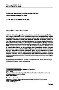
Figure 1: Two associated Legendre polynomials of degree n = 40 and order m = 33 and m = 36, showing the localization near the equator.

Polar optimization. High order spherical harmonics have their magnitude decrease exponentially when approaching the poles as shown in figure 1. Hence, the integral of expression 10 can be reduced to Z π−θ0mn m fm (θ)Pnm (cos θ) sin θ dθ (12) fn = θ0mn

where θ0mn ≥ 0 is a threshold below which Pnm is considered to be zero. Similarly, the synthesis of fm (θ) (eq. 7) is only needed for θ0mn ≤ θ ≤ π − θ0mn . SHTns uses a threshold θ0mn that does not depend on n, which leads to around 5% to 15% speed increase, depending on the desired accuracy and the truncation N . Cache optimizations. The precomputed coefficients Pnm (cos θj ) can be reordered and systematic zeros (due to polar optimization) can be stripped out, which leads to sensible speed increase. 3.2. On-the-fly algorithms and vectorization on the x86 platform It can be shown that Pnm (x) can be computed recursively by 2 m Pm (x) = am m 1−x m Pm+1 (x) Pnm (x)

= =


|m|/2

m am m+1 xPm (x) m m am n xPn−1 (x) + bn

(13) (14) (15)

m Pn−2 (x)

with am m

v u |m| u 1 Y 2k + 1 t = 4π 2k k=1

am n

=

r

4n2 − 1 n 2 − m2

bm n

=−

r

2n + 1 (n − 1)2 − m2 2n − 3 n 2 − m2

(16)

m The coefficients am n and bn do not depend on x, and can be easily precomputed and stored in an array of N (N +1) values. This has to be compared to the order N 3 values of Pnm (xj ), which are usually precomputed and stored in the spherical harmonic transforms implemented in numerical simulations. When N becomes very large, it is no longer possible to store Pnm (xj ) in memory (for N & 1023 nowadays) and on-the-fly algorithms (where the values of Pnm (xj ) are always computed from the recurrence relation when needed) are then the only possibility. Here, we would like to stress that even far from that storage limit, on-the-fly algorithm can be significantly faster thanks to vector capabilities of modern x86 processors. Most desktop and laptop computers, as well as

4

2.0

efficiency

1.5 1.0 0.5

on-the-fly 4-vector (AVX) on-the-fly 2-vector (SSE3)

0.0

precomputed matrices

102

N +1

103

Figure 2: Efficiency (N + 1)3 /(2tf ) of various algorithms, where t is the execution time and f the frequency of the Xeon E52680 CPU (2.7GHz). On-the-fly algorithms with two different vector sizes are compared with the algorithm using precomputed matrices. Note the influence of hardware vector size for on-the-fly algorithms (AVX vector pack 4 double precision floating point numbers where SSE3 vectors pack only 2). The efficiency of the algorithm based on precomputed matrices drops above N = 127 probably due to cache size limitations.

many high performance computing clusters, have support for Single-Instruction-Multiple-Data (SIMD) operations in double precision. The SSE2 instruction set is available since year 2000, and is currently supported by almost every PC, allowing to perform the same double precision arithmetic operations on a vector of 2 double precision numbers, effectively doubling the computing power. The recently introduced AVX instruction set increases the vector size to 4 double precision numbers. This means that the computation of Pnm (x) by the recursion relation 13 (which requires 3 multiplications and 1 addition) will become more and more efficient, as Pnm (x) can be computed for 2 or 4 values of x simultaneously. Practically speaking, computing Pnm (x) on-the-fly may be faster than loading pre-computed values from memory. Hence, as already pointed out by Dickson et al. [3], it is therefore very important to use the vector capabilities of modern processors to address their full computing power. Furthermore, when running multiple transforms on the different cores of a computer, the performance of on-the-fly transforms (which use less memory bandwidth) scales much better than algorithms with precomputed matrices, because the memory bandwidth is shared between cores. Superscalar architectures that do not have double-precision SIMD instructions but have many computation unit per core (like the POWER7 or SPARC64) could also benefit from on-the-fly transforms by saturating the many computation units with independent computations (at different x). Figure 2 shows the benefit of explicit vectorization of on-the-fly algorithms on an intel Xeon E5-2680 (Sandy Bridge architecture with AVX instruction set running at 2.7GHz) and compares on-the-fly algorithms with algorithms based on precomputed matrices. With the 4-vectors of AVX, the fastest algorithm is always on-the-fly, while for 2-vectors, the fastest algorithm uses precomputed matrices for N . 200. The efficiency drop for N = 2047 is due to the additional rescaling required to properly compute the recurrence relation at such high N with double-precision numbers. Runtime tuning. We have now two different available algorithm: one uses precomputed values for Pnm (x) and the other one computes them on-the-fly at each transform. The SHTns library compares the time taken by those algorithms (and variants) at startup and chooses the fastest, similarly to what the FFTW library[5] 5

N 63 127 255 511 1023 2047 4095

libpsht (1 thread) 1.05 ms 4.7 ms 27 ms 162 ms 850 ms 4.4 s 30.5 s

libpsht (12 threads) 5.0 ms 5.4 ms 8.5 ms 23.5 ms 125 ms 0.7 s 3.0 s

DH (fast) 1.1 ms 5.5 ms 21 ms 110 ms 600 ms NA NA

SHTns 0.09 ms 0.60 ms 4.2 ms 28 ms 216 ms 1.9 s NA

Table 1: Comparison of execution time for different SHT implementations. The numbers correspond to the average execution time for forward and backward scalar transform (including the FFT) on an Intel Xeon X5650 (2.67GHz) with 12 cores. The programs were compiled with gcc 4.4.5 and -O3 -march=native -ffast-math compilation options.

does. In the forthcoming years, AVX will become widely available, and the benefits of on-the-fly vectorized transforms will become even more important. 3.3. Performance comparisons Table 1 reports the timing measurements of two SHT libraries, compared to the optimized GaussLegendre implementation found in the SHTns library (this work). We compare with the Gauss-Legendre implementation of libpsht [9], a parallel spherical harmonic transform library targeting very large N , and with SpharmonicKit 2.7 (DH) which implements one of the Driscoll-Healy fast algorithms [6]. All the timings are for a complete SHT, which includes the Fast Fourier Transform. Note that the GaussLegendre algorithm is by far (a factor of order 2) the fastest algorithm of the libpsht library. Note also that SpharmonicKit is limited to N + 1 being a power of two, requires 2(N + 1) latitudinal colocation points, and crashed for N = 2047. The software library implementing the fast Legendre transform described in [7], libftsh, has also been tested, and found to be of comparable peformance to that of SpharmonicKit, although the comparison is not straightforward because libftsh did not include the Fourier Transform. Again, that fast library could not operate at N = 2047 because of memory limitations. Note finally that these measurements were performed on a machine that did not support the new AVX instruction set. In order to ease the comparison, we define the efficiency of the SHT by (N + 1)3 /(2tf p), where t is the execution time (reported in table 1), p the number of parallel threads (which is 12 for the parallel version of libpsht, and 1 otherwise) and f the frequency of the CPU (2.67GHz in this benchmark). This definition of efficiency takes into account the number of threads p, which is relevant for numerical simulations, where many SHT could be performed in parallel. For reference, we added the efficiency of the parallel algorithm with p set to 1, showing that even with 12 threads, libpsht performs better than SHTns only for N & 500. Note that (N + 1)3 /2 reflects the number of computation elements of a Gauss-Legendre algorithm (the number of modes (N + 1)(N + 2)/2 times the number of latitudinal points N + 1). An efficiency that does not depend on N corresponds to an algorithm with an execution time proportional to N 3 . The efficiency of the tested algorithms are displayed in figure 3. Not surprisingly, the Driscoll-Healy implementation has the largest slope, which means that its efficiency grows fastest with N , as expected for a fast algorithm. It also performs slightly better than libpsht for N ≥ 511. However, even for N = 1023 (the largest size that it can compute), it is still 2.8 times slower than the Gauss-Legendre algorithm implemented in SHTns. It is remarkable that SHTns achieves an efficiency very close to 1, meaning that almost one element per clock cycle is computed for N = 511 and N = 1023. Overall, SHTns is between two and ten times faster than the best alternative. We expect this gap to grow with the 4-vectors of the new AVX machines. 3.4. Accuracy One cannot write about an SHT implementation without addressing its accuracy. Here, the GaussLegendre quadrature ensures very good accuracy, at least on par with other high quality implementations. To quantify the error we start with random spherical harmonic coefficients Qm l with each real part and imaginary part between −1 and +1. After a backward and forward transform (with orthonormal spherical 6

efficiency

100

10-1 SHTns Gauss Driscoll-Healy libpsht 1T libpsht 12T

10-2

libpsht 12T (real time)

102

N +1

103

Figure 3: Efficiency (N + 1)3 /(2tf p) of the implementations from table 1, where t is the execution time, p the number of parallel threads and f the frequency of the Xeon X5650 CPU (2.67GHz) with 12 cores.

10-11 10

max error

-12

rms error

10-13 10-14 10-15

102

N +1

103

Figure 4: Accuracy of the on-the-fly Gauss-Legendre algorithm with the default polar optimization.

7

harmonics), we compare the resulting coefficients Rlm with the originals Qm l . We use two different error measurements: the maximum error is defined as ǫmax = max |Rlm − Qm l | l,m

while the root mean square (rms) error is defined as s X 2 2 ǫrms = |Rlm − Qm l | (N + 1)(N + 2) l,m

The error measurements for our on-the-fly Gauss-Legendre implementation with the default polar optimization and for various truncation degree N are shown on figure 4. 4. Conclusion and perspectives Despite the many fast spherical transform algorithms published, the few with a publicly available implementation are far from the performance of a carefully written Gauss-Legendre algorithm, as implemented in the SHTns library, even for quite large truncation (N = 1023). Explicitly vectorized on-the-fly algorithm seem to be able to unleash the computing power of nowadays and future computers, without suffering too much of memory bandwidth limitations. Such kind of algorithm, that uses more computing resources but less memory bandwidth, should also be efficient on GPU machines, and future work will involve an OpenCL implementation. Finally, by choosing at runtime the fastest available SHT algorithm, the SHTns library will most certainly deliver the fastest spherical transform to your platform. The versatile truncation, the various normalization conventions supported, as well as the scalar and vector transform routines available for C/C++, Fortran or Python, should suit most of the current and future needs in high performance computing. References References [1] Brun, A., Rempel, M., Apr. 2009. Large scale flows in the solar convection zone. Space Science Reviews 144 (1), 151–173. URL http://dx.doi.org/10.1007/s11214-008-9454-9 [2] Christensen, U. R., Aubert, J., Cardin, P., Dormy, E., Gibbons, S., Glatzmaier, G. A., Grote, E., Honkura, Y., Jones, C., Kono, M., Matsushima, M., Sakuraba, A., Takahashi, F., Tilgner, A., Wicht, J., Zhang, K., Dec. 2001. A numerical dynamo benchmark. Physics of The Earth and Planetary Interiors 128 (1-4), 25–34. URL http://dx.doi.org/10.1016/S0031-9201(01)00275-8 [3] Dickson, N. G., Karimi, K., Hamze, F., Jun. 2011. Importance of explicit vectorization for CPU and GPU software performance. Journal of Computational Physics 230 (13), 5383–5398. URL http://dx.doi.org/10.1016/j.jcp.2011.03.041 [4] Driscoll, J., Healy, D. M., June 1994. Computing fourier transforms and convolutions on the 2-sphere. Advances in Applied Mathematics 15 (2), 202–250. URL http://dx.doi.org/10.1006/aama.1994.1008 [5] Frigo, M., Johnson, S. G., Feb. 2005. The design and implementation of FFTW3. Proceedings of the IEEE 93 (2), 216–231. URL http://www.fftw.org/fftw-paper-ieee.pdf [6] Healy, D. M., Rockmore, D. N., Kostelec, P. J., Moore, S., July 2003. Ffts for the 2-sphere-improvements and variations. Journal of Fourier Analysis and Applications 9 (4), 341–385. URL http://dx.doi.org/10.1007/s00041-003-0018-9 [7] Mohlenkamp, M. J., 1999. A fast transform for spherical harmonics. The Journal of Fourier Analysis and Appications 5 (2/3). URL http://www.springerlink.com/content/n01v8q03m5584253/ [8] Potts, D., Steidl, G., Tasche, M., Oct. 1998. Fast algorithms for discrete polynomial transforms. Mathematics of Computation 67, 1577–1590. URL http://adsabs.harvard.edu/abs/1998MaCom..67.1577P [9] Reinecke, M., Feb. 2011. Libpsht – algorithms for efficient spherical harmonic transforms. Astronomy & Astrophysics 526, A108+. URL http://arxiv.org/abs/1010.2084

8

[10] Sakuraba, A., Feb. 1999. Effect of the inner core on the numerical solution of the magnetohydrodynamic dynamo. Physics of The Earth and Planetary Interiors 111 (1-2), 105–121. URL http://dx.doi.org/10.1016/S0031-9201(98)00150-2 [11] Sakuraba, A., Roberts, P. H., Oct. 2009. Generation of a strong magnetic field using uniform heat flux at the surface of the core. Nature Geoscience 2 (11), 802–805. URL http://dx.doi.org/10.1038/ngeo643 [12] Suda, R., Takami, M., 2002. A fast spherical harmonics transform algorithm. Mathematics of Computation 71 (238), 703–715. URL http://dx.doi.org/10.1090/S0025-5718-01-01386-2 [13] Temme, N. M., Aug. 2011. Gauss quadrature. In: Digital Library of Mathematical Functions (DLMF). National Institute of Standards and Technology (NIST), Ch. 3.5(v). URL http://dlmf.nist.gov/3.5.v [14] Tygert, M., Jan. 2008. Fast algorithms for spherical harmonic expansions, II. Journal of Computational Physics 227 (8), 4260–4279. URL http://dx.doi.org/10.1016/j.jcp.2007.12.019 [15] Wicht, J., Tilgner, A., May 2010. Theory and modeling of planetary dynamos. Space Science Reviews 152 (1), 501–542. URL http://dx.doi.org/10.1007/s11214-010-9638-y

9