Efficient Surface Reconstruction for Piecewise Smooth Objects Philipp Jenke and Michael Wand and Wolfgang Straßer email:
[email protected] [email protected] [email protected] WSI-2007-05 Dezember 2007
Graphisch-Interaktive Systeme Wilhelm-Schickard-Institut Universität Tübingen D-72076 Tübingen, Germany WWW: http://www.gris.uni-tuebingen.de
© WSI 2007 ISSN 0946-3852
Abstract In this report we present a new surface reconstruction technique from unstructured point clouds for piecewise smooth objects, such as scans of architectural and other man-made artifacts. The new technique operates in three conceptual steps: First, a set of basis functions is computed and a topology is established among these functions that respect sharp features using a RANSAC technique. Second, a linearized, statistically motivated optimization problem is solved employing this discretization. Lastly, an implicit function based meshing technique is employed to determine a clean, manifold mesh representation. The main benefit of our new proposal in comparison to previous work is its robustness and efficiency, which we examine by applying the algorithm to a set of synthetic and real-world benchmark data sets.
1
1
Introduction
Surface reconstruction from point clouds is meanwhile a classic topic in computer graphics. Reconstruction problems of this type arise in many areas of computer graphics, in particular when using 3D acquisition devices. In this paper, we examine an important special case, the reconstruction of piecewise smooth objects, i.e. objects that consist of smooth patches and crease lines of infinite curvature. This class of objects is of strong interest in practice because many man made objects, such as buildings or machine parts, are (at least approximately) of this structure. Typically, such objects can be represented using a fairly low complexity representation of smooth patches and boundary curves, while a high resolution point cloud is necessary to acquire the objects initially. In consequence, many traditional surface reconstruction techniques have high computational demands or even fail completely because of the high sampling requirements to represent the lines of first order singularity, which could be avoided by taking the special structure of the objects into account. Our new proposal consists of three building blocks: First, we derive a quadratic energy function for the reconstruction of smooth surfaces. The energy function is an approximation of the statistically motivated, non-linear formulation in [JWB+ 06, HAW07]. The energy function is discretized on a set of hierarchically adapted local quadratic basis functions that parametrize the shape space under consideration with a small number of coefficients and optimized by solving a simple sparse linear system. In a second step, we detect regions that are not well represented in this low-dimensional function space. We apply a RANSAC-based segmentation algorithm [FB87, SWK07] that creates multiple basis functions at sharp creases, breaks their topological connectivity accordingly and associates the original data points with the corresponding parts. Solving again for the global optimum of our energy function, we now obtain a piecewise smooth reconstruction with explicitly represented crease lines. These lines are well behaved, i.e. they themselves are piecewise smooth, as imposed by the smoothness constraints of the smooth patches. The third part of the algorithm then constructs a clean manifold mesh by blending and clipping implicit functions derived from the local basis functions. The output mesh is feature aware: The curvature information of the smooth patches is provided in terms of triangle normals and the crease lines are tessellated explicitly, appearing as a subset of the triangle edges. The main advantages of our new proposal are efficiency and robustness: Unlike previous statistical techniques [JWB+ 06,DTB06], the hierarchical adaptation of the basis functions and the linearized optimization technique allow for a very efficient reconstruction of smooth surface patches. In comparison to [HAW07], we adapt the support of our basis functions at sharp features rather than resorting to high resolution sampling, which drastically reduces computational costs in our application area. The approach is also robust: The RANSAC based fitting has been proven to reliably and robustly segment objects into smooth parts [SWK07]. Even in case the segmentation fails, it only affects the degrees of freedom present in the basis functions. The algorithm might miss a feature or overrepresent it, but this cannot have catastrophic consequences on the result. The remainder of the paper is structured as follows: Section 2 discusses the relation to previous techniques more in detail. Section 3 describes the recon2
struction algorithm and its components. We present results of our reconstruction system from synthetic and real-world architectural scans in Section 4 and evaluate the algorithm’s robustness under different noise conditions. Section 5 concludes the paper and points into possible future research directions.
2
Related Work
Surface reconstruction algorithms were pioneered by the work of Hoppe et al. [HDD+ 92], who estimate and unify point normals and then extract a triangle mesh via a reconstructed distance function. Amenta and colleagues [ABK98] approach the reconstruction problem from a computational geometry point of view, focusing on topology reconstruction. Carr et al. [CBC+ 01] use Radial Basis Functions to define the surface. The Moving Least Squares (MLS, [ABCO+ 03]) approach defines the surface as an invariant set of a projection operator, computed as a numerical optimization step on a locally constructed implicit function. Ohtake et al. [OBA+ 05] subdivide data points hierarchically using an octree. In the nodes, they represent the surface with quadratic functions which are blended together globally by weights summing to one (Multi-level Partition of Unity, MPU). In [KBH06], Kazhdan and colleagues describe surface reconstruction as a spatial Poisson problem. Recently, statistical data analysis and machine learning techniques, such as Diebel et al. [DTB06], who address the problem with Bayesian statistics, have gained some attention. Gal and colleagues [GSH+ 07] describe how to incorporate priors from a model database with additional information, as normals, to be used in the reconstruction process. Dinh and colleagues [DGS01] approximate the surface in regions containing sharp creases by employing anisotropic basis functions. The amount and directions of the anisotropy are detected automatically using PCA. However, the creases are only enhanced, while remaining smooth. Therefore, the extraction of a triangle mesh with sharp creases is not directly possible. Some approaches, as Reuter et al. [RJT+ 05], require for explicit user interaction to enrich the geometry of the input. Their projection operator accounts for high-frequency features building upon user-defined tags. The MPU approach [OBA+ 05] or the Algebraic Point Set Surfaces of Guennebaud and Gross [GG07] are able to represent sharp features if correct normals are given, which is not the case in scanned datasets. Estimated normals (e.g. using PCA), however, smooth out the singularities. Therefore, both approaches require manual tagging of points around features. In contrast, our system is able to infer exactly this information automatically and can therefore be used as a preprocessing for their data representations. Lipman and colleagues [LCOL07] build a system to handle sharp features upon the MLS projection scheme. They compute a singularity indicator field based on the error of the MLS approximation. During the MLS projection, a spline representation is used to segment smooth surface parts; then the MLS procedure is applied to each subset individually. The main drawback of their approach is that restricting the datasets to a single singularity within each influence radius significantly limits possible inputs (e.g. corners cannot be handled). Another MLS extension is proposed by Fleishman et al. [FCOS05]. In the projection process, points in a local influence radius are segmented into subsets
3
from smooth surface parts. For this segmentation, a robust forward search paradigm is applied to iteratively find reference planes with corresponding point subsets. The sets are filled with the points with the lowest residual from the plane model. With each new point a bivariate polynomial fit is updated until the residuals exceed a certain threshold. After this fitting process the point subset is removed and the algorithm is restarted on the remaining points. Its main problem is that the robust fitting of points is only applied to the reference planes, which makes the algorithm less stable in angled regions. We, in contrast, also fit curved primitives (sphere, cylinder). Additionally, they argue that the robust fit can be done efficiently by choosing random points spatially close to the first sample. However, in the presence of noise, this approach becomes instable compared to choosing points as far from each other as possible. Our RANSAC sampling draws the samples without such a constraint. Even tough this requires more sampling iterations, we perform computationally well, because we do not need to compute the fitting of a polynomial with each added sample. Jenke et al. [JWB+ 06] detect and optimize for sharp creases within a Bayesian framework. They assume that singularities in the reconstruction can be found in surface parts with high estimated curvature. Based on this assumption, they mark points as singularity points and handle them separately in the optimization process. The global nature of their optimization is problematic because the whole detection pipeline fails, if only a small part of a singularity is not detected correctly. Additionally, because of the high number of optimization parameters required (position of each point) and its non-linear nature, we are able to outperform [JWB+ 06] by an order of magnitude while maintaining the same reconstruction quality. This is mainly due to the adaptive subdivision of the input data and the powerful representation with polynomials representing large sets of data points. By disregarding the costly preprocessing (see Section 4) this ratio becomes even more severe. Especially the performance issue makes their approach impractical for large scenes. In [KBSS01], Kobbelt et al. describe an enriched distance function representation which employs more than one distance value at each point and can therefore be used for feature preserving triangulation via the Marching Cubes. They, however, also require for correct normals to detect sharp creases and – what is even more important – they already assume a triangle mesh as input, which is not available from scanning systems. Our data structure with an octree and basis functions is built upon the work of Huang and colleagues [HAW07] which, again, is similar to the MPU representation [OBA+ 05]. They address the problem of registering a set of scans to a global reference system. The surface reconstruction part is carried out on increasing detail levels. An important difference to our approach is that they do not allow for the reconstruction of sharp creases. In order to somehow overcome this limitation, a high sampling ratio is required, which is very often not available (e.g. see the outdoor scan in Section 4). For applications such as urban environment modeling, however, it is mandatory to provide triangle meshes with sharp features. A performance issue arises from the non-linear nature of their optimization routine and the fact that their octree structure is not used for adaptivity (optimization on same depth level for all nodes). This causes problems with ill-sampled and noisy regions while being unnecessarily expensive in planar regions.
4
3
Algorithm
(a) Input
(b) Preprocessing (c) Octree-Setup/ (d) Singularities/ (e) Triangulation Optimization Optimization
Figure 1: Reconstruction pipeline. Input: unstructured noisy point data – preprocessing: normal and curvature estimation at each point (brighter color corresponds to higher curvature) – creation of a spatial data structure and numerical optimization for basis function coefficients – segmentation along singularities via RANSAC and optimization – mesh extraction. As input to the algorithm, we expect an unstructured point cloud. We do not need surface normals in the data. In a preprocessing step, we estimate the curvature and a (rough) normal at each point. Then, we subdivide the data into an octree structure and setup our reconstruction representation in the leaf nodes. Therefore, in each leaf node, we estimate a local coordinate system and initialize a set of basis functions. We call this representation in the nodes Local Surface Function (LSF). It is uniquely identified (assuming fixed local coordinate frames) by the coefficients of the basis functions. This allows us to compute our reconstruction as the minimum of an energy function defined over these coefficients. For smooth surfaces, the set of coefficients minimizing the energy function already gives the final reconstruction. However, we use this solution as an intermediate step to detect leaf nodes as singularity candidates (exploiting assumptions on the noise level in the data). The powerful and robust RANSAC is used to segment such singularity candidates into smooth subsets and replace them by a new node for each such subset with an individual LSF representation. Then, the energy optimization procedure is applied again to obtain the final reconstruction. In a postprocessing phase we extract a triangle mesh.
3.1
Data Preprocessing
For the computation of a rough normal direction and the curvature, we need a local influence radius σ as a user-parameter. Algorithms are imaginable, though, to estimate it from the input (e.g. with Tensor Voting [MLT00] using different radii or by analyzing the eigenvalues of the covariance matrix of local neighborhoods). In order to estimate the normal direction, we follow [HDD+ 92] and estimate local reference frames T at each point via PCA using its σ-neighbors. Afterward, the normal directions are globally unified. Please note that close to feature lines, these normal directions differ from the exact surface normals of the original surface. We estimate the curvature at each data point di by fitting a 2nd -order polynomial in the least-squares sense to the σ-neighborhood: f (u, v) = c0 + c1 u + c2 v + c3 uv + c4 u2 + c5 v 2 5
From the Mean Curvature H and the Gaussian Curvature K [Opr97], H
=
K
=
(1+fv2 )fuu −2fu fv fuv +(1+fu2 )fvv 3
2(1+fu2 +fv2 ) 2 2 fuu fvv −fuv (1+fu2 +fv2 )2 ,
we compute a single curvature value as the maximum of the principle curvatures derived from H and K. We remove noise in the curvature field, if σ is small relative to the noise level in the data, by smoothing it with a Gaussian kernel. Finally, we estimate the noise standard deviation σnoise in the input data (assuming Gaussian noise) from the distances of the data points to their corresponding fitted polynomials.
3.2
Adaptive Surface Representation
Our surface representation is based on an octree data structure over the data. We stop the recursive subdivision process of the octree if a cell contains no more than navg points. navg is estimated as the average number of points in the σneighborhood in the data. In order to guarantee stability of the optimization, we make sure that the surface patch of each octree node contains at least a σ-ball of data points. If that is not the case, we add points from adjacent nodes (double assignment of points does not disturb our reconstruction process). In flat regions, this deep subdivision is not required (or not even desired). Therefore, we propose a detail-adaptive representation: for each leaf node, we determine the maximum curvature curvmax estimate of all data points contained. Inner nodes are then merged, if all√their child leaf nodes with bounding box size b and according diagonal d = 3b meet the criterion described in Figure 2 (the curvature curvmax implies a circle with radius r = curv1max , αmax = 30 degrees):
2 sin( αmax 2 ) b< √ 3curvmax
Figure 2: Detail-adaptive curvature criterion. For each leaf node containing data points, we then estimate a local coordinate system, consisting of two tangential directions and a normal, which is used to transform world-space points into the local coordinate system: T : (x, y, z) → (u, v, n). Again, we estimate these local coordinate systems via PCA and align them according to the data normals (Figure 3a). Please note that in contrast to [HAW07] we do not need to realign the coordinate systems, because they are based on the data points which remain fixed. The surface in each leaf node is then represented with NB basis functions bi and their corresponding coefficients
6
ci , parameterized via the tangential directions: f :R×R→R
f (u, v) =
NB X
ci bi (u, v)
i=1
We call the combination of a coordinate system with a set of locally defined basis functions a Local Surface Function (LSF).
(a) Hierarchical representation: the surface is represented in the leaf nodes of an octree structure via local coordinate systems (tangential directions: green, blue; normal direction: red) and a set of basis functions (green shaded disks).
(b) Consistency: we minimize the integral (light gray area) of difference between adjacent local surface functions fk and fl in two adjacent leaf node cells Ck and Cl over a border area Ak,l via Monte-Carlo integration (blue points).
(c) Singularities: noise level σnoise is exceeded in cell (left): detection of primitives and segmentation of data points from smooth surface parts; then, creation of new subnodes with individual coordinate frames Ti and LSFs fi .
Figure 3: Reconstruction algorithm: hierarchical octree representation, consistency energy term, singularity detection.
3.3
Optimization
Since the coordinate systems remain fixed, the reconstruction is completely described via the coefficient vector c of all coefficients ci in the LSFs. We assemble an energy function used to determine the optimal reconstruction result. We use the following notation: NC,k is the number of points in octree cell Ok . NO is the number of leaf nodes containing LSFs. The point p = (uj,k , vj,k , nj,k ) denotes the j th data point in cell Ok transformed into its local coordinate system. The combined reconstruction energy function consists of three components: a data fitting term Ef , a smoothness term Es and a consistency term between adjacent patches Ec . The combined energy functional is formulated as E = λf Ef + λs Es + λc Ec . Data Fitting: The first term enforces the reconstructed surface to lie close to the data points – the data fitting term Ef . We formulate it by penalizing the distances (height values) of the data points from the LSF: NC,k NB NO 1 X 1 X X Ef = (( ci,k bi (uj,k , vj,k )) − nj,k )2 . NO NC,k j=1 i=1 k=1
Smoothness: In order to control the smoothness of the surface, we introduce an additional term following the ideas of [JWB+ 06,HAW07]. We constrain 7
the curvature of the local surface functions by minimizing the integral of the sum of squared principal curvatures (integration domain is [−1, 1]2 , because the LSFs are scaled to this domain within each octree cell): Es =
NO Z 1 Z 1 1 X 2 2 2 fuu + 2fuv + fvv dvdu. NO −1 −1 k=1
Consistency: Neither the data fitting nor the smoothness term guarantee consistency between adjacent cells. In order to achieve this, we add an energy component minimizing the difference between the LSF between cell Ck and its counterparts in all adjacent cells (Cl ∈ N (Ck )) in the cell border regions (see Figure 3b): Ec =
NO 1 X 1 NO |N (Ck )| k=1
Z
X Cl ∈N (Ck )
(fk0 − fl0 )2 dA,
Ak,l
where fk0 and fl0 are the LSF of nodes k and l transformed into a common coordinate system, with an integration domain Ak,l in the same coordinate system. In practice, this integral is – depending on the choice of basis functions – mathematically involved to compute. Therefore, we use Monte-Carlo integration with |M | samples. This means that for the consistency between nodes k and l, we randomly choose points flm on the LSF of node l and corresponding closest points fkm on the LSF of node k to approximate the integral: NO 1 X 1 Ec = NO |N (Ck )| k=1
X Cl ∈N (Ck )
|M | 1 X m (f − flm )2 |M | m=1 k
In practice, this is solved by the same formulation as the data fitting term, replacing the data points by the consistency points. Our experiments showed that using 4 samples close to the touching plane of the two adjacent cell bounding boxes for each adjacent node is sufficient. Since the positions of the consistency points change with optimized LSFs, we update them several times in the solution process. In both the formulation of the fitting term and the consistency term, we only use the height values of the points in the coordinate system normal direction instead of the distance values from the surface functions. These height values, however, are an accurate approximation of the distance in our formulation, because the maximum curvature within each node is small due to the adaptive representation. Using the energy functions as described above, we are able to infer an optimization system of the form cAc + bc + d, where A ∈ RN ×N is a positive definite matrix and c is the solution vector (c, b ∈ RN ). The size of the matrix N = NB N0 computes from the product of the number of basis functions times the number of local surface cells. The scalar d does not influence the minimum solution. This is found by solving the linear system Ac = b, which can be done rather efficiently. Each of the three energy components builds a sparse matrix which again is important for fast optimization. In all our examples we used the weights λf = 1, λs = 0.1 and λc = 2.
8
3.4
Singularities
Implied by the data fitting energy Ef we get an estimate of the noise distribution in a node. Additionally, we can compute the probability p of the noise level in a node given the noise distribution σnoise as estimated in the preprocessing phase. If this probability p is low (in all our examples the criterion is: σnoise,node > 2σnoise , which means p < 0.05), we assume that this value results from an invalid LSF due to singularities in the cell – such cells are marked as singularity candidates. An obvious approach to handle them is to subdivide the singularity candidate leaf nodes into subsets belonging to smooth surface parts. The question is, how to find such a segmentation. A technique, which has already shown its stability for a similar problem [SWK07] is the RANSAC [FB87]. This randomized approach can be used to detect primitives in point sets; in our case planes, cylinders and spheres. The basic idea is rather simple: a set of sample points is randomly drawn from the point set. These points are used to dispense a guess for a primitive candidate (e.g. a plane is uniquely described by three sample points). Then, all other points in the point set are checked against the primitive guess. This is done by computing a score based on the distances of the points to the primitive guess (only points are considered with a distance smaller than 2σnoise ). The procedure is carried out nRAN SAC times (in our case nRAN SAC = 150) and the guess with the highest score is kept. All points that fit into the primitive (again based on σnoise ) are discarded from the point set and the segmentation algorithm is restarted on the reduced point set (Figure 3c). An important question is, if it is reasonable to assume that the leaf node subsets can be segmented using these three simple primitives. In our context it is reasonable, because only small parts of the surface are investigated that locally at least resemble such primitives (especially for ’man-made’-objects). Furthermore, the primitives in the segmentation are only used as a temporal approximation and not as the final reconstruction. In practice, we never experienced any problems with this assumption. However, it can theoretically not be avoided that a larger number of segments is found than required, since depending on the set of basis functions chosen, this representation could represent a bigger variety of surfaces than the primitives. After the primitives have been detected, a new LSF is created for each subset and used to replace the singularity candidate leaf node in the data structure. In order to improve the stability of both the primitive detection and the final reconstruction optimization, we slightly enlarge the set of points used in the detection phase by adding points from adjacent nodes. We also fill up the data points for each newly created LSF in order to meet the constraints applied when first creating the leaf nodes in the octree structure. After the processing of all leaf nodes in the octree, the optimization routine is applied again. The only modification required here, is that not all spatially adjacent nodes are used for the consistency energy term Ec , but only those corresponding to the same smooth surface part. We ensure this, by comparing the normals inferred from the LSFs of adjacent nodes at the intersection. If the scalar product falls below a threshold of 0.9, the nodes are not considered neighbors.
9
3.5
Triangulation
The final step in our reconstruction pipeline is the extraction of a triangle mesh. Therefore, we interpret our representation with LSFs as an implicit function by computing the distance from the surface. A very-well studied approach to extract a triangle mesh from an implicit function is the Marching Cubes (MC, [LC87]) algorithm. We apply it in each LSF node and obtain a triangle soup. Either the height of a point over the basis function representation is used or the closest point on the surface is computed using an iterative approach projecting the point onto the surface in surface normal direction (more accurate in bended regions). In order to get a consistent triangulation, we subdivide all leaf nodes to the same depth. A special handling, however, is required at singularity nodes. Here, we apply the marching cubes once for each subset-node and clip at planes implied by adjacent nodes, as similarly applied in [JWB+ 06]. The final mesh is then stitched together by snapping of spatially close vertices and a projection operator which projects mesh vertices onto the surface. In order to overcome some triangulation artifacts caused by the MC (e.g. thin triangles), standard mesh enhancement or simplification techniques can be applied on the resulting triangle mesh (we used a modified version of the Quadric Error Metrics [GH97] for Figure 1 and in the block example in the accompanying video). The space requirements for the MC triangles are never severe compared to the input point data, not even for large scenes, because even leaf nodes from the lowest depth level (used for the triangulation) cover a large number of data points. This effect could be improved even more by employing an adaptive triangulation scheme, e.g. as described in [KKDH07].
4
Results
We have implemented a system prototype in C++. We tested the functionality of the technique on a variety of datasets, both synthetic and acquired by scanning systems. For the timings in Table 1, we used an Intel Core 2, 2.13 GHz System with 2 GB of RAM. We used the same 2nd -order monomials as basis functions for the local surface representation as in the preprocessing stage. However, in order to use other basis functions one only has to implement an evaluation call for each basis function and to adjust the smoothness term Es . For the 2nd -order monomials in node k it computes to Es,k = 2c23,k + 4c24,k + 4c25,k . We use a Conjugate Gradient solver [She94] to solve the optimization problem. For performance reasons, we use an indexed octree referencing the actual points in a point set, speed up nearest-neighbor queries by keeping an additional knn-octree structure and cache neighbor relationships. Noise: We evaluated the stability of our representation in terms of robustness under different noise levels. The representation using patches, which cover a large number of data points, shows much better robustness compared to a point-based representation. The critical part of the process is the singularity detection part – to distinguish features from noise. We created a test dataset (Figure 4) and iteratively increased the noise level as long as the detection of the primitives was successful. The points which were detected as belonging to primitives were color-coded (plane: red; cylinder: green; sphere: blue). The left
10
part of Figure 4 shows the dataset corrupted with Gaussian noise of standard deviation of 0.5% of the bounding box size, the right with 0.75% of the bounding box size. With the lower noise level, the primitives are detected correctly leading to a correct reconstruction (lower row); however, with the higher noise level, the RANSAC method fails.
Figure 4: Stability under different noise levels: extraction of primitives (top row; planes: red, cylinders: green, spheres: blue). Successful reconstruction (left) and failed reconstruction (right, front corner). Synthetic data: We also tested our approach on well-known synthetic datasets: fandisk (Figure 5, top), block (Figure 5, middle) and bunny (Figure 5, bottom). The fandisk dataset is especially interesting because parts of the surface cannot be represented correctly by the three primitives plane, cylinder and sphere. However, the reconstruction (middle row) is still able to detect the sharp creases and the LSF-representation allows for a correct extraction of the triangle mesh. The block dataset was corrupted by Gaussian noise (standard deviation = 0.5% of bounding box size). This dataset is especially challenging in regions where the holes intersect, because there the angle between the intersecting surfaces is rather low. Still, our singularity detection approach successfully segments the leaf nodes. The reconstruction of the bunny datasets shows the adaptive subdivision and how well smooth parts of a surface are reconstructed. Real-word data: The most interesting datasets, are those coming from 11
Figure 5: Synthetic examples: fandisk (first row): input data, reconstruction with LSFs, triangulation; block (second row): input data, estimated curvature, reconstruction with LSFs, triangulation; smooth example: bunny (third row): estimated curvature, reconstruction with LSFs, triangulation. scanning systems. Figure 6 shows the scan of a building interior floor. This dataset was acquired by a mobile device assembling the scene from laser range scan slices with color information. The main issue with this dataset is that during the iterative scene assembly, registration errors occur which result in ’shadow’ walls parallel to the main surface. This obviously hurts our Gaussian noise assumption. However, it can be seen from the reconstruction result (Figure 6, top, right) and the detected singularity nodes (Figure 6, bottom, left) that our reconstruction system still handles the data correctly. We successfully extract a triangle mesh (bottom, middle) and create a textured model from the input data (bottom, right). Please note, that inaccurate color assignments are already inherent in the data. We also tested our system on an outdoor dataset (Figure 7) acquired by the same system. Here, the main challenge is that the point sampling is much less uniform and the dataset even contains some large holes (left image). The reconstruction is therefore somewhat coarser and regards high-frequency details in the data as noise (bushes, small boxes). The adaptive reconstruction of our approach can be observed in the middle image; the right image again shows a 12
textured rendering of the final reconstructed surface. In both example datasets some rough outliers resulting e.g. from windows or extremely specular surfaces were removed manually. Alternatively, it seems possible to use the singularity detection step for this purpose, which has not yet been exploited.
Figure 6: Real-world example: scan of a department floor: input data (top left), estimated curvature (top middle), reconstruction with local coordinate frames (top right), detected singularity nodes (bottom left), triangulation (bottom middle), textured triangle mesh (bottom right).
Figure 7: Real-world example: scan of an outdoor environment: input data (left), reconstructed LSFs (middle), textured triangle mesh (right). Please note, that the complete reconstruction is based on very few and simple basis functions. Timings: Table 1 lists the timing results for the examples in the paper. It becomes obvious that a significant amount of computation time is required for the preprocessing. Since we only need a rough estimate for the curvature and only few consistent normals in the octree creation process, the preprocessing could be sped up significantly. The different timings in the singularity detection process result from different sizes of the local point sets used to detect the primitives and from the different number of singularity candidates. The bunny example is computationally more expensive due to its large number of LSFs resulting from the surface details. The timings imply that the reconstruction complexity is roughly linear with the number of input points, however this strongly depends on properties of the data such as sampling spacing and number/size of singularities.
13
Model/
Prepro-
Octree/
Optimi-
Singu-
Trian-
#points
cessing
#LSF-nodes
zation
larities
gulation
carved object/192k
22.1s
1.7s/1604
5.3s
1.9s
0.3s
fandisk/400k
39.7s
3.5s/1742
9.95s
9.3s
1.4s
block/200k
21.4s
1.6s/715
7.51s
32.6s
0.5s
bunny/1000k
149.3s
12.4s/5712
45.8s
-
9.3s
floor/1140k
160.0s
8.9s/880
16.0s
16.5s
0.6s
outdoor/177k
40.8s
1.6s/450
5.2s
13.0s
0.6s
Table 1: Timing results in seconds.
5
Conclusions and Future Work
In this paper we presented a novel method for the reconstruction of a surface representation from unstructured point geometry information. We preserve and enhance sharp creases in the input data and exploit this information in the final triangulation step. We use a hierarchical subdivision of the scene and represent the surface with a coordinate system and a set of basis functions in the leaf nodes (LSF). In order to handle sharp creases, we automatically detect nodes which possibly contain a singularity and segment the smooth surface parts using the RANSAC principle. In order to find the coefficients of the LSFs and therefore our final reconstruction, we assemble an energy function consisting of a data fitting, a smoothness and a consistency term, which we optimize by solving a linear system. We specifically address datasets of man-made objects with partly simple (close to planar) parts and sharp features. Especially, in terms of performance and robustness, our method beats existing approaches. A typical problem with an octree representation results from discretization artifacts. If a noisy surface is close to the touching plane of two adjacent cells, two parallel surface parts could result in the reconstruction. In future work, we would like to investigate if one can overcome this limitation by breaking up the octree structure and use a representation more adaptive to the data. Also, we would like to consider the problem in a more statistical way and investigate other possible priors which – especially for ’man-made’ datasets with many symmetries – could allow for a more faithful reconstruction of datasets with even finer structures.
References [ABCO+ 03] Marc Alexa, Johannes Behr, Daniel Cohen-Or, Shachar Fleishman, David Levin, and Claudio T. Silva. Computing and rendering point set surfaces. IEEE Transactions on Visualization and Computer Graphics, 9:3–15, 2003. [ABK98]
Nina Amenta, Marshall Bern, and Manolis Kamvysselis. A new voronoi-based surface reconstruction algorithm. In Proceedings SIGGRAPH ’98, 1998.
[CBC+ 01]
J. C. Carr, R. K. Beatson, J. B. Cherrie, T. J. Mitchell, W. R. Fright, B. C. McCallum, and T. R. Evans. Reconstruction and
14
representation of 3d objects with radial basis functions. In Proceedings SIGGRAPH ’01, 2001. [DGS01]
H. Q. Dinh, G.Turk, and G. Slabaugh. Reconstructing surfaces using anisotropic basis functions. In Proceedings International Conference on Computer Vision (ICCV ’01), 2001.
[DTB06]
James R. Diebel, Sebastian Thrun, and Michael Bruenig. A bayesian method for probable surface reconstruction and decimation. ACM Transactions on Graphics, 25:39–59, 2006.
[FB87]
Martin A. Fischler and Robert C. Bolles. Random sample consensus: A paradigm for model fitting with applications to image analysis and automated cartography. Readings in Computer Vision: Issues, Problems, Principles and Paradigms, 24:726–740, 1987.
[FCOS05]
Shachar Fleishman, Daniel Cohen-Or, and Claudio T. Silva. Robust moving least-squares fitting with sharp features. In Proceedings SIGGRAPH ’05, 2005.
[GG07]
Gaël Guennebaud and Markus Gross. Algebraic point set surfaces. In Proceedings SIGGRAPH ’07, 2007.
[GH97]
Michael Garland and Paul S. Heckbert. Surface simplification using quadric error metrics. In Proceedings SIGGRAPH ’97, 1997.
[GSH+ 07]
Ran Gal, Ariel Shamir, Tal Hassner, Mark Pauly, and Daniel Cohen-Or. Surface reconstruction using local shape priors. In Proceedings Symposium on Geometry Processing (SGP ’07), 2007.
[HAW07]
Q. Huang, B. Adams, and M. Wand. Bayesian surface reconstruction via iterative scan alignment to an optimized prototype. In Proceedings Symposium on Geometry Processing (SGP ’07), 2007.
[HDD+ 92]
Hugues Hoppe, Tony DeRose, Tom Duchamp, John McDonald, and Werner Stuetzle. Surface reconstruction from unorganized points. In Proceedings SIGGRAPH ’92, 1992.
[JWB+ 06]
P. Jenke, M. Wand, M. Bokeloh, A. Schilling, and W. Straßer. Bayesian point cloud reconstruction. Computer Graphics Forum (Proceedings EG ’06), 25(3):379–388, 2006.
[KBH06]
M. Kazhdan, M. Bolitho, and H. Hoppe. Poisson surface reconstruction. In Proceedings Symposium on Geometry Processing (SGP ’06), 2006.
[KBSS01]
Leif P. Kobbelt, Mario Botsch, Ulrich Schwanecke, and Hans-Peter Seidel. Feature sensitive surface extraction from volume data. In Proceedings SIGGRAPH ’01, 2001.
[KKDH07]
Michael Kazhdan, Allison Klein, Ketan Dalal, and Hugues Hoppe. Unconstrained isosurface extraction on arbitrary octrees. In Proceedings Symposium on Geometry Processing (SGP ’07), 2007.
15
[LC87]
William E. Lorensen and Harvey E. Cline. Marching cubes: A high resolution 3d surface construction algorithm. In Proceedings SIGGRAPH ’87, 1987.
[LCOL07]
Yaron Lipman, Daniel Cohen-Or, and David Levin. Datadependent mls for faithful surface approximation. In Proceedings Symposium on Geometry Processing (SGP ’07), 2007.
[MLT00]
G. Medioni, Mi-Suen Lee, and Chi-Keung Tang. A Computational Framework for Segmentation and Grouping. Elsevier, 2000.
[OBA+ 05]
Yutaka Ohtake, Alexander Belyaev, Marc Alexa, Greg Turk, and Hans-Peter Seidel. Multi-level partition of unity implicits. In Proceedings SIGGRAPH ’05, 2005.
[Opr97]
John Oprea. Differential Geometry and its Applications. PrenticeHall, Inc., 1997.
[RJT+ 05]
P. Reuter, P. Joyot, J. Truntzler, T. Boubekeur, and C. Schlick. Surface reconstruction with enriched reproducing kernel particle approximation. In Proceedings Point-Based Graphics (PBG ’05), 2005.
[She94]
Jonathan R Shewchuk. An introduction to the conjugate gradient method without the agonizing pain. Technical report, Carnegie Mellon University, 1994.
[SWK07]
R. Schnabel, R. Wahl, and R. Klein. Efficient ransac for pointcloud shape detection. Computer Graphics Forum, 26:214–226, 2007.
16