Piecewise-Smooth Support Vector Machine for Classification

Hindawi Publishing Corporation Mathematical Problems in Engineering Volume 2013, Article ID 135149, 7 pages http://dx.doi.org/10.1155/2013/135149

Research Article Piecewise-Smooth Support Vector Machine for Classification Qing Wu and Wenqing Wang School of Automation, Xi’an University of Posts and Telecommunications, Xi’an 710121, China Correspondence should be addressed to Qing Wu; [email protected] Received 18 November 2012; Revised 12 March 2013; Accepted 13 March 2013 Academic Editor: Jun Zhao Copyright © 2013 Q. Wu and W. Wang. This is an open access article distributed under the Creative Commons Attribution License, which permits unrestricted use, distribution, and reproduction in any medium, provided the original work is properly cited. Support vector machine (SVM) has been applied very successfully in a variety of classification systems. We attempt to solve the primal programming problems of SVM by converting them into smooth unconstrained minimization problems. In this paper, a new twice continuously differentiable piecewise-smooth function is proposed to approximate the plus function, and it issues a piecewise-smooth support vector machine (PWSSVM). The novel method can efficiently handle large-scale and high dimensional problems. The theoretical analysis demonstrates its advantages in efficiency and precision over other smooth functions. PWSSVM is solved using the fast Newton-Armijo algorithm. Experimental results are given to show the training speed and classification performance of our approach.

1. Introduction In the last several years, support vector machine (SVM) has become one of the most promising learning machines because of its high generalization performance and wide applicability for classification, forecasting, and estimation in small-sample cases [1–6]. In addition, SVMs have surpassed the performance of artificial neural networks in many areas such as text categorization, speech recognition, and bioinformatics [7–11]. Basically, the main idea behind SVM is the construction of an optimal hyper plane, which has been used widely in classification [5, 8–16]. It can be formulated into an unconstrained optimization problem [17–21], but the objective function is nonsmooth. To overcome this disadvantage, Lee and Mangasarian used the integral of the sigmoid function to get a smooth SVM(SSVM) model in 2001 [17]. It is a very important and significant result to SVM since many famous algorithms can be used to solve it. In 2005, Yuan et al. proposed two polynomial functions, namely, the smooth quadratic polynomial function and the smooth forth polynomial function, and got QPSSVM and FPSSVM models [20, 21]. Xiong et al. derived an important recursive formula and a new class of smoothing functions using the technique of interpolation functions in [20]. In 2007, Yuan et al. used a three-order spline function to smooth the objective function

of unconstrained optimization problem of SVM and obtained TSSVM model [21]. However, the efficiency or the precision of the algorithms was limited. A natural problem is whether there is another smooth function to get a more efficient smooth SVM than existing works. In this paper, we introduce a piecewise function to smooth SVM and obtain a novel piecewise smooth support vector machine (PWSSVM). Theoretical analyses show that approximation accuracy of the piecewise smooth function to the plus function is higher than the available. Rough set theory is used to prove the global convergence of PWSSVM and the upper bound of convergence is proposed. The fast Newton-Armijo algorithm [22, 23] is employed to train the PWSSVM. Our new method is implemented in batches and can efficiently handle large-scale and high dimensional problems. Numerical experiments confirm the theoretical results and demonstrate that PWSSVM is more effective than the previous smooth support vector machine models. The paper is organized as follows. In Section 2, we state the pattern classification and describe the PWSSVM. The approximation performance of smooth functions to the plus function is compared in Section 3. The convergence performance of PWSSVM is given in Section 4. The NewtonArmijo algorithm is applied to train PWSSVM in Section 5. Section 6 shows numerical comparisons. Finally, a brief conclusion of this paper is made.

2

Mathematical Problems in Engineering

In this paper, unless otherwise stated, all vectors are column vectors. For a vector 𝑥 in the 𝑛-dimensional real space 𝑅𝑛 , the plus function 𝑥+ is defined as (𝑥+ )𝑖 = max (0, 𝑥𝑖 ), 𝑖 = 1, . . . , 𝑛. The scalar (inner) product of two vectors 𝑥, 𝑦 in the 𝑛-dimensional real space will be denoted by 𝑥 ⋅ 𝑦 and the 𝑝-norm will be denoted by ‖ ⋅ ‖𝑝 . For a matrix 𝐴 ∈ 𝑅𝑚×𝑛 , 𝐴 𝑖 is the 𝑖th row of 𝐴 which is a row vector in 𝑅𝑛 . A column vector of ones of 𝑛 dimension will be denoted by 𝑒. If 𝜑 is a real valued function defined in the 𝑛-dimensional real space 𝑅𝑛 , the gradient of 𝜑 is denoted by ∇𝜑(𝑥) which is a row vector in 𝑅𝑛 and 𝑛 × 𝑛 the Hessian matrix of 𝜑 at 𝑥 is denoted by ∇2 𝜑(𝑥).

2. Piecewise-Smooth Support Vector Machine In this paper, let us consider a binary classification problem with 𝑚 training samples in the 𝑛-dimensional real space 𝑅𝑛 . It is represented by the 𝑚 × 𝑛 matrix 𝐴, according to membership of each point 𝐴 𝑖 in the class 1 or −1 as specified by a given 𝑚 × 𝑚 diagonal matrix 𝐷 with 1 or −1 along its diagonal. For this problem, the standard SVM with a linear kernel is given by the following quadratic program with parameter 𝜐 > 0 min

(𝑤,𝛾,𝑦)∈𝑅𝑛+1+𝑚

s.t.

1 𝜐𝑒Τ 𝑦 + 𝑤Τ 𝑤 2

(1)

𝐷 (𝐴𝑤 − 𝑒𝛾) + 𝑦 ≥ 𝑒 𝑦 ≥ 0,

where 𝑒 is a vector of ones, 𝑤 is the normal to the bounding plane, and 𝑏 is the distance of the bounding plane to the origin. The linear separating plane is defined as follows: 𝑃 = {𝑥𝑖 | 𝑥𝑖 ∈ 𝑅𝑛 , 𝑤Τ 𝑥𝑖 = 𝑏} .

(2)

The first term in the objective function of (1) is the 1-norm of the slack variable 𝑦 with weight 𝜐. Replace the first term with the 2-norm vector 𝑦. Add (1/2)𝛾Τ 𝛾 to the objective function which induces strong convexity but has little or no effect on the problem. SVM model is replaced by the following problem: min𝑛+1+𝑚

(𝑤,𝛾,𝑦)∈𝑅

s.t.

𝜐 Τ 1 𝑦 𝑦 + (𝑤Τ 𝑤 + 𝛾Τ 𝛾) 2 2

(3)

𝐷 (𝐴𝑤 − 𝑒𝛾) + 𝑦 ≥ 𝑒 𝑦 ≥ 0.

Let 𝑦 = (𝑒 − 𝐷(𝐴𝑤 − 𝑒𝛾))+ , where (⋅)+ replaces negative components of a vector by zeros, then we can convert the SVM problem (3) into the following unconstrained optimization problem: min

(𝑤,𝛾)∈𝑅𝑛+1

1 󵄩󵄩 󵄩2 1 𝜐󵄩(𝑒 − 𝐷 (𝐴𝑤 − 𝑒𝛾))+ 󵄩󵄩󵄩 + (𝑤Τ 𝑤 + 𝛾Τ 𝛾) . (4) 2 󵄩 2

This is a strongly convex minimization problem and it has a unique solution. Let max {0, 𝑥} = 𝑥+ . The function (𝑥)+ is a continuous but nonsmooth function. Therefore, many optimization algorithms based on derivative and gradient cannot solve the problem (4) directly.

In 2001, Lee and Mangasarian [17] employed the integral of the sigmoid function 𝑝(𝑥, 𝑘) to approximate the nondifferentiable function 𝑥+ as follows: 1 (5) 𝑘 > 0, log (1 + 𝜀−𝑘𝑥 ) , 𝑘 where 𝜀 is the base of natural logarithm and 𝑘 is a smoothing parameter. They got the SSVM model. In 2005, Yuan et al. [18] presented two polynomial functions as follows: 1 𝑥, 𝑥≥ , { { { 𝑘 { { { {𝑘 1 1 1 1 𝑞 (𝑥, 𝑘) = { 𝑥2 + 𝑥 + , − < 𝑥 < , 𝑘 > 0, { 4 2 4𝑘 𝑘 𝑘 { { { { 1 { 0, 𝑥≤− , { 𝑘 𝑝 (𝑥, 𝑘) = 𝑥 +

1 𝑥, 𝑥≥ , { { { 𝑘 { { { { 1 1 1 ℎ (𝑥, 𝑘) = {− (𝑘𝑥 + 1)3 (𝑘𝑥 − 3) , − < 𝑥 < , 𝑘 > 0, { 16𝑘 𝑘 𝑘 { { { { 1 { 0, 𝑥≤− . { 𝑘 (6) Using the above smooth functions to proximate plus function 𝑥+ , they got two smooth polynomial support vector machine models (FPSSVM and QPSSVM). The authors also showed that FPSSVM and QPSSVM were more effective than SSVM in [18]. In 2007, Yuan et al. [21] presented a three-order spline function as follows: 1 0, 𝑥 . {𝑥, 𝑘 (7) They used the smooth function 𝑇(𝑥, 𝑘) to approach the plus function and got a new smooth SVM model TSSVM. However, the efficiency or the precision of these algorithms above was limited. In this paper, we propose a novel smooth function 𝜑(𝑥, 𝑘) with smoothing parameter 𝑘 > 0 to approximate to the function 𝑥+ as follows: 1 0, 𝑥 . { 3𝑘


3

The first- and second-order derivatives of 𝜑(𝑥, 𝑘) are 0, { { { { { { { { 9 2 1 2 { { + 𝑘 (𝑥 ), { {2 3𝑘 ∇𝜑 (𝑥, 𝑘) = { 2 { 9 1 { { { 1 − 𝑘2 ( − 𝑥) , { { 2 3𝑘 { { { { { 1, { { 0, { { { { { { { 1 { { 9𝑘2 (𝑥 + ) , { { 3𝑘 ∇2 𝜑 (𝑥, 𝑘) = { { 1 2 { { 9𝑘 ( − 𝑥) , { { 3𝑘 { { { { { {0, {

𝑥 , 3𝑘

(3) for any 𝑥 ∈ 𝑅, 𝑇(𝑥, 𝑘)2 − 𝑥+2 ≤ 1/24𝑘2 .

−

𝑥 . 3𝑘

−

The solution of the problem (3) can be obtained by solving the following smooth unconstrained optimization problem with the smoothing parameter 𝑘 approaching infinity as min Φ𝑘 (𝑤, 𝛾) =

(𝑤,𝛾)∈𝑅𝑛+1

1 󵄩󵄩 󵄩2 𝜐󵄩𝜑 (𝑒 − 𝐷 (𝐴𝑤 − 𝑒𝛾) , 𝑘)󵄩󵄩󵄩 2 󵄩 1 + (𝑤Τ 𝑤 + 𝛾Τ 𝛾) . 2

(10)

Thus, we develop a new smooth approximation for problem (3).

In this section, we will compare the approximation performance of smooth functions to plus function. Lemma 1 (see [17]). 𝑝(𝑥, 𝑘) is defined as the integral of the sigmoid function in [17], and 𝑥+ is the plus function. The following conclusions can be obtained: (1) 𝑝(𝑥, 𝑘) is arbitrary rank smooth about 𝑥; (2) 𝑝(𝑥, 𝑘) ≥ 𝑥+ ;

Lemma 2 (see [18]). 𝑞(𝑥, 𝑘) and ℎ(𝑥, 𝑘) are defined as (6), and 𝑥+ is plus function. We can obtain the following conclusions: (1) 𝑞(𝑥, 𝑘) is one rank smooth about 𝑥, and ℎ(𝑥, 𝑘) is twice rank smooth about 𝑥; (2) 𝑞(𝑥, 𝑘) ≥ 𝑥+ and ℎ(𝑥, 𝑘) ≥ 𝑥+ ; (3) for any 𝑥 ∈ 𝑅, 𝑞(𝑥, 𝑘) − 𝑥+2 ≤ 1/19𝑘2 .

2

2

3 3 1 𝑠 (𝑥) = 𝜑(𝑥, 𝑘)2 − 𝑥+2 = (𝑥 + 𝑘2 ( − 𝑥) ) − 𝑥2 2 3𝑘

(11)

In order to obtain the result, making the variable substitution 𝑡 = 𝑘𝑥 (obviously 𝑡 ∈ (0, 1/3)), then we have 𝑠(𝑡) = (3/ 𝑘2 )[(3/4)(𝑡 − (1/3))6 − 𝑡(𝑡 − (1/3))3 ]. For 𝑡 ∈ (0, 1/3), the maximum point of 𝑠(𝑡) is 𝑡 = 0.0605 and 𝑠(𝑡) = 𝜑2 (𝑥, 𝑘) − (𝑥)2+ ≤ 𝑔(0.0605) ≈ 0.0046/𝑘2 ≤ 1/216𝑘2 . In conclusion, we have 𝜑(𝑥, 𝑘)2 − 𝑥+2 ≤ 1/216𝑘2 . Theorem 5. Let 𝜌 = 1/𝑘, and 𝑘 > 0. Consider the following.

(3) for 𝜌 > 0, |𝑥| < 𝜌, 𝑝(𝑥, 𝑘)2 − 𝑥+2 ≤ (log 2/𝑘)2 + (2𝜌/ 𝑘) log 2.

𝑥+2

Proof. (1) According to the formulas (8) and (9), one can easily obtain the results in (1). (2) In the following, we verify the fact 𝜑(𝑥, 𝑘) ≥ (𝑥)+ ≥ 0. (i) The equation 𝜑(𝑥, 𝑘) = (𝑥)+ holds while 𝑥 ∈ (−∞, −(1/ 3𝑘)) ∪ (1/3𝑘, ∞). (ii) Since 𝜑(𝑥, 𝑘) is a monotone increasing function, we have the following result 𝜑(𝑥, 𝑘) − (𝑥)+ = 𝜑(𝑥, 𝑘) ≥ 𝜑(−(1/3𝑘), 𝑘) = 0 while 𝑥 ∈ [−(1/3𝑘), 0). (iii) For 𝑥 ∈ [0, 1/3𝑘], we have 𝜑(𝑥, 𝑘) − (𝑥)+ = (3/2)𝑘2 (1/3𝑘 − 𝑥)3 ≥ 0. Hence, we have the conclusion 𝜑(𝑥, 𝑘) ≥ (𝑥)+ ≥ 0. (3) For 𝑥 ∈ (−∞, −(1/3𝑘)) ∪ (1/3𝑘, ∞), 𝜑(𝑥, 𝑘)2 − 𝑥+2 = 0, the inequality in conclusion (3) is satisfied naturally. For −(1/3𝑘) ≤ 𝑥 ≤ 0, since 𝑥+ = 0, 𝜑(𝑥, 𝑘)2 − 𝑥+2 = 𝜑(𝑥, 2 𝑘) . Because 𝜑(𝑥, 𝑘) is positive value, continuous, and increasing function for −(1/3𝑘) ≤ 𝑥 ≤ 0, we have 𝜑(𝑥, 𝑘)2 ≤ 𝜑(0, 𝑘)2 = 1/324𝑘2 ≤ 1/216𝑘2 . For 0 < 𝑥 ≤ 1/3𝑘, let

9 1 6 1 3 = 𝑘4 (𝑥 − ) − 3𝑘2 𝑥(𝑥 − ) . 4 3𝑘 3𝑘

3. Approximation Performance Analysis of Smooth Functions

2

(3) for any 𝑥 ∈ 𝑅, then 𝜑(𝑥, 𝑘)2 − 𝑥+2 ≤ 1/216𝑘2 .

(1) If the smooth function is defined as (5), then by Lemma 1, we have 𝑝(𝑥, 𝑘)2 − 𝑥+2 ≤ (

log 2 2 2𝜌 ) + log 2 𝑘 𝑘

1 1 = (log 2 + 2 log 2) 2 ≈ 0.6927 2 . 𝑘 𝑘

(2) If the smooth functions are defined as (6), by Lemma 2,

2

≤ 1/11𝑘 and ℎ(𝑥, 𝑘) −

Lemma 3 (see [19]). 𝑇(𝑥, 𝑘) is defined as (7), and 𝑥+ is plus function. The following results are easily obtained:

(12)

2

𝑞(𝑥, 𝑘)2 − 𝑥+2 ≤ 2

ℎ(𝑥, 𝑘) −

𝑥+2

1 1 ≈ 0.0909 2 , 11𝑘2 𝑘

1 1 ≤ ≈ 0.0526 2 . 2 19𝑘 𝑘

(13)

4

Mathematical Problems in Engineering (3) If the smooth function is defined as (7), by Lemma 3, 𝑇(𝑥, 𝑘)2 − 𝑥+2 ≤

1 1 ≈ 0.0417 2 . 2 24𝑘 𝑘

1 1 ≈ 0.0046 2 . 2 216𝑘 𝑘

0.12

(14)

0.1

(4) If the smooth function is defined as (8), by Theorem 4, 𝜑(𝑥, 𝑘)2 − 𝑥+2 ≤

0.14

(15)

𝑦

0.08 0.06 0.04

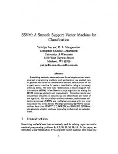
Theorem 5 shows that the proposed piecewise smooth function 𝜑(𝑥, 𝑘) achieves the best degree of approximation to the plus function 𝑥+ . When 𝑘 is fixed, it is easy to obtain the different smooth capability of the above smooth functions. The smooth performance comparison is given in Figure 1, where we set the smooth parameter 𝑘 = 10 and 𝜌 = 1/𝑘.

4. Convergence Performance of PWSSVM In this section, the convergence of PWSSVM will be presented. By using rough set theory, we prove that the solution of PWSSVM can closely approximate the optimal solution of the original model (4) when 𝑘 goes to infinity. Furthermore, a formula for computing the upper bound of convergence is deduced. Theorem 6. Let 𝐴 ∈ 𝑅𝑚×𝑛 and 𝑏 ∈ 𝑅𝑚×1 . Define the realvalued functions in the 𝑛-dimensional real space 𝑅𝑛 as follows: 1󵄩 󵄩2 1 𝑓 (𝑥) = 󵄩󵄩󵄩(𝐴𝑥 − 𝑏)+ 󵄩󵄩󵄩2 + ‖𝑥‖22 , 2 2 1󵄩 󵄩2 1 𝑔 (𝑥, 𝑘) = 󵄩󵄩󵄩𝜑 (𝐴𝑥 − 𝑏, 𝑘)󵄩󵄩󵄩2 + ‖𝑥‖22 , 2 2

(16)

(1) 𝑓(𝑥) and 𝑔(𝑥, 𝑘) are strongly convex functions; (2) there exists a unique solution 𝑥∗ to min𝑥∈𝑅𝑛 𝑓(𝑥), and a unique solution 𝑥𝑘∗ to min𝑥∈𝑅𝑛 𝑔(𝑥, 𝑘); (3) for any 𝑘 > 0, 𝑥𝑘∗ and 𝑥∗ satisfy the following condition:

(4)

lim𝑘 → ∞ ‖𝑥𝑘∗

0 −0.1 −0.08 −0.06 −0.04 −0.02

0 𝑥

0.02 0.04 0.06 0.08

0.1

Plus function Integral of sigmoid function Quadratic polynomial function Forth polynomial function Three-order spline function Piecewise function

Figure 1: Comparison of approximation performance of smooth functions (𝑘 = 10).

(3) By using the first order optimization condition and considering convex property of 𝑓(𝑥) and 𝑔(𝑥, 𝑘), we have 1󵄩 󵄩2 𝑓 (𝑥𝑘∗ ) − 𝑓 (𝑥∗ ) ≥ ∇𝑓 (𝑥∗ ) (𝑥𝑘∗ − 𝑥∗ ) + 󵄩󵄩󵄩𝑥𝑘∗ − 𝑥∗ 󵄩󵄩󵄩2 2 1󵄩 󵄩2 = 󵄩󵄩󵄩𝑥𝑘∗ − 𝑥∗ 󵄩󵄩󵄩2 , 2

where 𝜑(⋅) is defined in (8), 𝑘 > 0. Then we have the following results:

𝑚 󵄩󵄩 ∗ ∗ 󵄩2 ; 󵄩󵄩𝑥𝑘 − 𝑥 󵄩󵄩󵄩 ≤ 432𝑘2

0.02

(17)

∗

− 𝑥 ‖ = 0.

Proof. (1) For any 𝑘 > 0, 𝑓(𝑥) and 𝑔(𝑥, 𝑘) are strongly convex functions because ‖ ⋅ ‖2 is strong convex function. (2) Let 𝐿 V (𝑓(𝑥)) be the level set of 𝑓(𝑥) and let 𝐿 V (𝑔(𝑥, 𝑘)) be the level set of 𝑔(𝑥, 𝑘). Since 𝑥+ ≤ 𝜑(𝑥, 𝑘), it is easy to obtain 𝐿 V (𝑔(𝑥, 𝑘)) ⊂ 𝐿 V (𝑓(𝑥)) ⊂ {𝑥 | ‖𝑥‖22 ≤ 2V}. Therefore, 𝐿 V (𝑓(𝑥)) and 𝐿 V (𝑔(𝑥, 𝑘)) are compact subsets in 𝑅𝑛 . Using the strong convexity property of 𝑓(𝑥) and 𝑔(𝑥, 𝑘) for 𝑘 > 0, there is a unique solution to min𝑥∈𝑅𝑛 𝑓(𝑥) and min𝑥∈𝑅𝑛 𝑔(𝑥, 𝑘), respectively.

1󵄩 󵄩2 𝑔 (𝑥∗ , 𝑘) − 𝑔 (𝑥𝑘∗ , 𝑘) ≥ ∇𝑔 (𝑥𝑘∗ , 𝑘) (𝑥∗ − 𝑥𝑘∗ ) + 󵄩󵄩󵄩𝑥𝑘∗ − 𝑥∗ 󵄩󵄩󵄩2 2 1󵄩 󵄩2 = 󵄩󵄩󵄩𝑥𝑘∗ − 𝑥∗ 󵄩󵄩󵄩2 . 2

(18)

Add the two formulas above and notice that 𝜑(𝑥, 𝑘) ≥ 𝑥+ , and then we have 󵄩󵄩 ∗ ∗ 󵄩2 ∗ ∗ ∗ ∗ 󵄩󵄩𝑥𝑘 − 𝑥 󵄩󵄩󵄩2 ≤ 𝑓 (𝑥𝑘 ) − 𝑓 (𝑥 ) + 𝑔 (𝑥 , 𝑘) − 𝑔 (𝑥𝑘 , 𝑘) = (𝑔 (𝑥∗ , 𝑘) − 𝑓 (𝑥∗ )) − (𝑔 (𝑥𝑘∗ , 𝑘) − 𝑓 (𝑥𝑘∗ )) ≤ 𝑔 (𝑥∗ , 𝑘) − 𝑓 (𝑥∗ ) 1󵄩 󵄩2 = 󵄩󵄩󵄩𝜑 (𝐴𝑥∗ − 𝑏, 𝑘)󵄩󵄩󵄩2 − 2

1 󵄩󵄩 󵄩2 ∗ 󵄩(𝐴𝑥 − 𝑏)+ 󵄩󵄩󵄩2 . 2󵄩

(19)

According to the third result of Theorem 4, we obtain the 2 conclusion ‖𝑥𝑘∗ − 𝑥∗ ‖ ≤ 𝑚/432𝑘2 . 2 (4) According to ‖𝑥𝑘∗ − 𝑥∗ ‖ ≤ 𝑚/432𝑘2 , we have ∗ ∗ lim𝑘 → ∞ 𝑥𝑘 = 𝑥 .


5

5. The Newton-Armijo Algorithm for PWSSVM

Table 1: PWSSVM compared with SSVM, FPSSVM, and TSSVM on NDC generated dataset with difference sizes (𝐶 = 10).

Following the results of the previous section, one can obtain the twice continuous differentiability of the objective function of problem (10). In order to take advantage of this feature, we use the Newton-Armijo method to train PWSSVM since it is a faster method than the BFGS algorithm [18, 19, 21]. The Newton-Armijo algorithm for problem (10) works as follows.

Train Test Trains/dimension Algorithm correctness correctness (%) (%)

2,000,000/10

5.1. Newton-Armijo Algorithm Step 1 (initialization). Start with any (𝑤0 , 𝛾0 ) ∈ 𝑅𝑛+1 , 𝜏 and set 𝑖 := 0.

2,000,000/20

Step 2. Compute Φ𝑖 = Φ𝑘 (𝑤𝑖 , 𝛾𝑖 ) and 𝑔𝑖 = ∇Φ𝑘 (𝑤𝑖 , 𝛾𝑖 ). Step 3. If ‖𝑔𝑖 ‖2 ≤ 𝜏, then stop and accept (𝑤𝑖 , 𝛾𝑖 ). Otherwise, compute Newton direction 𝑑𝑖 ∈ 𝑅𝑛+1 from the following linear system: Τ

∇2 Φ (𝑤𝑖 , 𝛾𝑖 ; 𝑘𝑖 ) 𝑑𝑖 = −(𝑔𝑖 ) ,

(20) 10,000/1000

where “Τ” denotes transpose symbol. Step 4 (Armijo stepsize). Choose a stepsize 𝜆 𝑖 = max{1, 1/2, 1/4, . . .} such that Φ𝑘 (𝑤𝑖 , 𝛾𝑖 ) − Φ𝑘 ((𝑤𝑖 , 𝛾𝑖 ) + 𝜆 𝑖 𝑑𝑖 ) ≥ −𝜌𝜆 𝑖 𝑔𝑖 𝑑𝑖 ,

SSVM

90.86

91.25

278.97

FPSSVM TSSVM

90.86 90.98

91.25 91.33

367.46 342.45

PWSSVM

91.34

91.75

339.64

SSVM

87.64

87.08

417.64

FPSSVM TSSVM

87.88 87.89

88.05 88.05

449.28 446.45

PWSSVM

88.14

88.36

449.20

SSVM

94.26

93.60

11.17

FPSSVM TSSVM

94.78 94.77

93.60 93.77

11.33 6.24

PWSSVM

94.85

95.52

4.26

SSVM

96.67

86.20

56.22

FPSSVM TSSVM

96.69 96.69

86.14 86.16

66.52 26.69

PWSSVM

97.94

86.23

18.73

(21)

where 𝜌 ∈ (0, 1/2) and set (𝑤𝑖+1 , 𝛾𝑖+1 ) = (𝑤𝑖 , 𝛾𝑖 ) + 𝜆 𝑖 𝑑𝑖 .

10,000/100

Time (s)

(22)

Step 5. Replace 𝑖 by 𝑖 + 1 and go to Step 2. We need to only solve a linear system of (20) instead of a quadratic program in our smooth approach. Because the objective function is strong convex, it is not difficult to obtain that our Newton-Armijo algorithm for training PWSSVM converges globally to the unique solution [17, 23]. Hence, the start point is not important. In this paper, we always set (𝑤0 , 𝛾0 ) = 𝑒, where 𝑒 denotes a column vector of ones of 𝑛 dimension. PWSSVM described above can solve the linear classification problems. In fact, we can extend some of the results in Section 2 to nonlinear PWSSVM with kernel technique as [17]. Furthermore, The Newton-Armijo algorithm can also solve nonlinear PWSSVM successfully.

6. Numerical Experiments Newton-Armijo cannot be applied to QPSSVM model due to lack of the second-order derivative. In fact, the classification capacity of FPSSVM is slightly better than QPSSVM [18–21]. In our experiment, we do not compare QPSSVM with the other smooth SVM method. To demonstrate the effectiveness and speed of PWSSVM, we compare the performance numerically among SSVM, FPSSVM, TSSVM, and PWSSVM. The four smooth SVMs are all trained by the fast NewtonArmijo algorithm. All experiments are run on Personal Computer with 3.0 GHz and a maximum of 1.99 GB of the

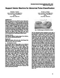
memory available. The programs of PWSVM, FPSSVM, and TSSVM are written in the MATLAB language. This computer runs Win7 with MATLAB 7.0.1. The source code of SSVM, “ssvm.m,” is obtained from the author’s website for the linear problem [24], and “lsvmk.m” for the nonlinear problem. In our experiments, all of the input data and the variables needed in programs are kept in the memory. For SSVM, TSSVM, FPSSVM, and PWSSVM, an optimality tolerance of 10−8 is used to determine when to terminate. Gaussian kernel is used in all our experiments. The first experiment is used to demonstrate the capability of PWSSVM in solving larger problems. The results in Table 1 are designed to compare the training correctness, the testing correctness, and the training time among the four smooth SVMs on a massively sized dataset. The datasets are created using Musicants NDC Data Generator [25] with different sizes. The test samples are 5% of the training samples. The experiment results show that PWSSVM has the highest training accuracy and testing accuracy. Furthermore, PWSSVM can be used to solve problems more quickly than the other three smooth SVMs when the number of the sample data is relative small. The second experiment is designed to demonstrate the effectiveness of PWSSVM through the “tried and true” checkerboard dataset [26]. One highly nonlinearly separable but simple example is the checkerboard dataset which has often been used to show the effectiveness of nonlinear kernel methods [17]. The checkerboard dataset is generated by uniformly discretizing the regions [0, 1] × [0, 1] to 2002 = 40000 points and labeling two classes “White” and “Black” spaced by 3 × 3 grid as Figure 2 shows.

6


Table 2: PWSSVM compared with SSVM, FPSSVM, and TSSVM on checkerboard dataset with difference sizes (𝐶 = 100). Training size

1000

2000

3000

5000

Train Test Algorithm correctness correctness (%) (%)

Time (s)

SSVM

99.60

98.28

4.61

FPSSVM TSSVM

99.60 99.62

98.28 98.28

4.35 4.23

PWSSVM

99.80

98.76

4.01

SSVM

98.84

98.54

11.97

FPSSVM TSSVM

99.22 99.22

98.59 98.59

9.63 9.35

PWSSVM

99.22

98.68

9.55

SSVM

98.47

98.88

25.21

FPSSVM TSSVM

98.64 98.68

98.88 98.90

21.58 17.21

PWSSVM

98.85

98.94

17.36

SSVM

99.34

99.51

47.09

FPSSVM TSSVM

99.48 99.52

99.51 99.51

39.29 38.76

PWSSVM

99.79

99.65

38.23

200

The rest results are presented in Table 2. The training set is randomly selected from the checkerboard with different sizes. The remaining samples are used as test samples. We compare the classification results of PWSSVM, TSSVM, FPSSVM, and SSVM with the same Gaussian kernel function. The results in Table 2 demonstrate that PWSSVM can solve massive problems quickly, followed by TSSVM, FPSVM, and SSVM in turn. The experimental results show that PWSSVM can obtain the highest train precision and test precision.

7. Conclusions A novel PWSSVM is proposed in this paper. It only needs to find the unique minima of the unconstrained differentiable convex quadratic function. The proposed method has many advantages over those available, such as good classification performance and less training time cost. The numerical results show that PWSSVM has excellent generalization ability.

Acknowledgments The authors would like to thank the anonymous reviewers for their valuable comments. This work was supported in part by the National Natural Science Foundation of China under Grants 61100165, 61100231, and 51205309 and the Natural Science Foundation of Shaanxi Province (2010JQ8004, 2012JQ8044).

References 150

100

50

0

0

50

100

150

200

Figure 2: The figure of the checkerboard dataset.

In the first trial of this experiment, the training set contains 1000 points randomly sampled from the checkerboard (for comparison, they are obtained from [17]) which contain 514 “white” samples and 486 “black” samples and the rest 39,000 points are in the testing set. Gaussian kernel function 𝐾(𝑥, 𝑦) = exp (−0.5 ||𝑥 − 𝑦||2 ) is used and 𝐶 = 100. Total time for the 1000-point training set using PWSSVM with a Gaussian kernel is 4.01 s. The train accuracy of PWSSVM is 99.80%. The test accuracy of PWSSVM is 98.76% on a 39,000point test set. TSSVM solves the same problem within 4.23 s, and the train accuracy and the test accuracy are 99.62% and 98.28%. FPSSVM and SSVM obtain the train accuracy of 99.60% within 4.35 s and 4.61 s, respectively. The test accuracy of them are 98.28%.

[1] V. N. Vapnik, The Nature of Statistical Learning Theory, Springer, New York, NY, USA, 1995. [2] V. N. Vapnik, Statistical Learning Theory, John Wiley & Sons, New York, NY, USA, 1998. [3] K. R. Mller, A. J. Smola, G. Rtsch, B. Schlkopf, J. Kohlmorgen, and V. Vapnik, “Using support vector machines for time series prediction,” in Advances in Kernel Methods: Support Vector Machine, B. Scholkopf, J. Burges, and A. Smola, Eds., MIT Press, Cambridge, Mass, USA, 1999. [4] T. Farooq, A. Guergachi, and S. Krishnan, “Knowledge-based Green’s Kernel for support vector regression,” Mathematical Problems in Engineering, vol. 2010, Article ID 378652, 16 pages, 2010. [5] J. Zheng and B. L. Lu Bao-Liang, “A support vector machine classifier with automatic confidence and its application to gender classification,” Neurocomputing, vol. 74, no. 11, pp. 1926– 1935, 2011. [6] J. Y. Zhu, B. Ren, H. X. Zhang, and Z. T. Deng, “Time series prediction via new support vector machines,” in Proceedings of the International Conference on Machine Learning and Cybernetics (ICMLC ’02), pp. 364–366, November 2002. [7] J. Ramana and D. Gupta, “LipocalinPred: a SVM-based method for prediction of lipocalins,” BMC Bioinformatics, vol. 10, p. 445, 2009. [8] T. Joachims, “Text categorization with support vector machines: learning with many relevant features,” in Proceedings of the 10th European Conference on Machine Learning (ECML ’98), pp. 137– 142, Springer, Heidelberg, Germany, 1998. [9] P. S. Jaume, M. I. Dar´ıo, and D. M. Fernando, “Support vector machines for continuous speech recognition,” in Proceedings of


[10]

[11]

[12]

[13]

[14]

[15]

[16]

[17]

[18]

[19]

[20]

[21]

[22] [23]

[24] [25] [26]

the 14th European Signal Processing Conference (EUSIPCO ’06), Florence, Italy, September 2006. V. Bevilacqua, P. Pannarale, M. Abbrescia, and C. Cava, “Comparison of data-merging methods with SVM attribute selection and classification in breast cancer gene expression,” BMC Bioinformatics, vol. 13, supplement 7, p. S9, 2012. E. J. Spinosa and A. C. Carvalho, “Support vector machines for novel class detection in bioinformatics,” Genetics and Molecular Research, vol. 4, no. 3, pp. 608–615, 2005. A. Nurettin and G. C¨uneyt, An Application of Support Vector Machine in Bioinformatics: Automated Recognition of Epileptiform Patterns in EEG Using SVM Classifier Designed by a Perturbation Method, vol. 3261 of Advances in Information Systems Lecture Notes in Computer Science, 2005. Y. F. Sun, X. D. Fan, and Y. D. Li, “Identifying splicing sites in eukaryotic RNA: support vector machine approach,” Computers in Biology and Medicine, vol. 33, no. 1, pp. 17–29, 2003. H. J. Lin and J. P. Yeh, “Optimal reduction of solutions for support vector machines,” Applied Mathematics and Computation, vol. 214, no. 2, pp. 329–335, 2009. A. Christmann and R. Hable, “Consistency of support vector machines using additive kernels for additive models,” Computational Statistics and Data Analysis, vol. 56, no. 4, pp. 854–873, 2012. Y. H. Shao and N. Y. Deng, “A coordinate descent margin based-twin support vector machine for classification,” Neural Networks, vol. 25, pp. 114–121, 2012. Y.-J. Lee and O. L. Mangasarian, “SSVM: a smooth support vector machine for classification,” Computational Optimization and Applications, vol. 20, no. 1, pp. 5–22, 2001. Y. B. Yuan, J. Yan, and C. X. Xu, “Polynomial smooth support vector machine (PSSVM),” Chinese Journal of Computers, vol. 28, no. 1, pp. 9–17, 2005. Y. B. Yuan and T. Z. Huang, A Polynomial Smooth Support Vector Machine for Classification, vol. 3584 of Lecture Note on Artificial Intelligence, 2005. J. Z. Xiong, J. L. Hu, H. Q. Yuan, T. M. Hu, and G. M. Li, “Research on a new class of functions for smoothing support vector machines,” Acta Electronica Sinica, vol. 35, no. 2, pp. 366– 370, 2007. Y. Yuan, W. Fan, and D. Pu, “Spline function smooth support vector machine for classification,” Journal of Industrial and Management Optimization, vol. 3, no. 3, pp. 529–542, 2007. D. P. Bertsekas, Nonlinear Programming, Athena Scientific, Belmont, Ma, USA, 2nd edition, 1999. C. Xu and J. Zhang, “A survey of Quasi-Newton equations and Quasi-Newton methods for optimization,” Annals of Operations Research, vol. 103, no. 1–4, pp. 213–234, 2001. D. R. Musicant and O. L. Managsarian, “LSVM: Lagrangian support vector machine,” 2000, http://www.cs.wisc.edu/dmi/svm/ . D. R. Musicant, “NDC: normally distributed clustered datasets,” 1998, http://www.cs.wisc.edu/∼musicant/data/ndc/ . T. K. Ho and E. M. Kleinberg, “Checkerboard dataset,” 1996, http://www.cs.wisc.edu/∼musicant/data/ndc/ .

7

Advances in

Operations Research Hindawi Publishing Corporation http://www.hindawi.com

Volume 2014

Advances in

Decision Sciences Hindawi Publishing Corporation http://www.hindawi.com

Volume 2014

Journal of

Applied Mathematics

Algebra

Hindawi Publishing Corporation http://www.hindawi.com


Volume 2014

Journal of

Probability and Statistics Volume 2014

The Scientific World Journal Hindawi Publishing Corporation http://www.hindawi.com


Volume 2014

International Journal of

Differential Equations Hindawi Publishing Corporation http://www.hindawi.com

Volume 2014

Volume 2014

Submit your manuscripts at http://www.hindawi.com International Journal of

Advances in

Combinatorics Hindawi Publishing Corporation http://www.hindawi.com

Mathematical Physics Hindawi Publishing Corporation http://www.hindawi.com

Volume 2014

Journal of

Complex Analysis Hindawi Publishing Corporation http://www.hindawi.com

Volume 2014

International Journal of Mathematics and Mathematical Sciences


Journal of

Mathematics Hindawi Publishing Corporation http://www.hindawi.com

Volume 2014


Volume 2014

Volume 2014


Volume 2014

Discrete Mathematics

Journal of

Volume 2014


Discrete Dynamics in Nature and Society

Journal of

Function Spaces Hindawi Publishing Corporation http://www.hindawi.com

Abstract and Applied Analysis

Volume 2014


Volume 2014


Volume 2014

International Journal of

Journal of

Stochastic Analysis

Optimization



Volume 2014

Volume 2014