In a nutshell, Osuna's theorem showed that the global SVM training problem can be broken down into a ... SVMs, the algorithm can be extremely slow on non-sparse data sets and on problems that have many support ..... Data Mining and.
Gary William Flake and Steve Lawrence. Efficient SVM Regression Training with SMO, accepted for publication, Machine Learning, 2001.
Efficient SVM Regression Training with SMO Gary William Flake
Steve Lawrence
flake�resear h.nj.ne . om
lawren e�resear h.nj.ne . om
NEC Research Institute 4 Independence Way Princeton, NJ 08540 Abstract — The sequential minimal optimization algorithm (SMO) has been shown to be an effective method for training support vector machines (SVMs) on classification tasks defined on sparse data sets. SMO differs from most SVM algorithms in that it does not require a quadratic programming solver. In this work, we generalize SMO so that it can handle regression problems. However, one problem with SMO is that its rate of convergence slows down dramatically when data is non-sparse and when there are many support vectors in the solution—as is the case in regression—because kernel function evaluations tend to dominate the runtime in this case. Moreover, caching kernel function outputs can easily degrade SMO’s performance even more because SMO tends to access kernel function outputs in an unstructured manner. We address these problem with several modifications that enable caching to be effectively used with SMO. For regression problems, our modifications improve converge time by over an order of magnitude. Keywords — support vector machines, sequential minimal optimization, regression, caching, quadratic programming, optimization
1
I NTRODUCTION
A support vector machine (SVM) is a type of model that is optimized so that prediction error and model complexity are simultaneously minimized [7]. Despite having many admirable qualities, research into the area of SVMs has been hindered by the fact that quadratic programming (QP) solvers provided the only known training algorithm for years. In 1997, a theorem [2] was proved that introduced a whole new family of SVM training procedures. In a nutshell, Osuna’s theorem showed that the global SVM training problem can be broken down into a sequence of smaller subproblems and that optimizing each subproblem minimizes the original QP problem. Even more recently, the sequential minimal optimization algorithm (SMO) was introduced [3, 5] as an extreme example of Osuna’s theorem in practice. Because SMO uses a subproblem of size two, each subproblem has an analytical solution. Thus, for the first time, SVMs could be optimized without a QP solver. While SMO has been shown to be effective on sparse data sets and especially fast for linear SVMs, the algorithm can be extremely slow on non-sparse data sets and on problems that have many support vectors. Regression problems are especially prone to these issues because the inputs are usually non-sparse real numbers (as opposed to binary inputs) with solutions that have many
support vectors. Because of these constraints, there have been no reports of SMO being successfully used on regression problems. In this work, we derive a generalization of SMO to handle regression problems and address the runtime issues of SMO by modifying the heuristics and underlying algorithm so that kernel outputs can be effectively cached. Conservative results indicate that for high-dimensional, non-sparse data (and especially regression problems), the convergence rate of SMO can be improved by an order of magnitude or more. This paper is divided into six additional sections. Section 2 contains a basic overview of SVMs and provides a minimal framework on which the later sections build. In Section 3, we generalize SMO to handle regression problems. This simplest implementation of SMO for regression can optimize SVMs on regression problems but with very poor convergence rates. In Section 4, we introduce several modifications to SMO that allow kernel function outputs to be efficiently cached. Section 5 contains numerical results that show that our modifications produce an order of magnitude improvement in convergence speed. Finally, Section 6 summarizes our work and addresses future research in this area.
2
I NTRODUCTION
TO
SVM S
(
)
(
)
Consider a set of data points, f x1 ; y1 ; � � � ; xN ; yN g, such that xi 2 R d is an input and yi is a target output. An SVM is a model that is calculated as a weighted sum of kernel function outputs. The kernel function can be an inner product, Gaussian basis function, polynomial, or any other function that obeys Mercer’s condition. Thus, the output of an SVM is either a linear function of the inputs, or a linear function of the kernel outputs. Because of the generality of SVMs, they can take forms that are identical to nonlinear regression, radial basis function networks, and multilayer perceptrons. The difference between SVMs and these other methods lies in the objective functions that they are optimized with respect to and the optimization procedures that one uses to minimize these objective functions. In the linear, noise-free case for classification, with yi 2 f ; g, the output of an SVM is x � w w0 , and the optimization task is defined as: written as f x; w
(
)=
+
minimize
11
1 jjwjj2 ; subject to y (x � w + w0 ) � 1 8i 2
(1)
i
Intuitively, this objective function expresses the notion that one should find the simplest model that explains the data. This basic SVM framework has been generalized to include slack variables for miss-classifications, nonlinear kernel functions, regression, as well as other extensions for other problem domains. It is beyond the scope of this paper to describe the derivation of all of these extensions to the basic SVM framework. Instead, we refer the reader to the excellent tutorials [1] and [6] for introductions to SVMs for classification and regression, respectively. We delve into the derivation of the specific objective functions only as far as necessary to set the framework from which we present our own work. In general, one can easily construct objective functions similar to Equation 1 that include slack variables for misclassification and nonlinear kernels. These objective functions can also be modified for the special case of performing regression, i.e., with yi 2 R instead of yi 2 f ; g. These objective functions will always have a component that should be minimizes and linear constraints that must be obeyed. To optimize the objective function, one converts it into the primal Lagrangian
11
2
form which contains the minimization terms minus the linear constraints multiplied by Lagrangian multipliers. The primal Lagrangian is converted into a dual Lagrangian where the only free parameters are the Lagrangian multipliers. In the dual form, the objective function is quadratic in the Lagrangian multipliers; thus, the obvious way to optimize the model is to express it as a quadratic programming problem with linear constraints. Our contribution in this paper uses a variant of Platt’s sequential minimal optimization method that is generalized for regression and is modified for further efficiencies. SMO solves the underlying QP problem by breaking it down into a sequence of smaller optimization subproblems with two unknowns. With only two unknowns, the parameters have an analytical solution, thus avoiding the use of a QP solver. Even though SMO does not use a QP solver, it still makes reference to the dual Lagrangian objective functions. Thus, we now define the output function of nonlinear SVMs for classification and regression, as well as the primal Lagrangian objective functions that they are optimized with respect to. In the case of classification, with yi � , the output of an SVM is defined as:
= 1
N X
f (x; �) =
(
i=1
)
yi �i K (xi ; x) + �0 ;
(2)
where K xa ; xb is the underlying kernel function. The primal objective function (which should be minimized) is:
1 X X y y � � K (x ; x ) X � ; L (�) = (3) 2 =1 =1 =1 P y � = 0: C is a usersubject to the box constraint 0 � � � C; 8 and the linear constraint =1 N
N
N
p
i j
i
i
j
i
j
j
i
i
i
N i
i
i
i
defined constant that represents a balance between the model complexity and the approximation error. Regression for SVMs minimize functionals of the form:
E (w) =
1 X jy N
N
f (xi ; w)j� + jjwjj2 ;
i
i=1
(4)
where j�j� is an �-insensitive error function defined as:
(
jxj� = j0xj �
if jxj < � otherwise
and the output of the SVM now takes the form of:
f (x; �� ; �) =
N X i=1
(��
�i )K (xi ; x) + �0 :
i
(5)
Intuitively, ��i and �i are “positive” and “negative” Lagrange multipliers (i.e., a single weight) that obey � ��i ; �i ; 8i and ��i �i ; 8i . The primal form of Equation 4 is written as
0
=0
Lp(�� ; �)
=
�
N X i=1
(�� + � )
N X N 1X
2
i
i
(��
i=1 j =1
i
3
N X i=1
yi (��i �i ) +
�i )(��j
�j )K (xi ; xj );
(6)
where one should minimize the objective function with respect to straints: N X i=1
(��
�i ) = 0;
i
�� and �, subject to the con-
0 � �� ; � � C; 8 : i
i
(7)
i
The parameter C is the same user-defined constant that represents a balance between the model complexity and the approximation error. In later sections, we will make extensive use of the two primal Lagrangians in Equations 3 and 6, and the SVM output functions in Equations 2 and 5.
3
SMO
AND
R EGRESSION
As mentioned earlier, SMO is a new algorithm for training SVMs. SMO repeatedly finds two Lagrange multipliers that can be optimized with respect to each other and analytically computes the optimal step for the two Lagrange multipliers. When no two Lagrange multipliers can be optimized, the original QP problem is solved. SMO actually consists of two parts: (1) a set of heuristics for efficiently choosing pairs of Lagrange multiplier to work on, and (2) the analytical solution to a QP problem of size two. It is beyond the scope of this paper to give a complete description of SMO’s heuristics. Instead, the reader should consult one of Platt’s papers [3, 5] for more information. Since SMO was originally designed (like SVMs) to only be applicable to classification problems, the analytical solution to the size two QP problem must be generalized in order for SMO to work on regression problems. The bulk of this section will be devoted to deriving this solution. 3.1
Step Size Derivation
=
= +
We begin by transforming Equations 5,6, and 7 by substituting �i ��i �i , and j�i j ��i �i . Thus, the new unknowns will obey the box constraint C � �i � C; 8i . We will also use the K xi ; xj and always assume that kij kji . The model output and objective shorthand kij function can now be written as:
= (
)
=
f (x; �)
=
Lp(�)
=
P
N X i=1
�
�i K (xi ; x) + �0 ;
N X i=1
j�ij
N X i=1
�i yi +
and
(8)
1 XX� � k 2 =1 =1 N
N
i j ij
i
;
(9)
j
=0
with the linear constraint N . Our goal is to express analytically the minimum of Equai=1 �i tion 9 as a function of two parameters. Let these two parameters have indices a and b so that �a and �b are the two unknowns. We can rewrite Equation 9 as
Lp(�a ; �b )
= � j� j + � j� j � y � y + 21 �2 k + 12 �2k + � � k + � v� + � v� + E ; a
a
b
b ab
a a
a a
a aa
b b
b b
b bb
(10)
where E is a term that is strictly constant with respect to �a and �b , and vi� is defined as
vi� =
X
j 6=a;b
��j kij = fi� ��a kai
4
��b kbi ��0
(11)
= (
)
f xi ; �� . Note that a superscript � is used above to explicitly indicate that values are with fi� computed with the old parameter values. This means that these portions of the expression will not be a function of the new parameters (which simplifies the derivation). P � , is true prior to any change to �a and �b , then If we assume that the constraint, N i=1 i in order for the constraint to be true after a step in parameter space, the sum of �a and �b must be held fixed. With this in mind, let s� �a �b ��a ��b . We can now rewrite Equation 10 as a function of a single Lagrange multiplier by substituting s� �b �a :
=0 = + = +
Lp (�b )
=
1 (s� � )2 k 2 � )v� + � v� + E :
= � js� � j + � j� j (s� � )y + 12 �2 k + (s� � )� k + (s� b
b
b bb
b
b
� b yb +
a
b ab
b
b
b b
a
aa
(12)
To solve Equation 12, we need to compute its partial derivative with respect to �b ; however, Equation 12 is not strictly differentiable because of the absolute value function. Nevertheless, if we take djxj=dx x , the resulting derivative is algebraically consistent:
= sgn( )
�Lp ��b
= �(sgn(� ) sgn(s� � )) + y y + (� s�)k + � k + (s� 2� )k b
b
aa
b
b bb
a
b
b
ab
va� + vb�
(13)
Now, setting Equation 13 to zero yields:
�b (kbb + kaa
2k ) = =
yb ya + �(sgn(�a ) sgn(�b )) + s� (kaa kab ) + va� vb� yb ya + fa� fb� + �(sgn(�a ) sgn(�b )) + ��a kaa ��a kab + ��b kaa ��b kab ��a kaa ��b kab ��0 + ��a kab + ��b kbb + ��0 yb ya + fa� fb� + �(sgn(�a ) sgn(�b )) + ��b (kbb + kaa 2kab )
ab
=
From Equation 14, we can write a recursive update rule for
�b = ��b +
=( +
1 [y
�
b
(14)
�b in terms of its old value:
ya + fa� fb� + �(sgn(�a )
2 )
sgn(� )); ℄
(15)
b
sgn( )
kbb kaa kab . While Equation 15 is recursive because of the two � functions, where � it still has a single solution that can be found quickly, as will be shown in the next subsection. 3.2
Finding Solutions
Figure 1 illustrates how the partial derivative (Equation 13) of the primal Lagrangian function with respect to �b behaves. If the kernel function of the SVM obeys Mercer’s condition (as all common kab � will always be true. If � is strictly ones do), then we are guaranteed that � kbb kaa positive, then Equation 13 will always be increasing. Moreover, if s� is not zero, then it will be piecewise linear with two discrete jumps, as illustrated in Figure 1. Putting these facts together means that we only have to consider five possible solutions for �a �b Equation 13. Three possible solutions correspond to using Equation 15 with
=
+
2
0
(sgn( ) sgn( ))
5
�E=��b
�b �a < 0 < �b
L
�
�
�b < 0 < � a
sgn( a ) = sgn( b )
0 (if s
�
> 0)
s� (if s�
s
�
< 0)
(if s
0 (if s�
�
> 0)
H
< 0)
Figure 1: The derivative as a function of �b : If the kernel function obeys Mercer’s condition, then the derivative (Equation 13) will always be strictly increasing.
set to -2, 0, and 2. The other two candidates correspond to setting �b to one of the transitions in or s� . Figure 1: �b We also need to consider how the linear and boxed constraints relate to one another. In particular, we need lower and upper bounds for �b that insure that both �a and �b are within the �C range. Using:
=0
L H
= max(s� C; C ) = min(C; s� + C )
(16) (17)
with L and H being the lower and upper bounds, respectively, guarantees that both parameters will obey the boxed constraints. 3.3
KKT Conditions
The step described in this section will only minimize the global objective function if one or both of the two parameters violates a KKT condition. The KKT conditions for regression are:
�i = 0 C < �i 6= 0 < C j�ij = C
() jyi fij < � () jyi fij = � () jyi fij > �:
(18)
These KKT conditions also yield a test for convergence. When no parameter violates any KKT condition, then the global minimum has been reached within machine precision.
6
3.4
Updating the Threshold
To update the SVM threshold, we calculate two candidate updates. The first update, if used along ya . The second forces fb yb . If neither with the new parameters, forces the SVM to have fa update for the other two parameters hits a constraint, then the two candidate updates for the threshold will be identical. Otherwise, we average the candidate updates.
=
�a0 �b0
= =
=
new old fa� ya + (�new �old �old a a )kaa + (�b b )kab + �0 new old �old �old fb� yb + (�new a a )kab + (�b b )kbb + �0
(19) (20)
These update rules are nearly identical to Platt’s original derivation. 3.5
Complete Update Rule
SMO can work on regression problems if the following steps are performed.
�
Pick two parameters, �a and �b , such that at least one parameter violates a KKT condition as defined in Equation 18.
�
Compute �raw b
(sgn( ) sgn( ))
– Try Equation 15 with �a �b equal to -2, 0, and 2. If the new value is a zero to Equation 13, then accept that as the new value. – If the above step failed, try �b equal to 0 or s� . Accept the value that has the property such that all positive (negative) perturbations yield a positive (negative) value for Equation 13.
� If �b > H , set �b = H . If �b < L, set �b = L. Otherwise, set �b = �b � Set �a = �a + �b �b . � Set �0 = 21 (�a0 + �b0) as specified in Equations 19 and 20. raw
new
new
old
old
raw
new
new
raw
.
new
new
The outer loop of SMO—that is, all of the non-numerical parts that make up the heuristics—can remain the same. As will be discussed in Section 5, further improvements can be made to SMO that improve the rate of convergence on regression problems by as much as an order of magnitude. 3.6
Simple Example
Figure 2 shows a plot of a scalar function which has been approximated with a nonlinear SVM. The SVM has a Gaussian kernel and was trained by the proposed algorithm with � set to 0.1. The true function is shown with a solid line, the SVM approximation is shown in a dashed line, and the resulting support vectors (i.e., the input points corresponding to non-zero Lagrange multipliers) are shown as points. As can be seen, the approximation is very reasonable given the choice of �.
7
1.5 True Function Approximation Support Vectors
1
0.5
0
-0.5
-1
-1.5 0
1
2
3
4
5
6
Figure 2: A simple SVM regression experiment: the true and approximated function are shown along with the calculated support vectors.
While further progress can be made: 1. If this is the first iteration, or if the previous iteration made no progress, then let the working set be all data points. 2. Otherwise, let the working set consist only of data points with non-bounded Lagrange multipliers. 3. For all data points in the working set, try to optimize the corresponding Lagrange multiplier. To find the second Lagrange multiplier: 3.1. Try the best one (found from looping over the non-bounded multipliers) according to Platt’s heuristic, or 3.2. Try all among the working set, or 3.3. Try to find one among the entire set of Lagrange multipliers. 4. If no progress was made and working set was all data points, then done. Table 1: Basic Pseudo-code for SMO
8
4
BUILDING
A
B ETTER SMO
As described in Section 2, SMO repeatedly finds two Lagrange multipliers that can be optimized with respect to each other and analytically computes the optimal step for the two Lagrange multipliers. Section 2 was concerned with the analytical portion of the algorithm. In this section, we concentrate on the remainder of SMO which consists of several heuristics that are used to pick pairs of Lagrange multipliers to optimize. While it is beyond the scope of this paper to give a complete description of SMO, Table 1 gives basic pseudo-code for the algorithm. For more information, consult one of Platt’s papers [3, 5]. Referring to Table 1, notice that the first Lagrange multiplier to work on is chosen at line 3; and its counterpart is chosen at line 3.1, 3.2, or 3.3. SMO attempts to concentrate its effort where it is most needed by maintaining a working set of non-bounded Lagrange multipliers. The idea is that Lagrange multipliers that are at bounds (either 0 or C for classification, or 0 or �C for regression) are mostly irrelevant to the optimization problem and will tend to keep their bounded values. At best, each optimization step will take time proportional to the number of Lagrange multipliers in the working set and, at worst, will take time proportional to the entire data set. However, the runtime is actually much slower than this analysis implies because each candidate for the second Lagrange multiplier requires three kernel functions to be evaluated. If the input dimensionality is large, then the kernel evaluations may be a significant factor in the time complexity. All told, we p � N � D ; where p is the can express the runtime of a single SMO step as O p � W � D probability that the second Lagrange multiplier is in the working set, W is the size of the working set, and D is the input dimensionality. The goal of this section is to reduce the runtime complexity for a single SMO step down to O p0 � W p0 � N � D , with p0 > p. Additionally, a method for reducing the total number of required SMO steps is also introduced, so we also reduce the cost of the outer most loop of SMO as well. Over the next five subsections, several improvements to SMO will be described. The most fundamental change is to cache the kernel function outputs. However, a naive caching policy actually slows down SMO since the original algorithm tends to randomly access kernel outputs with high frequency. Other changes are designed either to improve the probability that a cached kernel output can be used again or to exploit the fact that kernel outputs have been precomputed.
(
(
+ (1
4.1
)
+ (1
)
)
)
Caching Kernel Outputs
A cache is typically understood to be a small portion of memory that is faster than normal memory. In this work, we use cache to refer to a table of precomputed kernel outputs. The idea here is that frequently accessed kernel outputs should be stored and reused to avoid the cost recomputation. Our cache data structure contains an inverse index, I , with M entries such that Ii refers to the index (in the main data set) of the ith cached item. We maintain a two-dimensional M � M array to store the cached values. Thus, for any < i; j < M with a Ii and b Ij , we either have the precomputed value of kab stored in the cache or we have space allocated for that value and a flag set to indicate that the kernel output needs to be computed and saved. The cache can have any of the following operations applied to it:
1
�
=
=
query(a, b) — returns one of three values to indicate that kab is either (1) not in the cache, (2) allocated for the cache but not present, or (3) in the cache.
9
�
insert(a, b) — compute kab and force it into the cache, if it is not present already. The
� �
a
ess(a, b) — return kab by the fastest method available.
least recently used indices in I are replaced by a and b.
ti kle(a, b) — mark indices a and b as the most recently used elements.
We use a least recently used policy for updating the cache as would be expected but with the following exceptions:
� � �
For all i, kii is maintained in its own separate space since it is accessed so frequently. If SMO’s working set is all Lagrange multipliers (as determined in step 1 of Table 1), then all accesses to the cache are done without tickles and without inserts. If the working set is a proper subset and both requested indices are not in part of the working set, then the access is done with neither a tickle nor an insert.
As defined in this subsection, caching kernel outputs in SMO usually degrades the runtime because of the frequency of cache misses and the extra overhead incurred. This problem is even worse when the cache size is less than the number of support vectors in the solution. 4.2
Eliminating Thrashing
As shown in lines 3.1, 3.2, and 3.3 of Table 1, SMO uses a hierarchy of selection methods in order to find a second multiplier to optimize along with first. It first tries to find a very good one with a heuristic. If that fails, it settles for anything in the working set. But if that fails, SMO then starts searching through the entire training set. Line 3.3 causes problems in SMO for two reasons. First, it entails an extreme amount of work that results in only two multipliers changing. Second, if caching is used, line 3.3 could interfere with the update policies of the cache. To avoid these problems, we use a heuristic which entails a modification to SMO such that line 3.3 is executed only if the working set is the entire data set. We must execute it, in this case, to be sure that convergence is achieved. Platt [4] has proposed a modification with a similar goal in mind. In our example source code (which can be accessed via the URL given at the end of this paper) this heuristic corresponds to using the command-line option -lazy, which is short for “lazy loops”. 4.3
Optimal Steps
The next modification to SMO takes advantage of the fact that cached kernel outputs can be accessed in constant time. Line 3.1 of Table 1 searches over the entire working set and finds the multiplier that approximately yields the largest step size. However, if kernel outputs for two multipliers are cached, then computing the change to the objective function that results from optimizing the two multipliers takes constant time to calculate. Thus, by exploiting the cached kernel outputs, we can greedily take the step that yields the most improvement. Let �b be the first multiplier selected in line 3 of Table 1. For all a such that kab is cached, we can calculate new values for the two multipliers analytically and in constant time. Let the old values
10
for multipliers use � superscripts, as in ��a and ��a . Moreover, let fi and fi� be shorthand for the new and old values for the SVM output.1 The change to the classification objective function (Equation 3) that results from accepting the new multipliers is:
�L = p
�a ya (fa
1y � k 2 1y � k 2
a a aa
�0 ) ��a ya (fa�
1
1 y �� k 2
a a aa
��0 ) +
�0 ) ��b yb (fb� yb ��b kbb ��0 ) + �b yb (fb b b bb 2 kab (ya yb �a �b ya yb ��a ��b ) �a �b + ��a + ��b :
(21)
Equation 21 is derived by substituting � for � in Equation 3, and rewriting the equation so that all terms are trivially dependent or independent on �a and/or �b . Afterwards, the difference between two choices for the two multipliers can be calculated without any summations because the independent terms cancel. The change to the regression objective function (Equation 9) can be similarly calculated with:
�L = p
�a (fa ya �b (fb yb kab (��a ��b
1 � k � ) �� (f � y 1 �� k 0 2 2 1 � k �0) �� (f � y 1 ��k 2 2 � � ) + �(j� j j�� j + j� j j�� j): a aa
a
b bb
a
b
b
a
a
a
a aa
b
b
b
a
b bb
��0 ) + ��0 ) +
b
(22)
Thus, we modify SMO by replacing line 3.1 in Table 1 with code that looks for the best second multiplier via Equation 21 or 22 for all a such that kab is cached. In our example source code, this heuristic corresponds to using the command-line option -best, which is short for “best step”. 4.4
On Demand Incremental SVM Outputs
The next modification to SMO is a method to calculate SVM outputs more rapidly. Without loss of generality, assume we have an SVM that is used for classification and that the output of the SVM is determined from Equation 2 (but with � substituted for �). There are at least three different ways to calculate the SVM outputs after a single Lagrange multiplier, �j , has changed:
� � �
Use Equation 2, which is extremely slow. Change Equation 2 so that the summation is only over the nonzero Lagrange multipliers. Incrementally update the new value with fi
= f � + (� i
j
��j )yj kij .
Clearly, the last method is the fastest. SMO, in its original form, uses the third method to update the outputs whose multipliers are non-bounded (which are needed often) and the second method when an output is needed that has not been incrementally updated. We can improve on this method by only updating outputs when they are needed, and by computing which of the second or third method above is more efficient. To do this, we need two queues with Note that in this section, we refer to all Lagrange multipliers by � and not �. We do this to maintain consistency with earlier sections, even though this notation conflicts with Equations 3 and 6. 1
11
maximum sizes equal to the number of Lagrange multipliers and a third array to store a time stamp for when a particular output was last updated. Whenever a Lagrange multiplier changes value, we store the change to the multiplier and the change to �0 in the queues, overwriting the oldest value. When a particular output is required, if the number of time steps that have elapsed since the output was last updated is less than the number of nonzero Lagrange multipliers, we can calculate the output from its last known value and from the changed values in the queues. However, if there are fewer nonzero Lagrange multipliers, it is more efficient to update the output using the second method. Since the outputs are updated on demand, if the SVM outputs are accessed in a nonuniform manner, then this update method will exploit those statistical irregularities. In our example source code, this heuristic corresponds to using the command-line option - lever, which is short for “clever outputs”. 4.5
SMO with Decomposition
Using SMO with caching along with all of the proposed heuristics yields a significant runtime improvement as long as the cache size is at least as large as the number of support vectors in the solution. When the cache size is too small to fit all of the kernel outputs for each support vector pair, accesses to the cache will fail and runtime will be increased. This particular problem can be addressed by combining Osuna’s decomposition algorithm [2] with SMO. The basic idea is to iteratively build an M � M subproblem with < M < N , solve the subproblem, and then iterate with a new subproblem until the entire optimization problem is solved. However, instead of using a QP solver to solve the subproblem, we use SMO and chose M to be as large as the cache. The benefits of this combination are two-fold. First, much evidence indicates that decomposition can often be faster than using a QP solver. Since the combination of SMO and decomposition is functionally identical to standard decomposition with SMO as the QP solver, we should expect the same benefit. Second, using a subproblem that is the same size as the cache guarantees that all of the kernel outputs required will be available at every SMO iteration except for the first for each subproblem. However, we note that our implementation of decomposition is very naive in the way it constructs subproblems, since it essentially works on the first M randomly selected data points that violate a KKT condition. In our example source code, this heuristic corresponds to using the command-line option -ssz M , which is short for “subset size”.
2
5
E XPERIMENTAL R ESULTS
As a simple experiment, we model the Mackey-Glass delay-differential equation:
dx dt
= 1 +axx(10t (t � ) � )
bx(t)
= 17 = 0 2 = 0 1
with a regression SVM that uses Gaussian kernel functions. We use � ,a : , b : , and t = 1. The problem consists of 700 data points, 6 inputs with a delay value of 6, and forecasts are made 60 time steps into the future. Using � equal to 0.1 and Gaussian kernels with 0.5 variance, the solution has 40 support vectors. Hence, this problem is very simple.
�
12
Heuristics
none none none none
Subset 0 100 0 100
Cache 0 0 100 100
Time 7.893 5.836 5.754 3.615
Heuristics
all all all all
Subset 0 100 0 100
Cache 0 0 100 100
Time 7.063 5.905 1.266 0.724
Table 2: Experimental results: all results are averaged over ten trials. Entries where heuristics have the value of “all” indicate that “lazy loops” (from Section 4.2), “best step” (Section 4.3), and “clever outputs” (Section 4.4) are all used. The entries for Subset indicate the subset sized for decomposition (with “0” meaning no decomposition). All times are in CPU seconds on a 450 MHz Pentium II machine running Linux.
Table 2 shows the average runtime for this problem with several different experimental setups. As can be seen, the runtime difference between plain SMO and SMO with all of the proposed changes is an order of magnitude in size.
6
C ONCLUSIONS
This work has shown that SMO can be generalized to handle regression problems. The runtime of SMO can be greatly improved for large, dense, and high-dimensional data sets by adding caching along with other heuristics. The heuristics are designed to either improve the probability that cached kernel outputs will be used or exploit the fact that cached kernel outputs can be used in ways that are infeasible for non-cached kernel outputs. These changes are particularly beneficial for SMO used on regression problems because such problems typically have many support vectors in the solution. While the numerical result in Section 5 is very simple, the experiment is significant because of the problem’s simplicity. More specifically, had the problem had more data points, been of higher dimensionality, or had more support vectors in the solution, then the differences between plain SMO and modified SMO would have been even more pronounced. Preliminary results also indicate that these changes can greatly improve the performance of SMO on classification tasks that involve large, high-dimensional, and non-sparse data sets. Future work will concentrate on incremental methods that gradually increase numerical accuracy. Moreover, recursive decompositions may yield further improvements. Acknowledgements We thank Tommy Poggio, John Platt, Edgar Osuna, and Constantine Papageorgious for helpful discussions. Special thanks to Tommy Poggio and the Center for Biological and Computational Learning at MIT for hosting the first author during this research and to Eric Baum and the NEC Research Institute for funding a portion of the time to write up these results.
13
R EFERENCES [1] C. Burges. A tutorial on support vector machines for pattern recognition. Data Mining and Knowledge Discovery, 2(2):955–974, 1998. [2] E. Osuna, R. Freund, and F. Girosi. An improved training algorithm for support vector machines. In Proc. of IEEE NNSP’97, 1997. [3] J. Platt. Fast training of support vector machines using sequential minimal optimization. In B. Sch¨olkopf, C. Burges, and A. Smola, editors, Advances in Kernel Methods - Support Vector Learning. MIT Press, 1998. [4] J. Platt. Private communication, 1999. [5] J. Platt. Using sparseness and analytic QP to speed training of support vector machines. In M. S. Kearns, S. A. Solla, and D. A. Cohn, editors, Advances in Neural Information Processing Systems 11. MIT Press, 1999. [6] A. Smola and B. Sch¨olkopf. A tutorial on support vector regression. Technical Report NC2TR-1998-030, NeuroCOLT2, 1998. [7] V. Vapnik. The Nature of Statistical Learning Theory. Springer Verlag, New York, 1995.
14