SVM Tutorial: Classification, Regression, and Ranking Hwanjo Yu and Sungchul Kim
1 Introduction Support Vector Machines(SVMs) have been extensively researched in the data mining and machine learning communities for the last decade and actively applied to applications in various domains. SVMs are typically used for learning classification, regression, or ranking functions, for which they are called classifying SVM, support vector regression (SVR), or ranking SVM (or RankSVM) respectively. Two special properties of SVMs are that SVMs achieve (1) high generalization by maximizing the margin and (2) support an efficient learning of nonlinear functions by kernel trick. This chapter introduces these general concepts and techniques of SVMs for learning classification, regression, and ranking functions. In particular, we first present the SVMs for binary classification in Section 2, SVR in Section 3, ranking SVM in Section 4, and another recently developed method for learning ranking SVM called Ranking Vector Machine (RVM) in Section 5.
2 SVM Classification SVMs were initially developed for classification [5] and have been extended for regression [23] and preference (or rank) learning [14, 27]. The initial form of SVMs is a binary classifier where the output of learned function is either positive or negative. A multiclass classification can be implemented by combining multiple binary classifiers using pairwise coupling method [13, 15]. This section explains the moti-
Hwanjo Yu POSTECH, Pohang, South Korea, e-mail:
[email protected] Sungchul Kim POSTECH, Pohang, South Korea, e-mail:
[email protected]
1
2
Hwanjo Yu and Sungchul Kim
vation and formalization of SVM as a binary classifier, and the two key properties – margin maximization and kernel trick.
Fig. 1 Linear classifiers (hyperplane) in two-dimensional spaces
Binary SVMs are classifiers which discriminate data points of two categories. Each data object (or data point) is represented by a n-dimensional vector. Each of these data points belongs to only one of two classes. A linear classifier separates them with an hyperplane. For example, Fig. 1 shows two groups of data and separating hyperplanes that are lines in a two-dimensional space. There are many linear classifiers that correctly classify (or divide) the two groups of data such as L1, L2 and L3 in Fig. 1. In order to achieve maximum separation between the two classes, SVM picks the hyperplane which has the largest margin. The margin is the summation of the shortest distance from the separating hyperplane to the nearest data point of both categories. Such a hyperplane is likely to generalize better, meaning that the hyperplane correctly classify “unseen” or testing data points. SVMs does the mapping from input space to feature space to support nonlinear classification problems. The kernel trick is helpful for doing this by allowing the absence of the exact formulation of mapping function which could cause the issue of curse of dimensionality. This makes a linear classification in the new space (or the feature space) equivalent to nonlinear classification in the original space (or the input space). SVMs do these by mapping input vectors to a higher dimensional space (or feature space) where a maximal separating hyperplane is constructed.
SVM Tutorial: Classification, Regression, and Ranking
3
2.1 Hard-margin SVM Classification To understand how SVMs compute the hyperplane of maximal margin and support nonlinear classification, we first explain the hard-margin SVM where the training data is free of noise and can be correctly classified by a linear function. The data points D in Fig. 1 (or training set) can be expressed mathematically as follows. D = {(x1 , y1 ), (x2 , y2 ), ..., (xm , ym )}
(1)
where xi is a n-dimensional real vector, yi is either 1 or -1 denoting the class to which the point xi belongs. The SVM classification function F(x) takes the form F(x) = w · x − b.
(2)
w is the weight vector and b is the bias, which will be computed by SVM in the training process. First, to correctly classify the training set, F(·) (or w and b) must return positive numbers for positive data points and negative numbers otherwise, that is, for every point xi in D, w · xi − b > 0 if yi = 1, and w · xi − b < 0 if yi = −1
These conditions can be revised into: yi (w · xi − b) > 0, ∀(xi , yi ) ∈ D
(3)
If there exists such a linear function F that correctly classifies every point in D or satisfies Eq.(3), D is called linearly separable. Second, F (or the hyperplane) needs to maximize the margin. Margin is the distance from the hyperplane to the closest data points. An example of such hyperplane is illustrated in Fig. 2. To achieve this, Eq.(3) is revised into the following Eq.(4). yi (w · xi − b) ≥ 1, ∀(xi , yi ) ∈ D
(4)
Note that Eq.(4) includes equality sign, and the right side becomes 1 instead of 0. If D is linearly separable, or every point in D satisfies Eq.(3), then there exists such a F that satisfies Eq.(4). It is because, if there exist such w and b that satisfy Eq.(3), they can be always rescaled to satisfy Eq.(4) i )| The distance from the hyperplane to a vector xi is formulated as |F(x ||w|| . Thus, the margin becomes 1 (5) margin = ||w||
4
Hwanjo Yu and Sungchul Kim
Fig. 2 SVM classification function: the hyperplane maximizing the margin in a two-dimensional space
because when xi are the closest vectors, F(x) will return 1 according to Eq.(4). The closest vectors, that satisfy Eq.(4) with equality sign, are called support vectors. Maximizing the margin becomes minimizing ||w||. Thus, the training problem in SVM becomes a constrained optimization problem as follows. minimize: Q(w) = 21 ||w||2 subject to: yi (w · xi − b) ≥ 1, ∀(xi , yi ) ∈ D The factor of
1 2
(6) (7)
is used for mathematical convenience.
2.1.1 Solving the Constrained Optimization Problem The constrained optimization problem (6) and (7) is called primal problem. It is characterized as follows: • The objective function (6) is a convex function of w. • The constraints are linear in w. Accordingly, we may solve the constrained optimization problem using the method of Largrange multipliers [3]. First, we construct the Largrange function: m 1 J(w, b, α ) = w · w − ∑ αi {yi (w · xi − b) − 1} 2 i=1
(8)
SVM Tutorial: Classification, Regression, and Ranking
5
where the auxiliary nonnegative variables α are called Largrange multipliers. The solution to the constrained optimization problem is determined by the saddle point of the Lagrange function J(w, b, α ), which has to be minimized with respect to w and b; it also has to be maximized with respect to α . Thus, differentiating J(w, b, α ) with respect to w and b and setting the results equal to zero, we get the following two conditions of optimality:
Condition1 : Condition2 :
∂ J(w,b,α ) ∂w ∂ J(w,b,α ) ∂b
=0
(9)
=0
(10)
After rearrangement of terms, the Condition 1 yields m
w = ∑ αi yi , xi
(11)
i=1
and the Condition 2 yields m
∑ αi yi = 0
(12)
i=1
The solution vector w is defined in terms of an expansion that involves the m training examples. As noted earlier, the primal problem deals with a convex cost function and linear constraints. Given such a constrained optimization problem, it is possible to construct another problem called dual problem. The dual problem has the same optimal value as the primal problem, but with the Largrange multipliers providing the optimal solution. To postulate the dual problem for our primal problem, we first expand Eq.(8), term by term, as follows: m m m 1 J(w, b, α ) = w · w − ∑ αi yi w · xi − b ∑ αi yi + ∑ αi 2 i=1 i=1 i=1
(13)
The third term on the right-hand side of Eq.(13) is zero by virtue of the optimality condition of Eq.(12). Furthermore, from Eq.(11) we have m
m
w · w = ∑ αi yi w · x = ∑ i=1
m
∑ αi α j yi y j xi x j
(14)
i=1 j=1
Accordingly, setting the objective function J(w, b, α ) = Q(α ), we can reformulate Eq.(13) as m
Q(α ) = ∑ αi − i=1
where the αi are nonnegative. We now state the dual problem:
1 m m ∑ ∑ αi α j yi y j xi · x j 2 i=1 j=1
(15)
6
Hwanjo Yu and Sungchul Kim
maximize: Q(α ) = ∑ αi − 12 ∑ ∑ αi α j yi y j xi x j i
(16)
i j
subject to:
∑ αi yi = 0
(17)
α ≥0
(18)
i
Note that the dual problem is cast entirely in terms of the training data. Moreover, the function Q(α ) to be maximized depends only on the input patterns in the form of a set of dot product {xi · x j }m (i, j)=1 . Having determined the optimum Lagrange multipliers, denoted by αi∗ , we may compute the optimum weight vector w∗ using Eq.(11) and so write w∗ = ∑ αi∗ yi xi
(19)
i
Note that according to the property of Kuhn-Tucker conditions of optimization theory, The solution of the dual problem αi∗ must satisfy the following condition.
αi∗
αi∗ {yi (w∗ · xi − b) − 1} = 0 for i = 1, 2, ..., m
(20)
{yi (w∗ · xi − b) − 1}
or its corresponding constraint must be nonzero. and either This condition implies that only when xi is a support vector or yi (w∗ · xi − b) = 1, its corresponding coefficient αi will be nonzero (or nonnegative from Eq.(18)). In other words, the xi whose corresponding coefficients αi are zero will not affect the optimum weight vector w∗ due to Eq.(19). Thus, the optimum weight vector w∗ will only depend on the support vectors whose coefficients are nonnegative. Once we compute the nonnegative αi∗ and their corresponding suppor vectors, we can compute the bias b using a positive support vector xi from the following equation. b∗ = 1 − w∗ · xi
(21)
The classification of Eq.(2) now becomes as follows. F(x) = ∑ αi yi xi · x − b
(22)
i
2.2 Soft-margin SVM Classification The discussion so far has focused on linearly separable cases. However, the optimization problem (6) and (7) will not have a solution if D is not linearly separable. To deal with such cases, soft margin SVM allows mislabeled data points while still maximizing the margin. The method introduces slack variables, ξi , which measure
SVM Tutorial: Classification, Regression, and Ranking
7
the degree of misclassification. The following is the optimization problem for soft margin SVM. minimize: Q1 (w, b, ξi ) = 12 ||w||2 +C ∑ ξi
(23)
i
subject to:
yi (w · xi − b) ≥ 1 − ξi ,
ξi ≥ 0
∀(xi , yi ) ∈ D
(24) (25)
Due to the ξi in Eq.(24), data points are allowed to be misclassified, and the amount of misclassification will be minimized while maximizing the margin according to the objective function (23). C is a parameter that determines the tradeoff between the margin size and the amount of error in training. Similarily to the case of hard-margin SVM, this primal form can be transformed to the following dual form using the Lagrange multipliers. maximize: Q2 (α ) = ∑ αi − ∑ ∑ αi α j yi y j xi x j i
subject to:
(26)
i j
∑ αi yi = 0
(27)
C≥α ≥0
(28)
i
Note that neither the slack variables ξi nor their Lagrange multipliers appear in the dual problem. The dual problem for the case of nonseparable patterns is thus similar to that for the simple case of linearly separable patterns except for a minor but important difference. The objective function Q(α ) to be maximized is the same in both cases. The nonseparable case differs from the separable case in that the constraint αi ≥ 0 is replaced with the more stringent constraint C ≥ αi ≥ 0. Except for this modification, the constrained optimization for the nonseparable case and computations of the optimum values of the weight vector w and bias b proceed in the same way as in the linearly separable case. Just as the hard-margin SVM, α constitute a dual representation for the weight vector such that ms
w∗ = ∑ αi∗ yi xi
(29)
i=1
where ms is the number of support vectors whose corresponding coefficient αi > 0. The determination of the optimum values of the bias also follows a procedure similar to that described before. Once α and b are computed, the function Eq.(22) is used to classify new object. We can further disclose relationships among α , ξ , and C by the Kuhn-Tucker conditions which are defined by
αi {yi (w · xi − b) − 1 + ξi } = 0, i = 1, 2, ..., m and
(30)
8
Hwanjo Yu and Sungchul Kim
µi ξi = 0, i = 1, 2, ..., m
(31)
Eq.(30) is a rewrite of Eq.(20) except for the replacement of the unity term (1 − ξi ). As for Eq.(31), the µi are Lagrange multipliers that have been introduced to enforce the nonnegativity of the slack variables ξi for all i. At the saddle point the derivative of the Lagrange function for the primal problem with respect to the slack variable ξi is zero, the evaluation of which yields
αi + µi = C
(32)
By combining Eqs.(31) and (32), we see that
ξi = 0 if αi < C, and ξi ≥ 0 if αi = C
(33) (34)
We can graphically display the relationships among αi , ξi , and C in Fig. 3.
Fig. 3 Graphical relationships among αi , ξi , and C
Data points outside the margin will have α = 0 and ξ = 0 and those on the margin line will have C > α > 0 and still ξ = 0. Data points within the margin will have α = C. Among them, those correctly classified will have 1 > ξ > 0 and misclassified points will have ξ > 1.
2.3 Kernel Trick for Nonlinear Classification If the training data is not linearly separable, there is no straight hyperplane that can separate the classes. In order to learn a nonlinear function in that case, linear SVMs must be extended to nonlinear SVMs for the classification of nonlinearly separable
SVM Tutorial: Classification, Regression, and Ranking
9
data. The process of finding classification functions using nonlinear SVMs consists of two steps. First, the input vectors are transformed into high-dimensional feature vectors where the training data can be linearly separated. Then, SVMs are used to find the hyperplane of maximal margin in the new feature space. The separating hyperplane becomes a linear function in the transformed feature space but a nonlinear function in the original input space. Let x be a vector in the n-dimensional input space and ϕ (·) be a nonlinear mapping function from the input space to the high-dimensional feature space. The hyperplane representing the decision boundary in the feature space is defined as follows. w · ϕ (x) − b = 0
(35)
where w denotes a weight vector that can map the training data in the high dimensional feature space to the output space, and b is the bias. Using the ϕ (·) function, the weight becomes w = ∑ αi yi ϕ (xi ) (36) The decision function of Eq.(22) becomes m
F(x) = ∑ αi yi ϕ (xi ) · ϕ (x) − b
(37)
i
Furthermore, the dual problem of soft-margin SVM (Eq.(26)) can be rewritten using the mapping function on the data vectors as follows. Q(α ) = ∑ αi − i
1 ∑ αi α j yi y j ϕ (xi ) · ϕ (x j ) 2∑ i j
(38)
holding the same constraints. Note that the feature mapping functions in the optimization problem and also in the classifying function always appear as dot products, e.g., ϕ (xi ) · ϕ (x j ). ϕ (xi ) · ϕ (x j ) is the inner product between pairs of vectors in the transformed feature space. Computing the inner product in the transformed feature space seems to be quite complex and suffer from the curse of dimensionality problem. To avoid this problem, the kernel trick is used. The kernel trick replaces the inner product in the feature space with a kernel function K in the original input space as follows. K(u, v) = ϕ (u) · ϕ (v)
(39)
The Mercer’s theorem proves that a kernel function K is valid, if and only if, the following conditions are satisfied, for any function ψ (x). (Refer to [9] for the proof in detail.) Z
K(u, v)ψ (u)ψ (v)dxdy ≤ 0
where
Z
ψ (x)2 dx ≤ 0
(40)
10
Hwanjo Yu and Sungchul Kim
The Mercer’s theorem ensures that the kernel function can be always expressed as the inner product between pairs of input vectors in some high-dimensional space, thus the inner product can be calculated using the kernel function only with input vectors in the original space without transforming the input vectors into the highdimensional feature vectors. The dual problem is now defined using the kernel function as follows. maximize: Q2 (α ) = ∑ αi − ∑ ∑ αi α j yi y j K(xi , x j ) i
subject to:
(41)
i j
∑ αi yi = 0
(42)
C≥α ≥0
(43)
i
The classification function becomes: F(x) = ∑ αi yi K(xi , x) − b
(44)
i
Since K(·) is computed in the input space, no feature transformation will be actually done or no ϕ (·) will be computed, and thus the weight vector w = ∑ αi yi ϕ (x) will not be computed either in nonlinear SVMs. The followings are popularly used kernel functions. • Polynomial: K(a, b) = (a · b + 1)d • Radial Basis Function (RBF): K(a, b) = exp(−γ ||a − b||2 ) • Sigmoid: K(a, b) = tanh(κ a · b + c) Note that, the kernel function is a kind of similarity function between two vectors where the function output is maximized when the two vectors become equivalent. Because of this, SVM can learn a function from any shapes of data beyond vectors (such as trees or graphs) as long as we can compute a similarity function between any pairs of data objects. Further discussions on the properties of these kernel functions are out of the scope. We will instead give an example of using polynomial kernel for learning an XOR function in the following section.
2.3.1 Example: XOR problem To illustrate the procedure of training a nonlinear SVM function, assume we are given a training set of Table 1. Figure 4 plots the training points in the 2-D input space. There is no linear function that can separate the training points. To proceed, let K(x, xi ) = (1 + x · xi )2 (45) If we denote x = (x1 , x2 ) and xi = (xi1 , xi2 ), the kernel function is expressed in terms of monomials of various orders as follows.
SVM Tutorial: Classification, Regression, and Ranking
11
Input vector x Desired output y (-1, -1) -1 (-1, +1) +1 (+1, -1) +1 (+1, +1) -1 Table 1 XOR Problem
Fig. 4 XOR Problem
2 2 K(x, xi ) = 1 + x12 xi1 + 2x1 x2 xi1 xi2 + x22 xi2 + 2x1 xi1 + 2x2 xi2
(46)
The image of the input vector x induced in the feature space is therefore deduced to be √ √ √ ϕ (x) = (1, x12 , 2x1 x2 , x22 , 2x1 , 2x2 )
(47)
Based on this mapping function, the objective function for the dual form can be derived from Eq. (41) as follows. Q(α ) = α1 + α2 + α3 + α4 1 − (9α12 − 2α1 α2 − 2α1 α3 + 2α 1α4 2 +9α22 + 2α2 α3 − 2α2 α4 + 9α3 − 2α 3α4 + α42 )
(48)
Optimizing Q(α ) with respect to the Lagrange multipliers yields the following set of simultaneous equations:
12
Hwanjo Yu and Sungchul Kim
9α1 − α2 − α3 + α4 = 1 −α1 + 9α2 + α3 − α4 = 1
−α1 + α2 + 9α3 − α4 = 1 α1 − α2 − α3 + 9α4 = 1 Hence, the optimal values of the Lagrange multipliers are
α1 = α2 = α3 = α4 =
1 8
This result denotes that all four input vectors are support vectors and the optimum value of Q(α ) is Q(α ) =
1 4
and 1 1 ||w||2 = , 2 4
or
1 ||w|| = √ 2
From Eq.(36), we find that the optimum weight vector is 1 [−ϕ (x1 ) + ϕ (x2 ) + ϕ (x3 ) − ϕ (x4 )] 8 0 1 1 1 1 1 √ 1 √ 1 √ 1√ 0 1 2 − 2 − 2 2 − √ 1 + + − = 2 = − 8 1 √ 1 √ 1√ 1√ 0 − 2 − 2 2 2 0 √ √ √ √ 2 2 − 2 − 2 0
w=
(49)
The bias b is 0 because the first element of w is 0. The optimal hyperplane becomes 1 x12 √ −1 2x1 x2 =0 w · ϕ (x) = [0 0 √ 0 0 0] (50) x2 2 √2 2x1 √ 22 which reduces to −x1 x2 = 0
(51)
SVM Tutorial: Classification, Regression, and Ranking
13
−x1 x2 = 0 is the optimal hyperplane, the solution of the XOR problem. It makes the output y = 1 for both input points x1 = x2 = 1 and x1 = x2 = −1, and y = −1 for both input points x1 = 1, x2 = −1 or x1 = −1, x2 = 1. Figure. 5 represents the four points in the transformed feature space.
Fig. 5 The 4 data points of XOR problem in the transformed feature space
3 SVM Regression SVM Regression (SVR) is a method to estimate a function that maps from an input object to a real number based on training data. Similarily to the classifying SVM, SVR has the same properties of the margin maximization and kernel trick for nonlinear mapping. A training set for regression is represented as follows. D = {(x1 , y1 ), (x2 , y2 ), ..., (xm , ym )}
(52)
where xi is a n-dimensional vector, y is the real number for each xi . The SVR function F(xi ) makes a mapping from an input vector xi to the target yi and takes the form. F(x) =⇒ w · x − b
(53)
where w is the weight vector and b is the bias. The goal is to estimate the parameters (w and b) of the function that give the best fit of the data. An SVR function F(x)
14
Hwanjo Yu and Sungchul Kim
approximates all pairs (xi , yi ) while maintaining the differences between estimated values and real values under ε precision. That is, for every input vector x in D, yi − w · xi − b ≤ ε w · xi + b − yi ≤ ε
(54) (55)
1 ||w||
(56)
The margin is margin =
By minimizing ||w||2 to maximize the margin, the training in SVR becomes a constrained optimization problem as follows. minimize: L(w) = 12 ||w||2
(57)
subject to: yi − w · xi − b ≤ ε w · xi + b − yi ≤ ε
(58) (59)
The solution of this problem does not allow any errors. To allow some errors to deal with noise in the training data, The soft margin SVR uses slack variables ξ and ξˆ . Then, the optimization problem can be revised as follows. minimize: L(w, ξ ) = 21 ||w||2 +C ∑(ξi2 , ξˆi2 ), C > 0
(60)
i
subject to:
yi − w · xi − b ≤ ε + ξi , w · xi + b − yi ≤ ε + ξˆi ,
ξ , ξˆi ≥ 0
∀(xi , yi ) ∈ D ∀(xi , yi ) ∈ D
(61) (62) (63)
The constant C > 0 is the trade-off parameter between the margin size and the amount of errors. The slack variables ξ and ξˆ deal with infeasible constraints of the optimization problem by imposing the penalty to the excess deviations which are larger than ε . To solve the optimization problem Eq.(60), we can construct a Lagrange function from the objective function with Lagrange multipliers as follows:
SVM Tutorial: Classification, Regression, and Ranking
15
minimize: L = 21 ||w||2 +C ∑(ξi + ξˆi ) − ∑(ηi ξi + ηˆ i ξˆi ) i
(64)
i
− ∑ αi (ε + ηi − yi + w · xi + b) i
− ∑ αˆ i (ε + ηˆ i + yi − w · xi − b) i
η , ηˆ i ≥ 0 α , αˆ i ≥ 0
subject to:
(65) (66)
where ηi , ηˆ i , α , αˆ i are the Lagrange multipliers which satisfy positive constraints. The following is the process to find the saddle point by using the partial derivatives of L with respect to each lagrangian multipliers for minimizing the function L.
∂L = ∑(αi − αˆ i ) = 0 ∂b i
(67)
∂L = w − Σ (αi − αˆ i )xi = 0, w = ∑(αi − αˆ i )xi ∂w i
(68)
∂L = C − αˆ i − ηˆ i = 0, ηˆ i = C − αˆ i ∂ ξˆi
(69)
The optimization problem with inequality constraints can be changed to following dual optimization problem by substituting Eq. (67), (68) and (69) into (64). maximize: L(α ) = ∑ yi (αi − αˆi ) − ε ∑(αi + αˆi ) i
(70)
i
− 12 ∑ ∑(αi − αˆi )(αi − αˆi )xi x j
(71)
∑(αi − αˆi ) = 0
(72)
0 ≤ α , αˆ ≤ C
(73)
i j
subject to:
i
The dual variables η , ηˆ i are eliminated in revising Eq. (64) into Eq. (70). Eq. (68) and (68) can be rewritten as follows. w = ∑(αi − αˆ i )xi
(74)
i
ηi = C − αi ηˆ i = C − αˆ i
(75) (76)
where w is represented by a linear combination of the training vectors xi . Accordingly, the SVR function F(x) becomes the following function. F(x) =⇒ ∑(αi − αˆ i )xi x + b i
(77)
16
Hwanjo Yu and Sungchul Kim
Eq.(77) can map the training vectors to target real values with allowing some errors but it cannot handle the nonlinear SVR case. The same kernel trick can be applied by replacing the inner product of two vectors xi , x j with a kernel function K(xi , x j ). The transformed feature space is usually high dimensional, and the SVR function in this space becomes nonlinear in the original input space. Using the kernel function K, The inner product in the transformed feature space can be computed as fast as the inner product xi · x j in the original input space. The same kernel functions introduced in Section 2.3 can be applied here. Once replacing the original inner product with a kernel function K, the remaining process for solving the optimization problem is very similar to that for the linear SVR. The linear optimization function can be changed by using kernel function as follows. maximize: L(α ) = ∑ yi (αi − αˆi ) − ε ∑(αi + αˆi ) i
− 12
i
∑ ∑(αi − αˆi )(αi − αˆi )K(xi , x j )
(78)
i j
subject to:
∑(αi − αˆi ) = 0
(79)
αˆ i ≥ 0, αi ≥ 0 0 ≤ α , αˆ ≤ C
(80)
i
(81)
Finally, the SVR function F(x) becomes the following using the kernel function. F(x) =⇒ ∑(αˆ i − αi )K(xi , x) + b
(82)
i
4 SVM Ranking Ranking SVM, learning a ranking (or preference) function, has produced various applications in information retrieval [14, 16, 28]. The task of learning ranking functions is distinguished from that of learning classification functions as follows: 1. While a training set in classification is a set of data objects and their class labels, in ranking, a training set is an ordering of data. Let “A is preferred to B” be specified as “A ≻ B”. A training set for ranking SVM is denoted as R = {(x1 , yi ), ..., (xm , ym )} where yi is the ranking of xi , that is, yi < y j if xi ≻ x j . 2. Unlike a classification function, which outputs a distinct class for a data object, a ranking function outputs a score for each data object, from which a global ordering of data is constructed. That is, the target function F(xi ) outputs a score such that F(xi ) > F(x j ) for any xi ≻ x j . If not stated, R is assumed to be strict ordering, which means that for all pairs xi and x j in a set D, either xi ≻R x j or xi ≺R x j . However, it can be straightforwardly
SVM Tutorial: Classification, Regression, and Ranking
17
generalized to weak orderings. Let R∗ be the optimal ranking of data in which the data is ordered perfectly according to user’s preference. A ranking function F is typically evaluated by how closely its ordering RF approximates R∗ . Using the techniques of SVM, a global ranking function F can be learned from an ordering R. For now, assume F is a linear ranking function such that: ∀{(xi , x j ) : yi < y j ∈ R} : F(xi ) > F(x j ) ⇐⇒ w · xi > w · x j
(83)
A weight vector w is adjusted by a learning algorithm. We say an orderings R is linearly rankable if there exists a function F (represented by a weight vector w) that satisfies Eq.(83) for all {(xi , x j ) : yi < y j ∈ R}. The goal is to learn F which is concordant with the ordering R and also generalize well beyond R. That is to find the weight vector w such that w · xi > w · x j for most data pairs {(xi , x j ) : yi < y j ∈ R}. Though this problem is known to be NP-hard [10], The solution can be approximated using SVM techniques by introducing (non-negative) slack variables ξi j and minimizing the upper bound ∑ ξi j as follows [14]: minimize: L1 (w, ξi j ) = 12 w · w +C ∑ ξi j subject to: ∀{(xi , x j ) : yi < y j ∈ R} : w · xi ≥ w · x j + 1 − ξi j ∀(i, j) : ξi j ≥ 0
(84) (85) (86)
By the constraint (85) and by minimizing the upper bound ∑ ξi j in (84), the above optimization problem satisfies orderings on the training set R with minimal error. 1 ), it tries to maximize the By minimizing w · w or by maximizing the margin (= ||w|| generalization of the ranking function. We will explain how maximizing the margin corresponds to increasing the generalization of ranking in Section 4.1. C is the soft margin parameter that controls the trade-off between the margin size and training error. By rearranging the constraint (85) as w(xi − x j ) ≥ 1 − ξi j
(87)
The optimization problem becomes equivalent to that of classifying SVM on pairwise difference vectors (xi − x j ). Thus, we can extend an existing SVM implementation to solve the problem. Note that the support vectors are the data pairs (xsi , xsj ) such that constraint (87) is satisfied with the equality sign, i.e., w(xsi − xsj ) = 1 − ξi j . Unbounded support vectors are the ones on the margin (i.e., their slack variables ξi j = 0), and bounded support vectors are the ones within the margin (i.e., 1 > ξi j > 0) or misranked (i.e., ξi j > 1). As done in the classifying SVM, a function F in ranking SVM is also expressed only by the support vectors. Similarily to the classifying SVM, the primal problem of ranking SVM can be transformed to the following dual problem using the Lagrange multipliers.
18
Hwanjo Yu and Sungchul Kim
maximize: L2 (α ) = ∑ αi j − ∑ ∑ αi j αuv K(xi − x j , xu − xv )
(88)
i j uv
ij
C≥α ≥0
subject to:
(89)
Once transformed to the dual, the kernel trick can be applied to support nonlinear ranking function. K(·) is a kernel function. αi j is a coefficient for a pairwise difference vectors (xi − x j ). Note that the kernel function is computed for P2 (∼ m4 ) times where P is the number of data pairs and m is the number of data points in the training set, thus solving the ranking SVM takes O(m4 ) at least. Fast training algorithms for ranking SVM have been proposed [17] but they are limited to linear kernels. Once α is computed, w can be written in terms of the pairwise difference vectors and their coefficients such that: w = ∑ αi j (xi − x j )
(90)
ij
The ranking function F on a new vector z can be computed using the kernel function replacing the dot product as follows: F(z) = w · z = ∑ αi j (xi − x j ) · z = ∑ αi j K(xi − x j , z). ij
(91)
ij
4.1 Margin-Maximization in Ranking SVM
Fig. 6 Linear projection of four data points
We now explain the margin-maximization of the ranking SVM, to reason about how the ranking SVM generates a ranking function of high generalization. We first establish some essential properties of ranking SVM. For convenience of explana-
SVM Tutorial: Classification, Regression, and Ranking
19
tion, we assume a training set R is linearly rankable and thus we use hard-margin SVM, i.e., ξi j = 0 for all (i, j) in the objective (84) and the constraints (85). In our ranking formulation, from Eq.(83), the linear ranking function Fw projects data vectors onto a weight vector w. For instance, Fig. 6 illustrates linear projections of four vectors {x1 , x2 , x3 , x4 } onto two different weight vectors w1 and w2 respectively in a two-dimensional space. Both Fx1 and Fx2 make the same ordering R for the four vectors, that is, x1 >R x2 >R x3 >R x4 . The ranking difference of two vectors (xi , x j ) according to a ranking function Fw is denoted by the geometric distance of the two vectors projected onto w, that is, formulated as
w(xi −x j ) ||w|| .
Corollary 1. Suppose Fw is a ranking function computed by the hard-margin ranking SVM on an ordering R. Then, the support vectors of Fw represent the data pairs that are closest to each other when projected to w thus closest in ranking. Proof. The support vectors are the data pairs (xsi , xsj ) such that w(xsi − xsj ) = 1 in constraint (87), which is the smallest possible value for all data pairs ∀(xi , x j ) ∈ R. Thus, its ranking difference according to Fw (= them [24].
w(xsi −xsj ) ||w|| )
is also the smallest among
Corollary 2. The ranking function F, generated by the hard-margin ranking SVM, maximizes the minimal difference of any data pairs in ranking. Proof. By minimizing w · w, the ranking SVM maximizes the margin δ = w(xsi −xsj ) ||w||
1 ||w||
=
where (xsi , xsj ) are the support vectors, which denotes, from the proof of Corollary 1, the minimal difference of any data pairs in ranking. The soft margin SVM allows bounded support vectors whose ξi j > 0 as well as unbounded support vectors whose ξi j = 0, in order to deal with noise and allow small error for the R that is not completely linearly rankable. However, the objective function in (84) also minimizes the amount of the slacks and thus the amount of error, and the support vectors are the close data pairs in ranking. Thus, maximizing the margin generates the effect of maximizing the differences of close data pairs in ranking. From Corollary 1 and 2, we observe that ranking SVM improves the generalization performance by maximizing the minimal ranking difference. For example, consider the two linear ranking functions Fw1 and Fw2 in Fig. 6. Although the two weight vectors w1 and w2 make the same ordering, intuitively w1 generalizes better than w2 because the distance between the closest vectors on w1 (i.e., δ1 ) is larger than that on w2 (i.e., δ2 ). SVM computes the weight vector w that maximizes the differences of close data pairs in ranking. Ranking SVMs find a ranking function of high generalization in this way.
20
Hwanjo Yu and Sungchul Kim
5 Ranking Vector Machine: An Efficient Method for Learning the 1-norm Ranking SVM This section presents another rank learning method, Ranking Vector Machine (RVM), a revised 1-norm ranking SVM that is better for feature selectoin and more scalable to large data sets than the standard ranking SVM. We first develop a 1-norm ranking SVM, a ranking SVM that is based on 1-norm objective function. (The standard ranking SVM is based on 2-norm objective function.) The 1-norm ranking SVM learns a function with much less support vectors than the standard SVM. Thereby, its testing time is much faster than 2-norm SVMs and provides better feature selection properties. (The function of 1-norm SVM is likely to utilize a less number of features by using a less number of support vectors [11].) Feature selection is also important in ranking. Ranking functions are relevance or preference functions in document or data retrieval. Identifying key features increases the interpretability of the function. Feature selection for nonlinear kernel is especially challenging, and the fewer the number of support vectors are, the more efficiently feature selection can be done [12, 20, 6, 30, 8]. We next present RVM which revises the 1-norm ranking SVM for fast training. The RVM trains much faster than standard SVMs while not compromising the accuracy when the training set is relatively large. The key idea of RVM is to express the ranking function with “ranking vectors” instead of support vectors. Support vectors in ranking SVMs are pairwise difference vectors of the closest pairs as discussed in Section 4. Thus, the training requires investigating every data pair as potential candidates of support vectors, and the number of data pairs are quadratic to the size of training set. On the other hand, the ranking function of the RVM utilizes each training data object instead of data pairs. Thus, the number of variables for optimization is substantially reduced in the RVM.
5.1 1-norm Ranking SVM The goal of 1-norm ranking SVM is the same as that of the standard ranking SVM, that is, to learn F that satisfies Eq.(83) for most {(xi , x j ) : yi < y j ∈ R} and generalize well beyond the training set. In the 1-norm ranking SVM, we express Eq.(83) using the F of Eq.(91) as follows. P
P
ij
ij
F(xu ) > F(xv ) =⇒ ∑ αi j (xi − x j ) · xu > ∑ αi j (xi − x j ) · xv
(92)
P
=⇒ ∑ αi j (xi − x j ) · (xu − xv ) > 0
(93)
ij
Then, replacing the inner product with a kernel function, the 1-norm ranking SVM is formulated as:
SVM Tutorial: Classification, Regression, and Ranking
P
P
ij
ij
L(α , ξ ) = ∑ αi j +C ∑ ξi j
minimize :
21
(94)
P
s.t. : ∑ αi j K(xi − x j , xu − xv ) ≥ 1 − ξuv , ∀{(u, v) : yu < yv ∈ R}
(95)
ij
α ≥ 0, ξ ≥ 0
(96)
While the standard ranking SVM suppresses the weight w to improve the generalization performance, the 1-norm ranking suppresses α in the objective function. Since the weight is expressed by the sum of the coefficient times pairwise ranking difference vectors, suppressing the coefficient α corresponds to suppressing the weight w in the standard SVM. (Mangasarian proves it in [18].) C is a user parameter controlling the tradeoff between the margin size and the amount of error, ξ , and K is the kernel function. P is the number of pairwise difference vectors (∼ m2 ). The training of the 1-norm ranking SVM becomes a linear programming (LP) problem thus solvable by LP algorithms such as the Simplex and Interior Point method [18, 11, 19]. Just as the standard ranking SVM, K needs to be computed P2 (∼ m4 ) times, and there are P number of constraints (95) and α to compute. Once α is computed, F is computed using the same ranking function as the standard ranking SVM, i.e., Eq.(91). The accuracies of 1-norm ranking SVM and standard ranking SVM are comparable, and both methods need to compute the kernel function O(m4 ) times. In practice, the training of the standard SVM is more efficient because fast decomposition algorithms have been developed such as sequential minimal optimization (SMO) [21] while the 1-norm ranking SVM uses common LP solvers. It is shown that 1-norm SVMs use much less support vectors that standard 2norm SVMs, that is, the number of positive coefficients (i.e., α > 0) after training is much less in the 1-norm SVMs than in the standard 2-norm SVMs [19, 11]. It is because, unlike the standard 2-norm SVM, the support vectors in the 1-norm SVM are not bounded to those close to the boundary in classification or the minimal ranking difference vectors in ranking. Thus, the testing involves much less kernel evaluations, and it is more robust when the training set contains noisy features [31].
5.2 Ranking Vector Machine Although the 1-norm ranking SVM has merits over the standard ranking SVM in terms of the testing efficiency and feature selection, its training complexity is very high w.r.t. the number of data points. In this section, we present Ranking Vector Machine (RVM), which revises the 1-norm ranking SVM to reduce the training time substantially. The RVM significantly reduces the number of variables in the optimization problem while not compromizing the accuracy. The key idea of RVM is to express the ranking function with “ranking vectors” instead of support vectors.
22
Hwanjo Yu and Sungchul Kim
The support vectors in ranking SVMs are chosen from pairwise difference vectors, and the number of pairwise difference vectors are quadratic to the size of training set. On the other hand, the ranking vectors are chosen from the training vectors, thus the number of variables to optimize is substantially reduced. To theoretically justify this approach, we first present the Representer Theorem. Theorem 1 (Representer Theorem [22]). Denote by Ω : [0, ∞) → R a strictly monotonic increasing function, by X a set, and by c : (X × R 2 )m → R ∪ {∞} an arbitrary loss function. Then each minimizer F ∈ H of the regularized risk c((x1 , y1 , F(x1 )), ..., (xm , ym , F(xm ))) + Ω (||F||H )
(97)
admits a representation of the form m
F(x) = ∑ αi K(xi , x)
(98)
i=1
The proof of the theorem is presented in [22]. Note that, in the theorem, the loss function c is arbitrary allowing coupling between data points (xi , yi ), and the regularizer Ω has to be monotonic. Given such a loss function and regularizer, the representer theorem states that although we might be trying to solve the optimization problem in an infinitedimensional space H , containing linear combinations of kernels centered on arbitrary points of X , the solution lies in the span of m particular kernels – those centered on the training points [22]. Based on the theorem, we define our ranking function F as Eq.(98), which is based on the training points rather than arbitrary points (or pairwise difference vectors). Function (98) is similar to function (91) except that, unlike the latter using pairwise difference vectors (xi − x j ) and their coeifficients (αi j ), the former utilizes the training vectors (xi ) and their coefficients (αi ). With this function, Eq.(92) becomes the following. m
m
i m
i
F(xu ) > F(xv ) =⇒ ∑ αi K(xi , xu ) > ∑ αi K(xi , xv ) =⇒ ∑ αi (K(xi , xu ) − K(xi , xv )) > 0.
(99) (100)
i
Thus, we set our loss function c as follows. c=
∑
∀{(u,v):yu