International Journal of Industrial Engineering, 22(4), 468-481, 2015
EFFICIENT SYNTACTIC PROCESS DIFFERENCE DETECTION AND ITS APPLICATION TO PROCESS SIMILARITY SEARCH Keqiang Liu1,2, Zhiqiang Yan2,*, Yuquan Wang3, Lijie Wen3, and Jianmin Wang3 1
School of Computer Science and Technology Beijing Institute of Technology Beijing, China 2
Information School Capital University of Economics and Business Beijing, China * Corresponding author’s e-mail:
[email protected] 3
School of Software Tsinghua University Beijing, China Nowadays, business process management plays an important role in the management of organizations. More and more organizations describe their operations as business processes. It is common for organizations to have collections of thousands of business process models. The same process is usually modeled differently due to the different rules or habits of different organizations and departments. Even in the subsidiaries of the same organization, process models vary from each other, because these process models are redesigned from time to time to continuously enhance the efficiency of management and operations. Therefore, techniques are required to analyze differences between similar process models. Current techniques can detect operations required to modify one process model to the other. However, these operations are based on activities and the syntactic meanings are limited. In this paper, we define differences based on workflow patterns and propose a technique to detect these differences efficiently. Besides that we propose a metric that can compute process similarity based on detected syntactic differences. To the best of our knowledge, this is the first technique that returns a list of syntactic differences while computing a similarity score between two process models. The experiment shows that these differences indeed exist in real-life process models and are useful to analyze differences between business process models; the experiment also shows that the metric for process similarity based on detected differences works well in terms of the quality of similarity search and the average precision score is 0.8. Keywords: business process model, syntactic difference, process similarity, process feature (Received on November 7, 2014; Accepted on June 18, 2015) 1. INTRODUCTION Recently, organizations tend to enhance their management efficiency with the technology of business process management (BPM). More and more business processes are described as process models to facilitate the implementation of BPM. Therefore, it is common to see thousands of process models in an organization or even in a department. For example, the information department of China Mobile Communication Corporation (CMCC) maintains more than 8,000 processes in its BPM systems (Gao et al. 2013). To manage such a large number of process models efficiently and automatically, business process model repositories are required (La Rosa et al. 2011, Yan et al. 2010, 2012). These repositories provide techniques include detecting differences between process models (Dijkman et al. 2008), process similarity search (Yan et al. 2012) and process querying (Yan et al. 2012). This paper focuses on detecting (syntactic) differences between business process models. Difference detection can, for example in case of merger between BPM systems of two or more organizations, be applied to detecting differences between two process models describing the same operation in different organizations. For example, originally each of the 34 subsidiaries of CMCC built its own BPM systems to maintain its business processes, but later the headquarters decided to build a unified one to maintain business process models of all subsidiaries (Gao et al. 2013). Since these subsidiaries have almost the same business processes, these process models are similar with some variations. For each business process, the headquarters also would like to have one model that works for different scenarios of all subsidiaries instead of to maintain different models for different scenarios. Therefore, it is required to have a technique that can detect the differences ISSN 1943-670X
© INTERNATIONAL JOURNAL OF INDUSTRIAL ENGINEERING
Liu et al.
Process Difference Detection
between these similar process models. A further application of difference detection is process model editing. In the case of modifying one process model to another, we can edit one fragment related to a difference instead of operating one activity at a time. Figure 1 shows two similar business process models describing a “receiving goods” process. Both models are in the BPMN notation. Given two similar process models, the technique in this paper identifies the difference patterns between these models. For example, in Figure 1, activity “Inbound Delivery Entered” in Model 1 and activity “Inbound Delivery Created” in Model 2 are interchanged activities; F1.1 of Model 1 has an additional dependency, “Invoice received”, compared with F2.1 of Model 2; F1.2 of Model 1 has different conditions compared with F2.2 of Model 2 because of different gateways. The technique in this paper detects these differences between process models efficiently. There currently exist techniques (Kuster et al. 2008; Li et al. 2008) that can analyze syntactic differences between process models. However, the focus of these techniques is computing the operations of modifying one process model to another. In this paper, the technique focuses on differences based on common workflow patterns, therefore provides more syntactic meanings about differences between process models. The experiment shows that the differences presented in this paper exist in real-life process models. Therefore, they are valuable for analyzing business process models. The contribution of this paper is as following: • syntactic differences are summarized and flexible feature matching is proposed for difference detection; • an algorithm is presented to show the steps to detect differences using flexible feature matching. • a metric is proposed to compute similarity between process models based on detected differences.
F1.1 Goods Received AND
Model 1
Inbound Delivery Entered
F1.2 Goods Recepit Processing with Reference
XOR Goods Recepit Processing
Invoice Received F2.1 Goods Received
Model 2
AND Inbound Delivery Created Inward Material Movement to be Posted
Goods Recepit Posted
F2.2
Goods Recepit Processing with Reference AND
F2.3
Goods Recepit Posted
Goods Recepit Processing
Figure 1. Two business process models about receiving goods in BPMN This paper extends our previous work (Liu et al. 2014). The major difference between this paper and (Liu et al. 2014) is the similarity metric, i.e., the third contribution listed above. Also an experiment is run to evaluate the similarity metric. The rest of the paper is organized as follows. Section 2 presents preliminaries of the technique of this paper. Section 3 and 4 presents exact and flexible feature matching respectively. Section 5 presents different types of syntactic differences and shows how to detect these differences using flexible feature matching. Section 6 presents the steps of detecting differences between two business process models. Section 7 presents how to compute similarity between process models based on detected differences. Section 8 presents the experiment. Section 9 presents related work and Section 10 concludes the paper. 469
Liu et al.
Process Difference Detection
2. PRELIMINARIES The technique in this paper is presented in the context of business process. A business process graph is a graph representation of a business process model (Dijkman et al. 2009), as described in Definition 1. As such, it focuses purely on the structure of that model, while abstracting from other aspects, e.g., different types of process modeling notations (BPMN, EPC, Petri net, etc.). Our detection of differences is based on the labels and structure of a business process model; therefore, abstracting from these aspects is acceptable. Due to the abstraction, types of nodes are also ignored, but we can still know which node is a gateway node from its label, e.g., xor, and from the size of its pre-set or post-set, e.g., a node has multiple nodes in its post-set. For example, Figure 2 shows the business process graphs for the models from Figure 1. Definition 1 (Business Process Graph, Pre-set, Post-set). Let L be a set of labels. A business process graph is a tuple (N, E, λ), in which: • N = A∪GW is the set of nodes, which consists of a set of activity nodes A and a set of gateway nodes GW; • E ⊆ N × N is the set of edges; and • λ: N → L is a function that maps nodes to labels. Let G = (N, E, λ) be a business process graph and n ∈ N be a node: •n = {m | (m, n) ∈ E} is the pre-set of n, while n• = {m | (n, m) ∈ E} is the post-set of n.
F1.1
F1.2
a
AND
Graph 1
d
b XOR
c
f
e
F2.1 a
F2.2 AND
Graph 2
d
b’
AND
F2.3 g
e
Figure 2. Business process graphs
470
f
Liu et al.
Process Difference Detection
a
a AND
AND b
b XOR c
c
f
XOR
f
e
e
Complex Join 2
Complex Join 1
Figure 3. Complex Join Features We consider features based on the most common workflow patterns: sequence, split, join, and loop. Definition 2 provides a formal description of these features (Yan et al. 2012). Definition 2 (Feature). Let g = (N, E, λ) be a process graph. A feature f of G is a subgraph of g. The size of a feature is the number of edges it contains. A feature is a: • sequence feature of size s−1 consisting of nodes { n1 , n2 , n3 ,. . . , ns }, if Ef is the minimal set containing ( n1 , n2 ), ( n2 , n3 ), . . . , ( ns-1 , ns ), for s ≥ 2; • split feature of size s + 1 consisting of a split node n, a node m and a set of nodes { n1 , n2, n3 , . . . , ns }, if and only if Ef is the minimal set containing ( m , n ), ( n , n1 ), ( n , n2 ), . . . , ( n , ns ), for s ≥ 2; • join feature of size s + 1 consisting of a join node n, a node m and a set of nodes { n1,, n2, n3 , . . . , ns }, if and only if Ef is the minimal set containing ( n1 , n ), ( n2 , n ), . . . , ( ns , n ), ( n , m ), for s ≥ 2; • loop feature of size s consisting of nodes { n1 , n2 , . . . , ns }, if Ef is the minimal set containing ( n1 , n2 ), . . . , ( ns-1 , ns ), ( ns , n1 ) for s ≥ 1. Some feature can further be decomposed into features, e.g., feature F1.1 contains three subgraphs that are join features with two branches. However, we do not need to reconsider these subgraphs when we detect differences. Therefore, only local maximal features, as defined in Definition 3 need to be gotten from process graphs. For example, in Figure 2 features of Graph 1 and Graph 2 are circled in dash-dotted boxes. There are one local maximal sequence feature (F2.3) and four local maximal join features. Definition 3 (Local Maximal Feature). Let g = (A∪GW, E, λ) be a process graph. A subgraph of g, f = ((A1∪GW 1 ), E1 , λ) is a feature. Feature f is a local maximal feature if and only if there exists no subgraph f’ in g, such that f’ is a feature of g and f is a subgraph of f’. We also notice that multiple split/join gateways may connect to each other as shown in Figure 3. Differences may occur between fragments like that. For example, the two fragments in Figure 3 have different conditions because they consist of the same set of activities but have different behaviors. Therefore, we define complex split and join features to be able to identify differences in complex structures like that. Definition 4 (Complex Join/Split Feature). Let g = (A∪GW, E, λ) be a process graph. A subgraph of g, f = ((A1∪GW1 ), E1 , λ) is a complex join feature if and only if: • GW1
GW (|GW1 | > 1),
gw ∈ GW1 , | gw•| = 1 ∧ |• gw| ≥ 2 ∧ ( gw1 ∈ GW1 ∧ gw1 ǂ gw , such that
gw1 ∈ gw• ∨gw1 ∈ •gw); • A1
A (|A1 | > 2),
a ∈ A1 , gw ∈ GW1 , such that a ∈ gw• ∨a ∈ •gw;
• E1 = E ∩ ((A1 ∪ GW1 ) × (A1 ∪ GW1 )). Complex split feature can be defined analogously. 471
Liu et al.
Process Difference Detection
3. EXACT FEATURE MATCHING We analyze nodes based on their label similarities. Label similarity can be measured in a number of different ways (van Dongen et al. 2008). For illustration purposes we will use a syntactic similarity metric, which is based on string edit-distance, in this paper. However, more advanced metrics can be used that take synonyms and stemming (van Dongen 2008) and, if possible, domain ontologies into account (Ehrig et al. 2007). The label similarity and label matching are defined in the former work (Dijkman et al. 2009). Definition 5 (Label Distance, Label Similarity, Node Matching). Let G = (N, E, λ) be a business process graph and n, m ∈ N be two nodes and let |x| represent the number of characters in a label x. The string edit distance of the labels λ(n) and λ(m) of the nodes, denoted ed(λ(n), λ(m)) is the minimal number of atomic string operations needed to transform λ(n) into λ(m) or vice versa. The atomic string operations are: inserting a character, deleting a character or substituting a character for another. The label distance of λ(n) and λ(m), denoted ldis(n, m) is: ldis(n,m)=
!"(! ! ,! ! ) !"# (|! ! |,|! ! |)
(1)
The label feature similarity of λ(n) and λ(m), denoted lsim(n, m) is: lsim(n, m) = 1.0 - ldis(n, m). Let lcutoff be a cutoff value for node matching, which can be assigned as desired. Given two nodes n and m, they are matched, denoted as match(n1 , n2), if and only if their label similarity is no less than lcutoff, i.e., lsim (n, m) >= lcutoff. ! For example, the similarity of label “Inbound Delivery Entered” and label “Inbound Delivery Created” is 1.0- = !! 0.79. They are matched given a cutoff 0.75. We consider two structural features to be matched, if their components (nodes and edges) are matched (Yan et al. 2012). Definition 6 (Exact Feature Matching). Given two features f1 = (N1, E1, λ1) and f2 = (N2, E2, λ2), they are matched, denoted as match(f1, f2) if and only if, there exists a bijection M: N1 → N2, such that • |N1 | = |N2 |; •
n ∈ N1 , match(n, M (n));
• |E1 | = |E2 |; •
(n1 , n2 ) ∈ E1 , (M (n1 ), M (n2 )) ∈ E2.
For example, two sequence features of size s with lists of nodes Ln = [n1 , n2 , n3 , . . . , ns ] and Lm = [m1 , m2 , m3 , . . . , ms ] are matched if and only if for each 1 ≤ i ≤ s: the node features of ni and mi are matched. 4. FLEXIBLE FEATURE MATCHING In the previous section, we explain features and their exact matching. We know that the rules for exact feature matching are strict in their structure, i.e., two features of different types or sizes are never matched with each other. This can help identify the common features in two process graphs but makes it difficult to identify the differences. Therefore, in this section, we define two types of flexible feature matching and in the next section we show how to solve this issue with flexible feature matching. The first type is called the subgraph-flexible feature matching. In this type, two features are not matched, but there exists a subgraph of one feature is matched with a subgraph of the other. For example, in Figure 2 F1.1 of Graph 1 and F2.1 of Graph 2 are subgraph-flexible feature matching. Definition 7 (Subgraph-flexible Feature Matching). Given two features f1 = (A1∪GW1, E1 , λ) and f2 = (A2∪GW2, E2 , λ), they are not exact feature matching. They are subgraph-flexible matched, denoted as FmatchSub (f1 , f2 ) if and only if, there exists a subgraph f 1’ = (A1’ ,∪GW1’, E 1’, λ) of f1 and a subgraph f 2’ = (A2’ ∪ GW 2’, E 2’, λ) of f2 , such that • |A1’ | = |A2’ | > 0; • match(f 1’, f 2’); • ( n1 ∈ ( A1 - A1’) , ∄n2∈ ( A2 – A2’) , match (n1 , n2)) ∨( n2 ∈ ( A2 – A2’) , ∄n1∈ ( A1 – A1’) , match (n1 , n2)). 472
Liu et al.
Process Difference Detection
The second type is the gateway-flexible feature matching. In this type, there exists a one-to-one mapping between activities of two features and each pair of mapped activities is matched. For example, in Figure 2, F1.2 of Graph 1 and F2.2 of Graph 2 are gateway-flexible feature matching, two complex features in Figure 3 are also gateway-flexible feature matching. Definition 8 (Gateway-flexible Feature Matching). Given two features f1 = (A1∪GW1, E1, λ) and f2 = (A2∪ GW2 , E2 , λ), they are neither exact feature matching nor subgraph-flexible feature matching. Then f1 and f2 are gateway-flexible matching, denoted as FmatchGate (f1, f2), if and only if 1. there exists a bijection M: A1→ A2, such that • |A1 | = |A2 |; • ∀a ∈ A1, match (a, M(a)). 2.
when GW1 and GW2 are not empty sets at the same time, there exists no bijection M’: GW1→ GW2 , ∀gw ∈ GW1 •∀a ∈ A1, such that (∀(a,gw)∈E1, (M (a), M’(gw))∈E2) ∧ (∀(gw,a)∈E1, (M’ (gw), M(a))∈E2); •∀gw’∈ GW1, such that (∀(gw’,gw)∈E1, (M’ (gw’), M’(gw))∈E2) ∧ (∀(gw,gw’)∈E1, (M’ (gw), M’(gw’))∈E2).
5. DETECTING DIFFERENCES WITH FLEXIBLE FEATURE MATCHING This section presents different types of syntactic differences between process models considered in this paper and how to detect these differences using flexible feature matching. Firstly, we present differences on nodes, which are basis of other differences. Given two business process graphs, provided that an activity does not have identical label with activities in the other graph, the activity is a skipped activity if no activities are matched with it; otherwise it is an interchanged activity. For example, in Figure 2, activity c (“Invoice received”) is a skipped activity; activity b (“Inbound Delivery Entered” ) and activity b’ “Inbound Delivery Created” are interchanged activities. Definition 9 (Skipped Activity (SA), Interchanged Activities (IA)). Let g1 = (N1, E1, λ) and g2 = (N2, E2, λ) be two business process graphs. Given a node n1 ∈ N1, n1 is a skipped activity, if and only if there exists no node n2 ∈ N2 matches with n1, i.e., ∄n2 ∈ N2, match (n1, n2); n1 and n2 are interchanged activities, if and only if there exists a node n2 ∈ N2 labeled differently matches with n1, i.e., ∄n2 ∈ N2, match (n1, n2) ∧ λ(n1) ǂ λ(n2). Then, we present differences on features, including additional branches, different branches, different order, different routing, and loop2once-off. Figure 4 shows an example for each type of difference considered in this paper. In the following content, each difference and how to detect it with features are explained. 5.1. Differences Related to Subgraph-flexible Feature Matching This sub-section describes two types of differences that can be detected using subgraph-flexible feature matching. Difference additional branches indicates that one join/split feature has additional branch(es) than the other join/split or sequence feature. For example, the first pair of features in Figure 4 is detected as additional branches, because the feature on the right has one more branch d. Difference different branches indicates that one join/split feature has different branch(es) with the other join/split feature. For example, the second pair of features in Figure 4 is detected as different branches, because branch c is only in the feature on the left while branch d is only in the feature on the right. Note that difference additional branches is a special case of different branches. We do not consider differences repeatedly between features. That is if two features are detected as additional branches then they are not detected as different branches anymore. Definition 10 (Additional Branches (AB), Different Branches (DB)). Given two features f1 and f2, they are both join/split features (one of them can be a sequence feature), subgraph-flexible feature matching and their join (split) nodes are matched. If f1 is a subgraph of f2 (vise-verse), they are detected as additional branches, otherwise detected as different branches. 473
Liu et al.
Process Difference Detection
b a
b
AND
AND
a c
c d
1. Additional Branches
b
a
b
AND c
a
AND
a
c
b
d
2. Different Branches
a
b
c
3. Different Order b
a
AND
a c
a
b
b
c
d
XOR c
4. Different Routing
a 5. Loop2Once-‐off
b
c
d
Figure 4. Example of Syntactic Difference 5.2. Differences Related to Gateway-flexible Feature Matching This sub-section describes three types of differences that can be detected using gateway-flexible feature matching. Difference different order indicates that two features are with the same sets of activities but with different sets of edges or gateways. For example, the third pair of features in Figure 4 is detected as different order, because the orders of activities a, b, c are different in these features. Difference different routing indicates that two join/split features are with the same join/split activities and the same set of joined/split activities, but with different sets of edges or gateways. For example, the fourth pair of features in Figure 4 is detected as different routing, because the gateways are different in these two features. Difference loop2once-off indicates that one of two features is a loop feature and the other is not a loop feature, and these two features are with the same sets of activities, e.g., the last pair of features in Figure 4. Differences different routing and loop2once-off are special cases of difference different order. We do not consider differences repeatedly between features. That is if two features are detected as different routing or loop2once-off then they are not detected as different order anymore. 474
Liu et al.
Process Difference Detection
Definition 11 (Different Order (DO)). Given two features f1 and f2, they are detected as different order if they are gateway-flexible feature matching. Definition 12 (Different Routing (DR)). Given two features f1 and f2 , they are both join (split) features. They are detected as different-routing if and only if their split nodes are matched and they are gateway-flexible feature matching. Definition 13 (Loop2once-off (LO)). Given two features f1 and f2 , one is a loop feature and the other is not a loop feature. They are detected as loop2once-off if and only if they are gateway-flexible feature matching. 6. DETECTING DIFFERENCES BETWEEN BUSINESS PROCESS GRAPHS This section presents the steps to detect differences between business process graphs (Algorithm 1). There are totally three steps: activity matching (line 2-3 of Algorithm 1), feature splitting and matching (line 4 of Algorithm 1), and difference detecting (line 5-10 of Algorithm 1). Activities are compared firstly to find the mapping between activities of these two sets by analyzing their labels. Identical labels between activities of two models are mapped. For the rest of activities, each activity label in one model is compared with activity labels in the other model, using the metric defined in Definition 5. The comparison stops until it has a matching label or it finishes comparing with all labels in the other model without a matching. Take the pair of graphs in Figure 2 as an example. Activity a, d, e and f are identical activities between these two graphs; activity b and b’ ( “Inbound Delivery Entered” and “Inbound Delivery Created”) are interchanged activities; activity c, g, “AND” (in F2.3), and “XOR” are skipped activities. The second step is to get all local maximal features. First, loop features are detected in a business process graph. Second, activities directly connected to gateways of a business process graph are marked. Then, the process graph is decomposed by duplicating the marked activities to get all local maximal sequence, split, and join features. Last, matching features of two process graphs are identified. Continuing with the example in Figure 2, no loop features in these graphs are found; activity d in Graph 1 and activity d, e in Graph 2 are marked. Then, Graph 1 is decomposed into two join features, F1.1, F1.2 ; Graph 2 is decomposed into two join features, F2.1, F2.2, and one sequence feature F2.3, as shown in Figure 2. Feature F1.1 and feature F2.1 are subgraph-flexible feature matching; Feature F1.2 and feature F2.2 are gateway-flexible feature matching. Lastly, each pair of matched features is checked to detect differences defined in Section 5. For example, in Figure 2, Feature F1.1 and feature F2.1 are detected as additional branches; Feature F1.2 and feature F2.2 are detected as different routing. Overall, for the process graphs in Figure 2, seven differences are detected: four skipped activities, activity c, g, “AND” (in F2.2), and “XOR”; one pair of interchanged activities, activity b and b’; one additional branches, feature F1.1 and F2.1; one different routing, feature F1.2 and F2.2.
Feature 1
a
b
Feature 3
b
AND a
c Feature 2
b
AND
c
AND
c d
e a
f
Figure 5. Features of Additional Branches 7. APPLICATION TO PROCESS SIMILARITY SEARCH This section presents a method to compute similarity between a pair of business process models based on detected syntactic differences. We can do this, because activities in one process models usually do not share identical label. Features of a graph (model) can compose into the original graph (model). For example, in Figure 2 feature F1.1 and F1.2 can compose into Graph1 by merging node d. Therefore, two graphs (models) are similar only if they share enough features. More detail 475
Liu et al.
Process Difference Detection
about this is discussed in (Yan et al. 2012). In this section, firstly, we explain how to compute graph edit distance for a syntactic difference efficiently. Then we present a metric to compute process similarity based on detected syntactic differences. Algorithm 1: Syntactic Difference Detection input: two process graphs: g1, g2 1 begin 2 Find a mapping between node sets A1 and A2 and record it in M (Dijkman et al. 2009); 3 Nodes that do not appear in M are skipped activities (Def. 9); 4 Get local maximal feature sets F1 and F2 from g1 and g2 respectively (Def. 3); 5 foreach (f1,f2) ∈ (F1,F2) do 6 if f1 and f2 contain at least two pairs of mapping nodes in M then 7 if f1 and f2 are subgraph-flexible feature matching (Def. 7) then 8 check f1 and f2 are additional branches or different branches (Def. 10); 9 if f1 and f2 are gateway-flexible feature matching (Def. 8) then 10 check f1 and f2 are loop2once-off, different routing or different order (Def. 11-13); For each pair of process model, a list of syntactic differences are detected using flexible feature matching as explained in Section 5 and 6. Different types of differences, even the same type of differences, influence similarity of two features (graphs) variously. For example, three features are shown in Figure 5. An additional branches difference, can be between Feature1 and Feature2 and can also be between Feature1 and Feature3. Obviously, Feature1 is more similar to Feature2 than to Feature3, because more branches are added in Feature3. We adapt the definition of graph edit distance (Dijkman et al. 2009) to compute similarity between features. Definition 14 (Normalized Feature Edit Distance). Let f1 = (N1, E1 , λ1 ) and f2 = (N2 , E2 ,λ2 ) be two local maximal features. The edit distance between two features is the minimal number of atomic operations needed to transform g1 into g2 or vice versa. Atomic operations include inserting, deleting, and substituting nodes and edges. Let M : N1 →N2 be a partial injective mapping that maps N1 to N2 . Let n1 ∈ N1 be a node in f1 . n1 is a substituted node if and only if ∃ n 2 ∈ N2 , M (n1 ) = n2 , and accordingly n2 is also a substituted node. A node n is a skipped node if and only if it is not a substituted node. Let n11 , n12 ∈ N1 and (n11 , n12 ) ∈ E1 be two nodes and an edge of f1 . (n11, n12) is a skipped edge if and only if ∄(n21 , n22 ) ∈ E2 , M (n11 ) = n21 ∧ M (n12 ) = n22 . Similarly, we can define the skipped edge in f2. Let subn, skipn and skipe be the sets of substituted nodes, skipped (inserted or deleted) nodes, and skipped (inserted or deleted) edges respectively. The fraction of inserted or deleted nodes, denoted fskipn, the fraction of inserted or deleted edges, denoted fskipe and the average distance of substituted nodes, denoted fsubsn, are defined as follows: 𝑓𝑠𝑘𝑖𝑝𝑛 =
|!"#$%| |!1|!|!2|
, 𝑓𝑠𝑘𝑖𝑝𝑒 =
|!"#$%| |!1|!|!2|
, 𝑓𝑠𝑢𝑏𝑛 =
!.!∗ (!,!)∈! !"#$(!,!) |!"#$|
(2)
The partial normalized graph edit distance induced by a mapping M, denoted as NFED (f1 , f2 , M ), is defined as follows:
NFED 𝑓1 , 𝑓2 , 𝑀 =
!"#$%&∗!"#$%&!!"#$%&∗!"#$%&!!"#$%∗!"#$% !"#$%&!!"#$%&!!"#
%$(3)
where wsubn, wskipn and wskipe are the weights that we assign to substituted nodes, skipped nodes, and skipped edges respectively. These parameters are set as suggested in (Dijkman et al. 2009), where wsubn = 0.9, wskipn = 0.1 and wskipe = 0.4. The distance between features can be efficiently gotten, because the number of skipped nodes (|skipn|), skipped edges (|skipe|), and distance between interchanged nodes (ldis(n,m)) were already computed when detecting syntactic differences between features. Taking Feature1 and Feature2 in Figure 5 as an example, there is one skipped node (|skipn| = 1) and one skipped edge (|skipe| = 1); all five pair of matching nodes share identical labels (ldis(n,m) = 0). The normalized distance 476
Liu et al.
Process Difference Detection
!.!∗!!!.!∗!!!.!∗!
between Feature1 and Feature2 is = 0.36. !.!!!.!!!.! To compute similarity between two graphs, five types of differences on structures and two types of differences on node labels are considered. Basically, the normalized distance for each difference is computed; then the distances are summed and divided by the number of difference to get a normalized distance between two graphs. The formal definition of graph similarity based on syntactic differences is as follows. Definition 15 (Graph Similarity). Let g1 = (N1, E1 , λ1 ) and g2 = (N2, E2 , λ2 ) be two graphs. Let F1 and F2 be the sets of local maximal features of g1 and g2 respectively. Let SDIFF = {AB, DB, DO, DR, LO} be the set of syntactic difference types. Let M : N1 → N2 be a partial injective mapping that maps N 1 to N 2 . Let SD ⊆ SDIFF × F1 × F2 be the set of syntactic differences between g1 and g2 induced by the mapping M. The graph similarity, denoted as GSim(g1 , g2 , M), is defined as follows: GSim 𝑔 1 , 𝑔 2 , 𝑀 = 1 −
! ∗ !!(!"#$,! 1 ,!2)∈!" !"#$ ! 1 ,!2 ! ( ! ! ! )( !"#$% ! ( ! ,! )∈ !" #$%" !"#$ ( ! , ! )) ! ∗ !" !(!!! )( !"#$% ! | !" #$%" |)
(4)
where skipn = {n ∈ N1 | m ∈ N2 , (n, m) ∈ M }∪ {n ∈ N2 | m ∈ N1 , (m, n) ∈ M } is the set of skipped nodes; where intern = {(n, m)|n ∈ N1 ∧ m ∈ N2 ∧ (n, m) ∈ M ∧ ldis(n, m) ƒ= 0} is the set of interchanged node pairs; w is the weight that we assign to syntactic differences; 1 − w is the weight that we assign to the differences of substituted nodes and skipped nodes. The parameter can be set as desired to produce the best result. Taking graphs in Figure 2 as an example, the distance between feature F1.1 and feature F2.1 is
! !
! !
!.!∗ !!.!∗ !!.!∗
!.!" !
! !
! !
!.!∗ !!.!∗ !!.!∗
! !
= 0.07; the distance between feature F1.2 and feature F2.2 is = 0.30; the !.!!!.!!!.! !.!!!.!!!.! distance between activity label b and label b' is 0.21; Supposing w = 0.5, the similarity between these two graphs in Figure !.!∗ !.!"!!.! !!.!∗ !!!.!" 2 is 1 – = 0.65. !.!∗!!!.!∗(!!!) 8. EVALUATION This section presents the evaluation of the technique proposed in this paper. Firstly, the experiments for detecting syntactic differences and for similarity search are presented respectively. The experiments are made in the context of the SAP reference model. This is a collection of 604 business process models (described as EPCs) capturing business processes supported by the SAP enterprise system. On average the process models contain 21.6 nodes with a minimum of 3 and a maximum 130 nodes. The average size of node labels is 3.8 words. All the experiments are run on a laptop with the Intel Core 2 Duo processor T7500 CPU (2.2GHz, 800MHz FSB, 4MB L2 cache), 4 GB DDR2 memory, the Windows 7 operating system and the SUN Java Virtual Machine version 1.6. For syntactic differences, similarities of pairs among the 604 business process models are computed using the process similarity search technique in (Yan et al. 2012). Pairs with similarity higher than 0.5 (more than 140,000 pairs) are selected for evaluating the difference detection technique proposed in this paper. We run the experiment five times with all these selected process model pairs using our difference detection technique and the average execution time is 89ms for one pair, while in the worst case it takes 5.8s. The statistics of differences detected from these pairs are shown in Table 1. The cutoff value of label matching used in the experiment is 0.8. As expected, there are a lot of skipped activities while only a small amount of interchanged activities. This is because in the SAP reference models, the same functions (events) use the same label and different labels usually differ a lot. There are some cases of different and additional branches. Few other differences exist in these model pairs. This is because there are too many skipped activities and few features can have sets of the same (interchanged) activities. From Table 1 we can know that all the differences defined in this paper exists in the real-life process models. Therefore, the technique presented in this paper can provide valuable feedback about differences between process models. Table 1. Statistics of differences between process models Skipped Activities Interchanged Activities Additional Branches Different Branches 477
4,823,217 138 447 1210
Liu et al.
Process Difference Detection
Different Order Different Routing Loop2once-off
12 82 54
To evaluate similarity search, the dataset in (Dijkman et al. 2009) is used. This dataset consists of 100 process models that were extracted from the collection of SAP reference models. In addition to that we extracted 10 process models as query models. Consequently, there are 1000 combinations of a query model and a model in the dataset for which the similarity can be determined. For each of those combinations three human observers judged whether the process model is a relevant search result for a particular query model. Next we can determine the quality of the search results that are returned by a particular technique by comparing them to the relevance judgment that is given by the human observers. We can quantify the quality in terms of the average precision (Buckley et al. 2000). For the parameters, wsubn = 0.9, wskipn = 0.1 and wskipe = 0.4, as suggested in (Dijkman et al. 2009); parameter w were varied from 0 to 1 in increments of 0.1. The experiments were run five times and Table 2 shows the result. The best results in terms of average precision are gotten when w is set as 0.4, 0.5, 0.6 or 0.7, where the average precision score is 0.8. From the last two rows, we know that parameter w does not heavily impact the result of similarity search. The average execution time of the process similarity computation step for 1000 pairs of models as described in the last paragraph is 3.1s. Overall, the algorithm is comparable with the greedy algorithm in both quality and efficiency aspects, which is the fast of the four algorithms proposed in (Dijkman et al. 2009). The algorithm in (Yan et al. 2012) is much faster, which is expected, because it has an indexing technique to enhance the efficiency. The indexing technique can also be used together with the technique proposed in this paper. The strong point of the technique in this paper is that it can return a list of syntactic differences between a pair of process models while it computes the syntactic similarity between these models. Table 2. Experimental results of similarity search Techniques Greedy (Dijkman et al. 2009) Exhaustive (Dijkman et al. 2009) Heuristic (Dijkman et al. 2009) A* (Dijkman et al. 2009) Fast ( Yan et al. 2012) This paper This paper
Parameter w w=0.4, 0.5, 0.6, or 0.7 w=0.3, 0.8, 0.9, or 1.0
Average precision 0.84 0.82 0.83 0.86 0.83 0.80 0.79
Execution time 3.8s 53.7s 14.2s 15.7s 0.5s 3.1s 3.1s
9. RELATED WORK The work presented in this paper is related to three different types of techniques: business process difference detection, business process alignment, and business process retrieval. Existing researches about difference detection follow into two branches: detecting syntactic or semantic differences between process models. Li et al. (2008) and Kuster et al. (2008) focus on structures of business process models and propose techniques to identify syntactic differences between these models. However, these techniques focus on how to edit one model to the other and the differences are detected based on nodes and edges. In this paper, we focus on the workflow patterns (features). This provides more syntactical meanings and can contain multiple differences based on nodes and edges in one difference based on features. On the other hand, Dijkman summarizes semantic differences (Dijkman 2007) and proposes a technique based on trace equivalence to detect these differences (Dijkman 2008). Yan et al. also proposes a technique based on feature traces to detect these semantic differences efficiently (Yan et al. 2014). Process alignment is complimentary to process difference detection. The former techniques align the matching parts and the latter techniques detect the mismatching parts between process models. Weidlich et al. proposes a framework for process alignment in (Weidlich et al. 2010). Weidlich et al. (2009) also provides techniques to align models for the same process at different abstraction level based on the semantics of these models. Dijkman et al. (2009) proposes to align process models based on the syntax of models. Another relevant research topic is process retrieval. Process difference detection and alignment techniques focus on comparing a pair of process models; while process retrieval techniques focus on comparing one given query model with a collection of process models. There are basically two branches of process retrieval: process similarity search (Dijkman et al. 2009, 2013; Jung et al. 2009; Yan et al. 2012) and process querying (Awad 2007; ter Hofstede et al. 2013; Jin et al. 2010; Yan et al. 2012). The method used in this paper is similar to the methods in (Dijkman et al. 2009, 2011; Yan et al. 2012), which focus on syntactic similarity search. The major difference is that this paper computes similarity based on detected 478
Liu et al.
Process Difference Detection
differences and returns a list of detected differences at the same time. In (Dijkman et al. 2009, 2011) the whole process models are compared based on graph edit distance, while in this paper features (fragments) are used instead. In (Yan et al. 2012) similar features are used, however, feature matching is strict, i.e., both activities and flows must be matching. This cannot help identify difference; therefore, flexible matching is used in this paper instead. 10. CONCLUSION This paper presents a technique for detecting syntactic differences between a pair of business process models using flexible feature matching, and a metric for computing similarity between the pair of models using detected differences. The technique provides valuable feedback about differences between process models with rich syntactic meanings based on workflow patterns (sequences, splits, joins, and loops). The experiment shows that all types of differences proposed in this paper exist in real-life process models; also shows the similarity metric works well in retrieving similar process models. There are some possible improvements on the technique described in this paper, which are left for future work. First, given two process models, the syntactic differences proposed in this paper can be used to efficiently edit one process model based on the other process model. Second, activity matching is mainly based on label similarity. However, similar activities can be labeled differently, e.g., synonyms, different levels of verbosity. Therefore, we applied more advanced metrics for label similarity that consider synonyms (Dijkman et al. 2011) and domain ontologies (Ehrig et al. 2007). Third, the technique in this paper mainly focuses on activities and control-flows. However, process models often contain more information, e.g., resources and data used, which are also useful for detecting differences between models. Forth, the similarity search technique can be used together with the indexing technique proposed in (Yan et al. 2012) to enhance the efficiency, since both techniques are based on the same set of features. ACKNOWLEDGEMENT The research is supported by National Science Fund (Project NO. 61402301 and NO. 61472207). The research funds of Capital University of Economics and Business: Cultivation Plan of Critical Research Project and Result NO. 00791554411802, Cultivation Plan of Academic Backbone NO. 00791554910764, and Project NO.00791462722336 and NO.00791465730165. The special fund for innovation of Shandong, China (Project No.2013CXC30001). REFERENCES Awad, A. (2007), BPMN-Q: A language to query business processes. Proceedings of EMISA 2007. Nanjing, China. Buckley, C., Voorhees, E.M. (2000), Evaluating Evaluation Measure Stability. Proceedings of the 23th ACM SIGIR Conference, Athens, Greece. Dijkman, R. (2007), A Classification of Differences between Similar Business Processes. Proceedings of 11th IEEE International Enterprise Distributed Object Computing Conference. Annapolis, Maryland, USA. Dijkman, R. (2007), Feedback on Differences between Business Processes. BETA Working Paper WP-234, Eindhoven University of Technology, The Netherlands. Dijkman R. (2008), Diagnosing Differences between Business Process Models. Proceedings of the 6th International Conference on Business Process Management. Milan, Italy. Dijkman, R., Dumas, M., Garcıa-Banuelos, L. (2009), Graph Matching Algorithms for Business Process Model Similarity Search. Proceedings of the 7th International Conference on Business Process Management. Ulm, Germany. Dijkman, R., Dumas, M., Garcia-Banuelos, L., et al. (2009), Aligning Business Process Models. Proceedings of 13th IEEE International Enterprise Distributed Object Computing Conference. Auckland, New Zealand. Dijkman, R., Dumas, M., van Dongen, B.F., et al. (2011). Similarity of Business Process Models: Metrics and evaluation. Information Systems, 36(2): 498-516. Dijkman, R., van Dongen, B.F., Dumas, M., et al. (2013). A Short Survey on Process Model Similarity. Seminal Contributions to Information Systems Engineering - 25 Years of CAISE. pp 421-427. Bubenko, J., Krogstie, J., Pastor, O.,Pernici, B., Rolland, C., Sølvberg, A. (eds.), Springer-Verlag Berlin Heidelberg. 479
Liu et al.
Process Difference Detection
van Dongen, B.F., Dijkman, R., Mendling, J. (2008). Measuring Similarity between Business Process Models. Proceedings of the 20th International Conference on Advanced Information Systems Engineering, pp. 450-464. Montpellier, France. Gao, X., Chen, Y., Ding, Z., et al. (2013). Process Model Fragmentization, Clustering and Merging: An Empirical Study. BPM workshops: Proceedings of the 4th International Workshop on Process Model Collection: Management and Reuse, Beijing, China. ter Hofstede, A.H.M., Ouyang, C., La Rosa, M., et al. (2013). APQL: A process-model query language. Proceedings of the 1st Asia Pacific Business Process Management, Beijing, China. Jin, T., Wang, J., Wu, N., La Rosa, M., ter Hofstede, A. (2010). Efficient and Accurate Retrieval of Business Process Models through Indexing. Proceedings of the 18th CoopIS, Crete, Greece. Ehrig, M., Koschmider, A., Oberweis, A. (2007). Measuring similarity between semantic business process models. Proceedings of the 4th Asia-Pacific Conference on Conceptual Modelling, pp. 71-80. Ballarat, Victoria, Australia Kunze, M., Weidlich, M., Weske, M. (2011). Behavioral Similarity - A Proper Metric. International Conference on Business Process Management. Clermont-Ferrand, France.
Proceedings of the 9th
Kuster, J. M., Gerth, C., Forster, A. et al. (2008). Detecting and resolving process model differences in the absence of a change log, Proceedings of the 6th International Conference on Business Process Management. Milan, Italy. Jung, J., Bae, J., Liu, L. (2009): Hierarchical clustering of business process models. International Journal of Innovative Computing, Information and Control, 12(5), 4501-4511. La Rosa, M., Reijers, H.A., van der Aalst, W.M.P., Dijkman, R., Mendling, J., Dumas, M. and Garcia-Banuelos, L. (2011). APROMORE: an advanced process model repository. Expert Systems with Applications, 38(6), 7029-7040. Li, C., Reichert, M.U., Wombacher, A. (2008). On Measuring Process Model Similarity based on High-level Change Operations. Proceedings of the 27th International Conference on Conceptual Modeling, pp. 248-264. Barcelona, Spain. Liu, K., Yan, Z., Wang, Y., Wen, L., Wang, J. (2014). Efficient Syntactic Process Difference Detection using Flexible Feature Matching. Proceedings of the 2rd Asia Pacific Conference on Business Process Management. Brisbane, Australia. Lu, R., Sadiq, S. (2007). On the Discovery of Preferred Work Practice through Business Process Variants. Proceedings of the26th International Conference on Conceptual Modeling, pp. 165-180. Soringer, Heidelberg, Germany. Weidlich, M., Barros, A., Mendling J., et al. (2009). Vertical Alignment of Process Models: How Can We Get There? Halpin, T. et al. (eds.): BPMDS 2009 and EMMSAD 2009, LNBIP 29, pp. 71-84. Springer-Verlag Berlin Heidelberg. Weidlich, M., Weske, M., Mendling, J. (2009). Change Propagation in Process Models using Behavioral Profiles. Proceedings of International Conference on Services Computing. Bangalore, India. Weidlich, M., Dijkman, R., Mendling, J. (2010): The ICoP Framework: Identification of Correspondences between Process Models. Proceedings of the 22th International Conference on Advanced Information Systems Engineering, Hammamet, Tunesia. Yan, Z., Grefen, P.W.P.J. (2010). A Framework for Business Process Model Repositories. BPM workshops: the 1st International Workshop on Process in the Large. Hoboken, NJ, USA. Yan, Z., Dijkman, R., Grefen, P.W.P.J. (2012). Business Process Model Repositories - Framework and Survey. Information and Software Technology, 54(4), pp. 380-395. Yan, Z., Dijkman, R., Grefen, P.W.P.J. (2012). Fast Business Process Similarity Search. Distributed and Parallel Databases, 30(2), pp. 105-144. 480
Liu et al.
Process Difference Detection
Yan, Z., Dijkman, R., Grefen, P.W.P.J. (2012). FNet: An Index for Advanced Business Process Querying. Proceedings of 10th International Conference on Business Process Management. Tallinn, Estonia. Yan, Z., Wang, Y., Wen, L., Wang, J. (2014). Efficient Behavioral-Difference Detection between Business Process Models. Proceedings of the 22nd Conference on CoopIS, Amantea, Italy.
481