Efficient Time-Domain Simulations of a. Helix Traveling-Wave Tube. Pierre Bernardi, Frédéric André, Jean-Francois David, Alain Le Clair, and Fabrice Doveil.
IEEE TRANSACTIONS ON ELECTRON DEVICES, VOL. 58, NO. 6, JUNE 2011
1761
Efficient Time-Domain Simulations of a Helix Traveling-Wave Tube Pierre Bernardi, Frédéric André, Jean-Francois David, Alain Le Clair, and Fabrice Doveil
Abstract—An efficient time-domain discrete model of the interaction of an electron beam with an electromagnetic wave propagating in a slow-wave structure has been described by Kuznetsov. Using a projection of Maxwell’s equations onto the eigenmodes of the structure, the evolution of the entire electromagnetic field can be reduced to the evolution of its amplitude alone in each period of the waveguide. The number of degrees of freedom of the system is thus greatly reduced. This model has been successfully applied in the case of coupled-cavity traveling-wave tubes (TWTs) and can be applied to klystrons, where the circuit field is localized between the gaps of the cavities. In this paper, we present the results of numerical simulations performed by applying this model to a helix TWT. We show that the results obtained are in very good agreement with theory. We also compare our results with those from frequency-domain TWT simulation software. Index Terms—Electromagnetic modeling, microwave amplifiers, stability, time-domain analysis.
I. I NTRODUCTION
T
HE TIME-domain numerical modeling of traveling-wave tubes (TWTs) is an important issue in microwave electronics. It allows the study of important specific problems such as oscillations, transient processes, or multifrequency signals that are difficult to simulate using efficient frequency-domain approaches. However, the main drawback when performing time-domain simulations is the duration of the computation, especially when simulating oscillations for which the start-up time approaches infinity as the lower limit for the oscillation current is reached. Most software [2]–[4] used to simulate the evolution of the behavior of a TWT is based on the numerical integration of Maxwell’s equations on 3-D meshes. These meshes can be very large (from thousands to millions of points), leading to intractable problem sizes and, therefore, a need for simplified TWT models that reduce the computational resources. One of the most widely used simplified models consists of an equivalent electronic circuit, with its dispersion matched as closely as possible to the dispersion of the actual slow-wave structure
Manuscript received November 17, 2010; revised January 20, 2011 and February 11, 2011; accepted February 20, 2011. Date of current version May 20, 2011. The review of this paper was arranged by Editor W. L. Menninger. P. Bernardi is with Thales Electron Devices, 78140 Vélizy-Villacoublay, France, and also with Laboratoire de Physique des Interactions Ioniques et Moléculaires, 13397 Marseille, France (e-mail: pierre.bernardi@ thalesgroup.com). F. André, J.-F. David, and A. Le Clair are with Thales Electron Devices, 78140 Vélizy-Villacoublay, France. F. Doveil is with Laboratoire de Physique des Interactions Ioniques et Moléculaires, 13397 Marseille, France. Digital Object Identifier 10.1109/TED.2011.2125793
(SWS) [5]–[8]. For the case of klystrons and coupled-cavity TWTs (CCTWTs), the values of the capacitances, inductances, and resistances of the equivalent circuit can be analytically chosen, making the method very efficient and accurate. However, for helix TWTs, this choice is empirical and often uses best fits. Furthermore, it is difficult to account for more than one propagating mode. Another interesting time-dependent approach is used in the GATOR code [9]. This model enables practical simulation of a wide range of problems, including reflections and some types of oscillations; however, this method involves a discrete spectrum of frequencies, which must be determined in advance of the simulation and is thus more cumbersome to employ when the frequency of the waves present in the device is not known ahead of time. An alternative method based on the discrete theory of excitation of a periodic waveguide has been developed in [1]. A simplified model of a TWT is determined by projecting Maxwell’s equations onto the eigenmodes of the SWS via a special form of Fourier transform. In this model, a propagation mode of the TWT is seen as a series of coupled cells interacting with an electron beam. Each of these cells corresponds to one period of the structure such that the total number of unknowns is equal to the number of periods in the structure times the number of modes considered. In this model, no assumption is made about which frequencies may interact with the beam in the device. It also naturally fits the dispersion of the real structure accounting for all of its space harmonics. Moreover, it allows the simulation of as many propagating modes as needed. Ryskin et al. successfully applied this model to a CCTWT in which the electromagnetic field is well localized between the gaps of the cavities [10]–[12]. In this paper, we focus on the case of a helix TWT where the aforementioned condition is not true, i.e., the field shape extends along many turns of the helix rather than being localized. We validate the model for this special case via the development of a 1-D simulation program (HelL − 1d, for “1-D Helix Line program”), comparing its outputs with the small-signal Pierce’s theory and with the outputs of the nonlinear frequency-domain TWT design software TUBH. In Section II, we recall an overview of the discrete model used for the interaction. In Section III, we present the helix TWT cold parameters, which must be determined in order to simulate the interaction with the electron beam that will be presented in Section IV. Section V provides a summary and conclusions. II. T HEORY OVERVIEW In this section, we present the principles of the model of interaction used in our program HelL − 1d. We summarize
0018-9383/$26.00 © 2011 IEEE
1762
IEEE TRANSACTIONS ON ELECTRON DEVICES, VOL. 58, NO. 6, JUNE 2011
the theoretical arguments leading to the simplification of the TWT model. We also detail the input and output matching of the delay line for the case of a helical slow-wave circuit. The analysis here follows [11], where all mathematical aspects of the demonstration are presented. A. Theory We now consider the z-direction (axial direction) along a d-periodic SWS. No assumptions are made about the nature of the SWS. It could be any type (e.g., coupled cavity, helix, or folded waveguide). The structure of the electromagnetic field propagating along the SWS can be complicated. We thus look for a mathematical basis that simplifies the solution of Maxwell’s equations. We introduce the following transform: fβ (z) =
+∞ �
f (z + nd)einβd
(1)
Cs,n (t) is the unknown of (5). It represents the amplitude of the electromagnetic field in the nth period of the waveguide at time t. The right-hand side of this equation is the beam-induced power. The device is thus seen as a series of coupled cells interacting with the electron beam. The electric and magnetic fields in the whole structure are finally deduced from the following expressions: �� Cs,n (t)Es,n (r) − ∇φ(r, t) E(r, t) = s
B(r, t) = − i
n
�� s
Cs,n (t)Bs,n (r) + Bind (r).
(7)
n
For the sake of simplicity in the following sections, we consider only a single propagating mode. We also suppose that all variations happen only in the axial direction; however, the model is easily generalized in two or three dimensions to account for as many propagating eigenmodes as needed.
n=−∞
which changes any function f to a function fβ that obeys Floquet’s condition, and its inverse transform
f (z) =
d 2π
2π d
�
fβ (z) dβ.
(2)
0
In practice, fβ corresponds to the electric and magnetic fields Eβ (r, t) and Bβ (r, t), which will be discretized on the eigenmodes of the SWS as � Cs,β (t)Es,β (r) − ∇φβ (3) Eβ (r, t) = s
Bβ (r, t) =
�
Cs,β (t)Bs,β (r) + Bβ,ind (r)
(4)
s
where index s denotes the eigenmode, Cs,β (t) are time-varying complex amplitudes, φ is the space charge potential, and Bind is the beam self-induced magnetic field. The terms Es,β (r) and Bs,β (r) are the eigenfunctions of the cold electromagnetic field corresponding to the sth eigenmode of the SWS. These expressions are substituted into Maxwell’s equations in order to simplify them. The inverse transform (2) is then applied to obtain the following equation: Ωs,m Cs,n−m (t)
1 2Ns
�
j(r, t).E∗s,n (r) d3 V
(5)
V
where Ωs,n and Es,n (r) are the nth inverse Fourier coefficients of Ωs (β) and Es,β (r), respectively. The term j(r, t) is the radio-frequency (RF) electron-beam-current density, and Ns is a normalization coefficient defined by � � Ns , if s = l 3 (Ds,β .El,β + Hs,β .Bl,β ).d V = (6) 0, if s �= l. V0
ΔΩ (Cn−1 (t) + Cn+1 (t)) = 0. (8) 2
In addition, for cells n ∈ [1; N ], another relation of the type of (5) has to be solved, i.e.,
m=−∞
= −
In practice, the SWS of the TWT contains a number N of periods, so that we must solve one equation (5) per period of the structure (N equations, each one corresponding to one helix turn). Moreover, the SWS is connected with coaxial waveguides at its input and output ports, leading to mismatches at its terminations. The transition of the incoming electromagnetic wave Pin from the input waveguide to the delay line (SWS) at the TWT input port leads to a reflected wave Pref and a transmitted forward wave P+ . The transition of the transmitted electromagnetic wave P+ from the delay line to the output waveguide at the TWT output port leads to a reflected backward wave P− and a transmitted wave Pout . A similar treatment of the ports in the model, which has been developed in [10] for the case of CCTWT, is here extended to the case of a helix structure. We suppose that the helical SWS is connected at its input and output ports to some input and output waveguides, which, for the sake of simplicity, are chosen to have the dispersion relation ω(θ) = ω0 − ΔΩ cos(θ). Since there is no interaction with the electron beam in the input and output waveguides corresponding to cells n < 1 and n > N , (5) takes a very short form dt Cn (t) − iω0 Cn (t) + i
+∞ �
dt Cs,n (t) − i
B. Matching of the Finite Line
dt Cs,n (t) − i
nc �
Ωs,m Cs,n−m (t)
m=−nc
1 = − 2Ns
�
j(r, t).E∗s,n (r) d3 V.
(9)
V
In (9), the value of nc depends on the type of interaction SWS and on the accuracy that we want to reach with regard to the dispersive characteristics of the real SWS. Moreover, we
BERNARDI et al.: EFFICIENT TIME-DOMAIN SIMULATION OF HELIX TWT
1763
TABLE I ACCURACY OF THE MODEL
It can be seen that, the higher the number of coupling terms, the better the approximation to the exact curve. Some measurements of the error relative to the central frequency ω0 and to the frequency ω for which the error is being computed have been performed over the whole passband. The results displayed in Table I show that an error on the order of 1% can be easily achieved. However, the magnitude of the error is higher around the singularities. Therefore, special care must be taken when simulating processes such as band edge oscillations that happen near frequencies close the singularities. Fig. 1. (Solid line) Exact dispersion curve of a helical waveguide. Approximations for (squares, circles, and triangles) various numbers of coupling coefficients.
suppose a monochromatic input signal and input and output waveguides similar to each other. It is thus possible to write � � n N (11) where ω is the frequency of the input signal, and θ is the corresponding phase of the RF wave in the input and output waveguides. The value of Cin is determined from the incoming RF power. Introducing (10) and (11) into (8) and (9) when needed, it is possible to write the conditions at the input and output ports of a finite line when the TWT operates at frequency ω. III. C OLD H ELIX SWS In this section, we describe the cold parameters of the helical SWS that has been used to perform the numerical computations presented in the next section. Some considerations about the accuracy of the model applied to the case of the helical SWS and about the electric field shape are now discussed. A. Dispersion of the Helix SWS The sum in the left-hand side of (5) involves the Fourier coefficients of the dispersion curve. In the case of a finite delay line, this sum will be bounded [(9)] in order to account for a finite number of Fourier coefficients. The accuracy of the method strongly depends on the approximation resulting from this truncation. The dispersion curve of the helix SWS has singularities for phase values of ψ = 2kπ and ψ = (2k + 1)π, where k is an integer and ψ = βd; however, one can approximate this curve with sufficient accuracy using a small number of Fourier coefficients. In Fig. 1 are represented some approximated dispersion curves (squares, circles, and triangles), resulting from the model for various numbers of coupling terms (various values of nc ) ω(ψ) =
nc � m=−nc
imψ
Ωm e
.
B. Field Shape The determination of the amplitudes of the electromagnetic field Cn (t) in each period of the delay line is not sufficient to describe the total electromagnetic field in the whole structure. Indeed, as shown in (7), a field shape En (z) has to be associated to each period, as done when using the equivalent electronic circuits technique. For the case of SWSs where coupling between the different periods is weak (CCTWT), the electromagnetic field is well localized. The field shape can then be very well approximated by a Gaussian function of width on the order of the gap width. However, in the case of a helix SWS, a period is strongly coupled to its nc neighbor periods, so that the field shape will range over nc periods. The Gaussian approximation is not accurate in this case. The field shape is obtained using the inverse transform (2) as 2π
d En (r) = E0 (r, θ, z − nd) = 2π
�d
Eβ (r) dβ.
(12)
0
We need to compute Eβ (r) for all values of β. This can be done by various methods. For example, full 3-D simulations of the slow-wave circuit can be performed using commercial software such as HFSS or CST Microwave Studio [23], but, for the 1-D case, it is more expedient to use an analytical expression involving the SWS coupling impedance. Considering only one eigenmode s, it reads �� (13) 2βk2 Ps Zc (βk )e−iβk z Es,β (z) = k
where Ps = Ns vg /d = ∂φ ω since Ns is a normalization factor that can be chosen arbitrarily. (Here, Ns = 1.) The field shape can then be computed using the 1-D equivalent for (12). Considering only one space harmonic (k = 0), it reads 2π �d � d 1 ∂ω −iβ(z+nd) e 2β 2 Zc (β) dβ (14) En (z) = 2π d ∂β 0
where the term Zc (β) can be obtained using frequency-domain software or by means of theoretical formulas [20]. We made use of a helical geometry 2-D cold parameters program HELICO
1764
IEEE TRANSACTIONS ON ELECTRON DEVICES, VOL. 58, NO. 6, JUNE 2011
2 Pout (ω) Cout (ω) = . τ (ω) = Pin Cin 2
(16)
Note that the term ΔΩ in (8) is chosen to be large enough for the dispersion to be neglected in the input and output waveguides. The imperfect matching at the input and output ports of the SWS leads to gain ripple versus frequency, which will be discussed later in Section IV.
IV. N UMERICAL R ESULTS
Fig. 2. Electric field shape of one period of the helical SWS.
[22] to compute the coupling impedance of a helical SWS for a given wavenumber in a few seconds. Performing the inverse transform (14) using the curve of Zc (β) for n = 0, we obtain the electric field shape as a function of position z represented in Fig. 2. The axial distance has been normalized to the length of one period of the structure in order to clearly show that the periodicity appears in the field shape. Note also that the field shape of one period extends to well over many neighbors. C. Reflections As stated previously, the use of input and output waveguides at the ends (input and output ports) of the delay line leads to mismatches that generate reflections with a magnitude depending on the working frequency. These reflections can make the device unstable. Knowing the cold reflection and transmission coefficients ρ(f ) and τ (f ), respectively, of the whole system (SWS plus input and output waveguides) is thus very important. The reflections naturally accounted for by the discrete model are due to the transition of the electromagnetic wave across mediums having different dispersive characteristics. Reflections due to geometrical changes in the system (e.g., helixto-waveguide couplers) cannot be directly simulated. It is, however, straightforward to obtain the cold values of ρ and τ in the model for a given value of ω = 2πf . Indeed, supposing a harmonic time variation of the amplitudes as Cn (t) = C˜n eiωt , the cold system with the boundary conditions discussed in Section II becomes linear. Since this system of equations is small (on the order of the number of periods in the structure), it is easy to solve and thereby deduce the reflection and transmission factors due to the connection of the interaction SWS to input and output waveguides, i.e., 2 Pref (ω) Cref (ω) 2 = (15) ρ (ω) = Pin Cin
In this section, we present the results of numerical simulations obtained with HelL − 1d, which is the helix TWT interaction program derived from the time-domain discrete model discussed in the previous two sections. All simulations were performed for cases as simple as possible, so that we can compare our results with theory and with the frequency-domain software TUBH. HelL − 1d is written in ANSI − C. It comprises two main modules. The first module computes the evolution of the wave within the SWS [using (7)–(9) and (14)] with the boundary conditions explained in Section II. The second module integrates the evolution of the electron beam modeled by the well-known electrostatic particle-in-cell (PIC) method [18]. A large part of the program has been implemented for parallel computation using the OpenMP application program interface [21], compiling with the gcc 4.4 compiler. The only nonparallelized computations are the interpolation of charge and current densities done as part of the particle push method [13]. Since the computation of the axial space-charge field in one dimension can lead to some inconsistencies [14], it is determined using Rowe’s formula [19] � Esc = K
� 2|z − z � | ρ(z � , t) exp − sgn(z − z � ) dz � (17) rb
with K = (rh /2π�0 rb ), where rh is the inner helix diameter, rb is the beam radius, ρ is the charge density of the beam, and �0 is the dielectric constant. A triangular interpolation is used to determine the charge and current densities from the position of the particles. The adaptative-step-size fourthorder Runge–Kutta method is used to solve (8) and (9). This method is easy to implement and allows good control over the numerical error. The motion of each electron is computed with a particle pusher accounting for both wave and space-charge fields as e (Ew (zi , t) + Esc (zi , t)) m dt zi = vi (t)
d t vi = −
(18) (19)
where (zi , vi ) are the coordinates of the ith electron in phase space; −e and m are the electron charge and mass, respectively; and Ew (zi , t) and Esc (zi , t) are the wave and space charge fields, respectively, interpolated at the position of the electron. The cold parameters (dispersion curve and electric field shape) of the helix are the ones presented in Sections III-A and B. The other input data are displayed in Table II.
BERNARDI et al.: EFFICIENT TIME-DOMAIN SIMULATION OF HELIX TWT
Fig. 3.
1765
Linear gain along the axis of the helix TWT model (f = 12.2 GHz). TABLE II O PERATION PARAMETERS Fig. 4. Small-signal output gain as a function of frequency.
A. Modeling Results of the Helix TWT The linear behavior of the TWT is of common interest and has been well known for decades. It was first studied analytically by Pierce in [15]. Our first test is thus to compare our modeling results with this theory and also with some TUBH simulations. Fig. 3 represents the gain of the traveling wave along the axis at a frequency f = 12.2 GHz computed with (dotted lines) HelL − 1d, (dashed lines) TUBH, and (solid lines) the linear formula of Pierce. Special care was taken during the run of HelL − 1d. As previously mentioned, feedback of the backward wave was taken into account in our model by means of mismatches at the input and output ports. However, in TUBH, only a forward wave is considered. It is thus not theoretically possible to work with the same assumptions. In order for the two simulations to be run under the same conditions, we used a longer helix (250 turns) in HelL − 1d and stopped the run before the backward wave came back into the region of interest (the first 50 turns). Only the gain for the first 50 turns was retained. Under these conditions, the outputs from HelL − 1d and TUBH are very close. Moreover, both gain growth rates are in good agreement with Pierce’s linear theory. Both TUBH and HelL − 1d are able to compute the smallsignal (linear) output gain of the helix TWT for various values of operating frequency. These curves, over a wide frequency range covering the passband of the simulated device, are represented in Fig. 4. This time, no extra turns have been taken in HelL − 1d. Each point of the curve corresponds to a computation at a particular operating frequency. The two curves
agree well; however, on the output of HelL − 1d appear closely spaced undulations that are absent on the output of TUBH. These undulations, which are explained in [16], are known as gain ripple and are a consequence of the imperfectly matched ends of the SWS. The minimum amplitude of the gain ripple occurs at the frequency for which the dispersion curve of the helix SWS crosses the dispersion curve of the terminating waveguides (resulting in a perfect match). Note that the typical duration of a run of HelL − 1d for a 50-turn helix is about 100 s for this standard interaction problem, which is hundreds to thousands less than what would be required of a 3-D PIC code. B. Example of Oscillation In the previous section, we have shown that the outputs of HelL − 1d are in good agreement with nontime-dependent linear results. However, the development of time-domain software is motivated by the importance of simulating time-dependent and occasionally nonlinear phenomena that can affect the expected operation of the TWT. Among these phenomena, we have chosen to present a no-drive oscillation example, because one of the first experimental tests when one develops a new TWT consists of verifying that such an oscillation is not present. Moreover, since a no-drive oscillation, by definition, starts with no RF power introduced to the delay line, the frequency-domain approach requires a thin sweep of the frequencies until the oscillation frequency is found. Fig. 5(a) represents the amplitude of the output signal of our helix TWT model during a no-drive oscillation as a function of time. The beam current has been chosen to be large enough (200 mA) to see the emergence of the oscillation, and no external RF power has been introduced into the SWS. As expected, the output signal exponentially grows in the smallsignal regime (from 0 to 70 ns) and finally saturates because of nonlinear effects in the large-signal regime. Fig. 5(b) represents
1766
IEEE TRANSACTIONS ON ELECTRON DEVICES, VOL. 58, NO. 6, JUNE 2011
Fig. 6. Fig. 5. No-drive oscillation (Ik = 200 mA). (a) Amplitude of the output signal versus time. (b) Power spectrum of the output signal.
the power spectrum of the output signal when the saturation regime is established. Each spike on this figure represents an oscillation frequency. The first spike at frequency ω0 = 7.48 GHz is followed by two spikes denoting the presence of harmonics in the device. This is the expected nonlinear behavior of the TWT. Remark that the number of harmonics is important (three spikes), because the main oscillation frequency is low, and that the passband of the mode is large. An important parameter of any type of oscillation is the threshold beam current for which the oscillation appears, i.e., Ilow . Unfortunately, for Ibeam = Ilow , the growth rate of the instability is zero, which means that the start-up time of the oscillation is infinite. The time needed for HelL − 1d to determine the oscillation would thus also be infinite; however, since, at the frequencies of interest, GF ∝ I 1/3 , so is the growth rate of the oscillation. It is thus possible to estimate Ilow by performing two or three computations for different values of beam current that are large enough to see the emergence of the oscillation. The corresponding growth rate can then be determined for each case, and the results can then be linearly interpolated, as shown in Fig. 6. For this section of TWT, Ilow = 131 mA. V. C ONCLUSION We have begun with a time-dependent nonlinear model previously applied to vacuum devices in which the circuit field is well localized (e.g., weak coupling between the periods of the SWS, such as in a CC-TWT) and applied it to the case of nonlocalized fields (e.g., strong coupling, such as in a helix TWT). We have then developed a simulation code HelL − 1d based on this model and have used it to simulate a helix TWT. The various steps that are necessary to build the helix TWT model have been detailed. Both stable and unstable operations of the helix TWT have been simulated, showing the expected theoretical behavior. The use of this model significantly reduces computational resources, compared
Search for the lower limit of oscillation current.
with a full 3-D time-dependent PIC simulation. In addition, for the unstable TWT simulation, no predetermined RF frequency is necessary as input to our code, and so, a frequency sweep to find the oscillation is not necessary, as it is for a frequencydomain simulation. However, our main goals for future works are to find some boundary conditions that correspond accurately to what happens at the location of the input and output couplers of the helical slow wave structure and to study the behavior of the discrete model when dealing with weakly nonperiodic structures. An implementation of the model of helix with a 2d-3v (r, z, vr , vz , vθ ) electromagnetic and relativistic electron beam is currently in progress. ACKNOWLEDGMENT The authors would like to thank Prof. N. M. Ryskin from Saratov State University, Saratov, Russia, and Prof. Y. Elskens from the Université de Provence, Marseille, France, for the very fruitful mail exchanges; and Dr. D. Bariou from Thales Electron Devices, Vélizy-Villacoublay, France, for the very helpful discussions. R EFERENCES [1] S. P. Kuznetsov, “On one form of excitation equations of a periodic waveguide,” Sov. J. Commun. Technol. Electron., vol. 25, pp. 419–421, 1980. [2] L. Ludecking, D. Smithe, M. Bettenhausen, and S. Hayes, MAGIC User’s Manual. Newington, VA: Mission Res. Corp., 2003. [3] V. P. Tarakanov, User’s Manual for Code KARAT. Springfield, VA: Berkeley Res., 1992. [4] User’s Guide to the MAFIA Code Package, CST, Darmstadt, Germany, 1994. [5] W. R. Ayers and Y. Zambre, “Numerical simulation of drive induced oscillation in coupled cavity traveling-wave tubes,” in IEDM Tech. Dig., San Francisco, CA, 1992, pp. 957–960. [6] H. P. Freund, T. M. Anthonsen, Jr., E. G. Zaidman, B. Levush, and J. Legarra, “Nonlinear time-domain analysis of coupled-cavity travelingwave tubes,” IEEE Trans. Plasma Sci., vol. 30, no. 3, pp. 1024–1040, Jun. 2002. [7] L. Brillouin, “The traveling-wave tube (discussion of waves for large amplitudes),” J. Appl. Phys., vol. 20, no. 12, pp. 1196–1206, Dec. 1949. [8] A. Aissi, “La modélisation des tubes à onde progressive à hélice en domaine temporel,” Ph.D. repport, Université de Provence, Marseille, France, ch. 3, pp. 29–38, 2008.
BERNARDI et al.: EFFICIENT TIME-DOMAIN SIMULATION OF HELIX TWT
[9] H. P. Freund and E. G. Zaidman, “Time-dependent simulation of helix traveling wave tubes,” Phys. Plasmas, vol. 7, no. 12, pp. 5182–5194, Dec. 2000. [10] N. M. Ryskin, V. N. Titov, and A. V. Yakovlev, “Nonstationary nonlinear discrete model of a coupled-cavity traveling-wave-tube amplifier,” IEEE Trans. Electron Devices, vol. 56, no. 5, pp. 928–934, May 2009. [11] N. M. Ryskin, V. N. Titov, and A. V. Yakovlev, “Non-stationary nonlinear modeling of an electron beam interaction with a coupled cavity structure. I. Theory,” Modeling in Applied Electrodynamics and Electronics. Saratov, Russia: Saratov Univ. Press, 2007, pp. 46–56, No. 8. [Online]. Available: http://www.sgu.ru/files/nodes/19310/IEEE_2007.pdf [12] N. M. Ryskin, V. N. Titov,and A. V. Yakovlev, “Non-stationary nonlinear modeling of an electron beam interaction with a coupled cavity structure. II. Numerical results,” Modeling in Applied Electrodynamics and Electronics. Saratov, Russia: Saratov Univ. Press, 2007, pp. 57–61, No. 8. [Online]. Available: http://www.sgu.ru/files/nodes/19310/IEEE_2007.pdf [13] G. Stantchev, W. Dorland, and N. Gumerov, “Fast parallel Particle-ToGrid interpolation for plasma PIC simulation on the GPU,” J. Parallel Distrib. Comput., vol. 68, no. 10, pp. 1339–1349, Oct. 2008. [14] I. J. Morey and C. K. Birdsall, “Traveling-wave-tube simulation: The IBC code,” IEEE Trans. Plasma Sci., vol. 18, no. 3, pp. 482–489, Jun. 1990. [15] J. R. Pierce, “Theory of the beam-type traveling-wave tube,” Proc. IRE, vol. 35, no. 2, pp. 111–123, Feb. 1947. [16] S. O. Wallander, “Reflections and gain ripple in TWTs,” IEEE Trans. Electron Devices, vol. ED-19, no. 5, pp. 655–660, May 1972. [17] A. Nordsieck, “Theory of the large signal behavior of traveling-wave amplifiers,” Proc. IRE, vol. 41, no. 5, pp. 630–637, May 1953. [18] C. K. Birdsall and A. B. Langdon, Plasma Physics Via Computer Simulation. New York: McGraw-Hill, 1985. [19] J. E. Rowe, Nonlinear Electron Wave Interaction Phenomena. New York: Academic, 1965. [20] J. R. Pierce, Traveling-Wave Tubes. New York: Van Nostrand, 1950, pp. 229–232. [21] B. Chapman, G. Jost, and R. Van Der Pas, Using OpenMP. Cambridge, MA: MIT Press, 2008. [22] J.-F. David, “Helix TWTs cold parameters modelling tools,” in Proc. IVEC, Noordwijk, The Netherlands, 2005. [23] M. A. Aloisio and P. Waller, “Analysis of helical slow-wave structures for space TWTs using 3-D electromagnetic simulators,” IEEE Trans. Electron Devices, vol. 52, no. 5, pp. 749–754, May 2005.
Pierre Bernardi was born in Paris, France, in 1985. He received the M.Sc. degree in plasma physics from the Université de Versailles, Versailles, France, in 2008. He is currently working toward the Ph.D. degree at Thales Electron Devices, Vélizy-Villacoublay, France, and the Laboratoire de Physique des Interactions Ioniques et Moléculaires, Marseille, France. His research interests are the modeling and simulation of helix traveling-wave tubes, and charged particle beams and the study of their stability.
1767
Frédéric André received the M.Sc. degree in electrical engineering major in radio communications from the École Supérieure d’Électricité, Gif sur Yvette, France, in 1991. He is a Traveling-Wave Tube (TWT) Expert with Thales Electron Devices, Vélizy-Villacoublay, France. His research interests are the theory, design, and manufacture of TWTs for space systems, their reliability in orbit, and the development of new cold cathodes.
Jean-Francois David received the M.Sc. degree in electrical engineering from the École Supérieure d’Électricité, Gif sur Yvette, France, in 1976. He is the Head of the Modeling and Numerical Simulation Department, Thales Electron Devices, Vélizy-Villacoublay, France, and the Manager of the modeling network for the sites of Vélizy and Thonon, France, and Ulm, Germany. His research interests are microwave and optics modeling.
Alain Le Clair received the M.M. degree in applied mathematics from the Université de Paris VI, Jussieu, France, in 1975. He is currently with Thales Electron Devices, Vélizy-Villacoublay, France, as a Modeling and Simulation Expert. He especially develops some efficient 2-D and 3-D frequency-domain software for the simulation of interaction in travelling-wave tubes (TWTs). His research interests are the modeling and simulation of the whole components of TWTs from the electron gun to the collector.
Fabrice Doveil was born in Neuilly sur Seine, France, in 1951. He received the Engineer’s Degree from the École Nationale Supérieure des Télécommunications, Paris, France, in 1973 and the Ph.D. degree in plasma physics from the Université de Paris VI, Jussieu, France, in 1982. He is currently Directeur de Recherche with the Centre National de la Recherche Scientifique (France) and is the Head of the “Turbulence Plasma” Group, Laboratoire de Physique des Interactions Ioniques et Moléculaires, Marseille, France. He is a specialist of plasma turbulence and chaotic dynamical systems with application to wave–particle interaction.