1
Efficient Top-k Approximate Subtree Matching in Small Memory ¨ Nikolaus Augsten, Denilson Barbosa, Michael Bohlen, Themis Palpanas Abstract—We consider the Top-k Approximate Subtree Matching (TASM) problem: finding the k best matches of a small query tree within a large document tree using the canonical tree edit distance as a similarity measure between subtrees. Evaluating the tree edit distance for large XML trees is difficult: the best known algorithms have cubic runtime and quadratic space complexity, and, thus, do not scale. Our solution is TASM-postorder, a memory-efficient and scalable TASM algorithm. We prove an upper bound for the maximum subtree size for which the tree edit distance needs to be evaluated. The upper bound depends on the query and is independent of the document size and structure. A core problem is to efficiently prune subtrees that are above this size threshold. We develop an algorithm based on the prefix ring buffer that allows us to prune all subtrees above the threshold in a single postorder scan of the document. The size of the prefix ring buffer is linear in the threshold. As a result, the space complexity of TASM-postorder depends only on k and the query size, and the runtime of TASM-postorder is linear in the size of the document. Our experimental evaluation on large synthetic and real XML documents confirms our analytic results. Index Terms—Approximate Subtree Matching, Tree Edit Distance, Top-k Queries, XML, Subtree Pruning, Similarity Search
✦
1
I NTRODUCTION
Repositories of XML documents have become popular and widespread. Along with this development has come the need for efficient techniques to approximately match XML trees based on their similarity according to a given distance metric. Approximate matching is used for integrating heterogeneous repositories [1], [2], [3], [4], cleaning such integrated data [5], as well as for answering similarity queries [6], [7]. In this paper we consider the Top-k Approximate Subtree Matching problem (TASM), i.e., the problem of ranking the k best approximate matches of a small query tree in a large document tree. More precisely, given two ordered labeled trees, a query Q of size m and a document T of size n, we want to produce a ranking (Ti1 , Ti2 , . . . , Tik ) of k subtrees of T (consisting of nodes of T with their descendants) that are closest to Q with respect to a given metric. We use the canonical tree edit distance to determine the ranking [8], [9]. The naive solution to TASM computes the distance between the query Q and every subtree in the document T , thus requiring n distance computations. Using the well-established tree edit distance as a metric, the naive solution to TASM requires O(m2 n2 ) time and O(mn) space. An O(n) improvement in time leverages the dynamic programing formulation • N. Augsten is with the Faculty of Computer Science, Free University of Bozen-Bolzano, Italy. E-mail:
[email protected] • D. Barbosa is with the Department of Computing Science, University of Alberta, Canada. E-mail:
[email protected] • M. B¨ohlen is with the Department of Informatics, University of Zurich, Switzerland. E-mail:
[email protected] • T. Palpanas is with the Department of Information Engineering and Computer Science, University of Trento, Italy. E-mail:
[email protected]
of tree edit distance algorithms: compute the distance between Q and T , and rank all subtrees of T by visiting the resulting memoization table. Still, for large documents with millions of nodes, the O(mn) space complexity is prohibitive. We develop and evaluate an efficient algorithm for TASM based on a prefix ring buffer that performs a single scan of the large document. The size of the prefix ring buffer is independent of the document size. Our contributions are: • We prove an upper bound τ on the size of the subtrees that must be considered for solving TASM . This threshold is independent of document size and structure. • We introduce the prefix ring buffer to prune subtrees larger than τ in O(τ ) space, during a single postorder scan of the document. • We develop TASM -postorder, an efficient and scalable algorithm for solving TASM. The space complexity is independent of the document size and the time complexity is linear in the document size. The rest of this paper is organized as follows. Section 2 gives the problem definition and Section 3 discusses related work. Section 4 revisits the tree edit distance and discusses the state-of-the-art in TASM. Section 5 introduces the prefix ring buffer and discusses our pruning strategy, which is the basis of our solution for TASM, given in Section 6 and thoroughly evaluated in Section 7. We conclude in Section 8.
2
P ROBLEM D EFINITION
Definition 1: (T OP -k A PPROXIMATE S UBTREE M ATCHING P ROBLEM ). Let Q (query) and T
2
(document) be ordered labeled trees, n be the number of nodes of T , Ti be the subtree of T that is rooted at node ti and includes all its descendants, d(., .) be a distance function between ordered labeled trees, and k ≤ n be an integer. A sequence of subtrees, R = (Ti1 , Ti2 , . . . , Tik ), is a top-k ranking of the subtrees of the document T with respect to the query Q iff 1) the ranking contains the k subtrees that are closest to the query: ∀Tj ∈ / R : d(Q, Tik ) ≤ d(Q, Tj ), and 2) the subtrees in the ranking are sorted by their distance to the query: ∀1 ≤ j < k : d(Q, Tij ) ≤ d(Q, Tij+1 ). Top-k approximate subtree matching (TASM) is the problem of computing a top-k ranking of the subtrees of a document T with respect to a query Q.
3
R ELATED WORK
Answering top-k queries is an active research field [10]. Specific to XML, many authors have studied the ranking of answers to twig queries [11], [12], [13], which are XPath expressions with branches specifying predicates on nodes (e.g., restrictions on their tag names or content) and structural relationships between nodes (e.g., ancestor-descendant). Answers (resp., approximate answers) to a twig query are subtrees of the document that satisfy (resp., partially satisfy) the conditions in the query. Answers are ranked according to the restrictions in the query that they violate. Approximate answers are found by explicitly relaxing the restrictions in the query through a set of predefined rules. Relevant subtrees that are similar to the query but do not fit any rule will not be returned by these methods. The main differences among the methods above are in the relaxation rules and the scoring functions they use. In contrast, we do not restrict the set of possible answers by predefined rules. All subtrees of the document are potentially considered as an answer. Further, we do not define a new scoring function for the structural similarity, but we use the established tree edit distance [8], [9]. The goal of XML keyword search [7], [14], [15] is to find the top-k subtrees of a document given a set of keywords. Answers are subtrees that contain at least one such keyword. Because two keywords may appear in different branches of the XML tree (and thus be far from each other in terms of structure), candidate answers are ranked based on a content score (indicating how well a subtree covers the keywords) and a structural score (indicating how concise a subtree is). These are combined into a single ranking. Kaushik et al. [16] study TA-style [17] algorithms to combine content and structural scores. TASM differs from keyword search: instead of keywords, queries are entire trees; instead of using text similarity, subtrees are ranked based on the well-understood tree edit distance.
XFinder [6] ranks the top-k approximate matches of a small query tree in a large document tree. Both the query and the document are transformed to strings using Prufer ¨ sequences, and the tree edit distance is approximated by the longest subsequence distance between the resulting strings. The edit model used to compute distances in XFinder does not handle renaming operations. Also, in [6] no runtime analysis is given and the experiments reported use documents of up to 5MB. In contrast, we provide and validate tight analytical bounds, solve the problem with the unrestricted tree edit distance and efficiently apply our solution to documents of 1.6GB. We use the tree edit distance [8] to compute the similarity between the query and the subtrees of the document. For ordered trees like XML this problem can be solved with elegant dynamic programming formulations. Zhang and Shasha [9] present an O(n2 log2 n) time and O(n2 ) space algorithm for trees with n nodes and height O(log n). Their worst case complexity is O(n4 ). Demaine et al. [18] use a different tree decomposition strategy to improved the time complexity to O(n3 ) in the worst case. This is not a concern in practice since XML documents tend to be shallow and wide [19]. This is also true for the real documents in our tests: the DBLP bibliography1 (26M nodes, 476MB, height 6), and the PSD7003 protein dataset2 (37M nodes, 683MB, height 7). Thus we use the classical algorithm of Zhang and Shasha [9]. Guha et al. [1] match pairs of XML trees from heterogeneous repositories whose tree edit distance falls within a threshold. They give upper and lower bounds for the tree edit distance that can be computed in O(n2 ) time as a pruning strategy to avoid comparing all pairs of trees from the repositories. Yang et al. [20] and Augsten et al. [21] provide lower bounds for the tree edit distance that can be computed in O(n log n) time. In contrast, we compute (once for each query) an upper bound on the size of the subtrees that may be in the answer, i.e., among the top-k. Approximate substructure matching has also been studied in the context of graphs [22], [23]. TALE [23] is a tool that supports approximate graph queries against large graph databases. TALE is based on an indexing method that scales linearly to the number of nodes of the graph database. Unlike our work, TALE uses heuristic techniques and does not guarantee that the final answer will include the best matches or that all possible matches will be considered. We define the postorder queue to abstract from the underlying XML storage model. The postorder queue uses the postorder position and the subtree size of a node to uniquely define the XML structure. The interval encoding [24], which stores XML in relations, is based on similar ideas. 1. http://dblp.uni-trier.de/xml 2. http://www.cs.washington.edu/research/xmldatasets
3
4
P RELIMINARIES
AND
BACKGROUND
The tree edit distance has emerged as the standard measure to capture the similarity between ordered labeled trees. Given a cost model, it sums up the cost of the least costly sequence of edit operations that transforms one tree into the other. 4.1 Trees A tree T is a directed, acyclic, connected graph with nodes V (T ) and edges E(T ), where each node has at most one incoming edge. A node, ti ∈ V (T ), is an (identifier, label) pair. The identifier is unique within the tree. The label, λ(ti ) ∈ Σ, is a symbol of a finite alphabet Σ. The empty node ǫ does not appear in a tree. Vǫ (T ) = V (T ) ∪ {ǫ} denotes the set of all nodes of T extended with the empty node ǫ. By |T | = |V (T )| we denote the size of T . An edge is an ordered pair (tp , tc ), where tp , tc ∈ V (T ) are nodes, and tp is the parent of tc . Nodes with the same parent are siblings. The nodes of a tree are strictly and totally ordered. Node tc is the i-th child of tp iff tp is the parent of tc and i = |{tx ∈ V (T ) : (tp , tx ) ∈ E(T ), tx ≤ tc }|. Any child node tc precedes its parent node tp in the node order, written tc < tp . The tree traversal that visits all nodes in ascending order is the postorder traversal. The number of tp ’s children is its fanout ftp . The node with no parent is the root node, root(T ), and a node without children is a leaf. An ancestor of ti is a node ta in the path from the root node to ti , ta 6= ti . With anc(td ) we denote the set of all ancestors of a node td . Node td is a descendant of ti iff ti ∈ anc(td ). A node ti is to the left of a node tj iff ti < tj and ti is not a descendant of tj . Ti is the subtree rooted in node ti of T iff V (Ti ) = {tx | tx = ti or tx is a descendant of ti in T } and E(Ti ) ⊆ E(T ) is the projection of E(T ) w.r.t. V (Ti ), thus retaining the original node ordering. By lml (ti ) we denote the leftmost leaf of Ti , i.e., the smallest descendant of node ti . A subforest of a tree T is a graph with nodes V ′ ⊆ V (T ) and edges E ′ = {(ti , tj ) | (ti , tj ) ∈ E(T ), ti ∈ V ′ , tj ∈ V ′ }. 4.2 Postorder Queues A postorder queue is a sequence of (label , size) pairs of the tree nodes in postorder, where label is the node label and size is the size of the subtree rooted in the respective node. A postorder queue uniquely defines an ordered labeled tree. The only operation allowed on a postorder queue is dequeue, which removes and returns the first element of the sequence. Definition 2 (Postorder Queue): Given a tree T with n = |T | nodes, the postorder queue, post(T ), of T is a sequence of pairs ((l1 , s1 ), (l2 , s2 ), . . . , (ln , sn )), where li = λ(ti ), si = |Ti |, with ti being the i-th node of T in postorder. The dequeue operation on a postorder queue p = (p1 , p2 , . . . , pn ) is defined as dequeue(p) = ((p2 , p3 , . . . , pn ), p1 ).
4.3
Edit Operations and Edit Mapping
An edit operation transforms a tree Q into a tree T . We use the standard edit operations on trees [8], [9]: delete a node and connect its children to its parent maintaining the sibling order; insert a new node between an existing node, tp , and a subsequence of consecutive children of tp ; and rename the label of a node. We define the edit operations in terms of edit mappings [8], [9]. Definition 3: (Edit Mapping and Node Alignment). Let Q and T be ordered labeled trees. M ⊆ Vǫ (Q) × Vǫ (T ) is an edit mapping between Q and T iff 1) every node is mapped: a) ∀qi (qi ∈ V (Q) ⇔ ∃tj ((qi , tj ) ∈ M )) b) ∀ti (ti ∈ V (T ) ⇔ ∃qj ((qj , ti ) ∈ M )) c) (ǫ, ǫ) 6∈ M 2) all pairs of non-empty nodes (qi , tj ), (qk , tl ) ∈ M satisfy the following conditions: a) qi = qk ⇔ tj = tl (one-to-one condition) b) qi is an ancestor of qk ⇔ tj is an ancestor of tl (ancestor condition) c) qi is to the left of qk ⇔ tj is to the left of tl (order condition) A pair (qi , tj ) ∈ M is a node alignment. Non-empty nodes that are mapped to other nonempty nodes are either renamed or not modified when Q is transformed into T . Nodes of Q that are mapped to the empty node are deleted from Q, and nodes of T that are mapped to the empty node are inserted into T . 4.4
Tree Edit Distance
In order to determine the distance between trees a cost model must be defined. We assign a cost to each node alignment of an edit mapping. This cost is proportional to the costs of the nodes. Definition 4 (Cost of Node Alignment): Let Q and T be ordered labeled trees, let cst(x) ≥ 1 be a cost assigned to a node x, qi ∈ Vǫ (Q), tj ∈ Vǫ (T ). The cost of a node alignment, γ(qi , tj ), is defined as: cst(qi ) if qi 6= ǫ ∧ tj = ǫ (delete) cst(t ) if q = ǫ ∧ t = 6 ǫ (insert) j i j (cst(q ) + cst(t ))/2 (rename) i j γ(qi , tj ) = if qi 6= ǫ ∧ tj 6= ǫ ∧ λ(qi ) 6= λ(tj ) 0 (no change) if qi 6= ǫ ∧ tj 6= ǫ ∧ λ(qi ) = λ(tj )
Definition 5 (Cost of Edit Mapping): Let Q and T be two ordered labeled trees, M ⊆ Vǫ (Q) × Vǫ (T ) be an edit mapping between Q and T , and γ(qi , tj ) be the cost of a node alignment. The cost of the edit mapping M is defined as the sum of the costs of all node alignments in the mapping: X γ(qi , tj ) γ ∗ (M ) = (qi ,tj )∈M
4
A
a6 ,f
a4 ,d a1 ,a
B
b6 ,g
a5 ,e
b4 ,c
ǫ
a3 ,c
b5 ,e
b3 ,d
a2 ,b
b1 ,a
b2 ,b
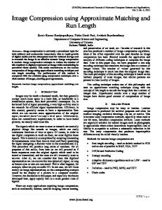
Fig. 1. Edit Mapping between Trees A and B. The tree edit distance between two trees Q and T is the cost of the least costly edit mapping [9]. Definition 6 (Tree Edit Distance): Let Q and T be two ordered labeled trees. The tree edit distance, δ(Q, T ), between Q and T is the cost of the least costly edit mapping, M ⊆ Vǫ (Q) × Vǫ (T ), between the two trees: δ(Q, T ) = min{γ ∗ (M ) | M ⊆ Vǫ (Q) × Vǫ (T ) is an edit mapping} In the unit cost model all nodes have cost 1, and the unit cost tree edit distance [9] is the minimum number of edit operations that transform one tree into the other. Other cost models can be used to tune the tree edit distance to specific application needs, for example, the fanout weighted tree edit distance [21] makes edit operations that change the structure (insertions and deletions of non-leaf nodes) more expensive; in XML, the node cost can depend on the element type. Example 1: Figure 1 illustrates an edit mapping M = {(a1 , b1 ), (a2 , b2 ), (a3 , ǫ), (a4 , b3 ), (ǫ, b4 ), (a5 , b5 ), (a6 , b6 )} between trees A and B. If the cost of all nodes of A and B is 1, γ(a6 , b6 ) = γ(a3 , ǫ) = γ(ǫ, b4 ) = 1; the cost of all other node alignments is zero. M is the least costly edit mapping between A and B, thus the tree edit distance is δ(A, B) = γ ∗ (M ) = 3 (node a6 is renamed, a3 is deleted, b4 is inserted). 4.5 Computing the Tree Edit Distance The fastest algorithms for the tree edit distance use dynamic programming. In this section we discuss the classic algorithm by Zhang and Shasha [9], which recursively decomposes the input trees into smaller units and computes the tree distance bottom-up. The decompositions do not always result in trees, but may also produce forests; in fact, the decomposition rules of Zhang and Shasha [9] assume forests. A forest is recursively decomposed by deleting the root node of the rightmost tree in the forest, deleting the rightmost tree of the forest, or keeping only the rightmost tree of the forest. Figure 4 illustrates the decomposition of the example document H in Figure 2. G
The decomposition of a tree results in the set of all its subtrees and all the prefixes of these subtrees. A prefix is a subforest that consists of the first i nodes of a tree in postorder. Definition 7 (Prefix): Let T be an ordered labeled tree, and ti be the i-th node of T in postorder. The prefix pfx(T, ti ) of T , 1 ≤ i ≤ |T |, is a forest with nodes V ′ = {t1 , t2 , . . . , ti } and edges E ′ = {(tk , tl ) | (tk , tl ) ∈ E(T ), tk ∈ V ′ , tl ∈ V ′ }. A tree with n nodes has n prefixes. The first line in Figure 4 shows all prefixes of example document H. The tree edit distance algorithm computes the distance between all pairs of subtree prefixes of two trees. Some subtrees can be expressed as a prefix of a larger subtree, for example H3 = pfx(H7 , h3 ) in Figure 4. All prefixes of the smaller subtree (e.g., H3 ) are also prefixes of the larger subtree (e.g., H7 ) and should not be considered twice in the tree edit distance computation. The relevant subtrees are those subtrees that cannot be expressed as prefixes of other subtrees. All prefixes of relevant subtrees must be computed. Definition 8 (Relevant Subtree): Let T be an ordered labeled tree and let ti ∈ V (T ). Subtree Ti is relevant iff it is not a prefix of any other subtree: Ti is relevant ⇔ ti ∈ V (T ) ∧ ∀tk , tl (tk ∈ V (T ), tk 6= ti , tl ∈ V (Tk ) ⇒ Ti 6= pfx(Tk , tl )). Example 2: Consider the example trees in Figure 2. The relevant subtrees of G are G2 and G3 , the relevant subtrees of H are H2 , H5 , H6 , and H7 . The decomposition rules for the tree edit distance are given in Figure 3; they decompose the prefixes of two (sub)trees Qm and Tn (qi ≤ qm , tj ≤ tn ). Rule (e) decomposes two general prefixes, (d) decomposes two prefixes that are proper trees (rather than forests), (b) and (c) decompose one prefix when the other prefix is empty, and (a) terminates the recursion. (a) δ(∅, ∅) = 0 (b) δ(pfx(Qm , qi ), ∅) = δ(pfx(Qm , qi−1 ), ∅) + γ(qi , ǫ) (c) δ(∅, pfx(Tn , tj )) = δ(∅, pfx(Tn , tj−1 )) + γ(ǫ, tj ) (d) δ(pfx(Qm , qm ), pfx(Tn , tn )) = min( δ(pfx(Qm , qm−1 ), pfx(Tn , tn )) + γ(qm , ǫ), δ(pfx(Qm , qm ), pfx(Tn , tn−1 )) + γ(ǫ, tn ), δ(pfx(Qm , qm−1 ), pfx(Tn , tn−1 )) + γ(qm , tn )) (e) δ(pfx(Qm , qi ), pfx(Tn , tj )) = min( δ(pfx(Qm , qi−1 ), pfx(Tn , tj )) + γ(qi , ǫ), δ(pfx(Qm , qi ), pfx(Tn , tj−1 )) + γ(ǫ, tj ), δ(pfx(Qm , qi−|Qi | ), pfx(Tn , tj−|Tj | ) + δ(Qi , Tj )) Fig. 3. Decomposition Rules for the Tree Edit Distance.
H
g3 ,a
h7 ,x
4.6 g1 ,b
g2 ,c
h3 ,a h1 ,b
h2 ,d
h6 ,a h4 ,b
h5 ,c
Fig. 2. Example Query G and Document H.
TASM-dynamic
The dynamic programming algorithm for the tree edit distance fills the tree distance matrix td, and the last row of td stores the distances between the query and all subtrees of the document. This yields a simple
5
pfx(H7 , h7 )
pfx(H7 , h6 )
h7
(a)
h6
h3
h3
pfx(H7 , h5 )
(b)
h6
h1 h2 h4 h5
h1 h2 h4 h5
h4 h5
h3
(a, b)
h1 h2 h4 h5
(c)
h6
pfx(H7 , h4 )
h3
(a)
h1 h2 h4 (c)
h5 (a)
(a, b)
h4 h5
pfx(H7 , h2 )
h3
h1 h2
h1 h2
pfx(H7 , h1 )
h1
(a, b)
(a)
(c)
h2
pfx(H5 , h5 )
(c)
pfx(H7 , h3 ) (a, b)
(a) delete rightmost root node (b) delete rightmost tree (c) keep only rightmost tree
h4
pfx(H6 , h5 )
pfx(H2 , h2 )
pfx(H6 , h4 )
pfx(H6 , h6 )
Fig. 4. Decomposing Example Document H into Prefixes. Prefix Distance Matrix pd (only relevant parts are shown): G2 , H2 tj → h2 qi ↓ 0 1 g2 1 1
G2 , H5 tj → h5 qi ↓ 0 1 g2 1 0
G2 , H6 tj → h4 qi ↓ 0 1 g2 1 1
h5 2 1
G3 , H2 tj → qi ↓ 0 g1 1 g2 2 g3 3
G3 , H5 tj → qi ↓ 0 g1 1 g2 2 g3 3
G3 , H6 tj → qi ↓ 0 g1 1 g2 2 g3 3
h5 2 1 0 1
h2 1 1 2 3
h5 1 1 1 2
h4 1 0 1 2
Tree Distance Matrix td:
h6 3 2
G2 , H7 tj → h1 qi ↓ 0 1 g2 1 1
h2 2 2
h3 3 3
h4 4 4
h5 5 4
h6 6 5
h7 7 6
h6 3 2 1 0
G3 , H7 tj → qi ↓ 0 g1 1 g2 2 g3 3
h2 2 1 1 2
h3 3 2 2 1
h4 4 3 3 2
h5 5 4 3 3
h6 6 5 4 3
h7 7 6 5 4
h1 1 0 1 2
G1 G2 G3
H1 H2 H3 H4 H5 H6 H7 1 2 0 1 2 6 0 1 1 3 1 0 2 6 2 3 1 2 2 0 4
R = (H6 , H3 )
Fig. 5. Tree Edit Distance Example.
solution to TASM: compute the tree edit distance between the query and the document, sort the last row of matrix td, and add the k closest subtrees to the ranking. We refer to this algorithm as TASM-dynamic (Algorithm 1). TASM -dynamic is a dynamic programming implementation of the decomposition rules in Figure 3. A matrix td stores the distances between all pairs of subtrees of Q and T . For each pair of relevant subtrees, Qm and Tn , a temporary matrix pd is filled with the distances between all prefixes of Qm and Tn . The distances between all prefixes that are proper subtrees (rather than forests) are saved in td. Note that the prefix pfx(Qm , qi ) is a proper subtree iff pfx(Qm , qi ) = Qi . The ranking, R, is implemented as a max-heap that stores (key, value) pairs: max(R) returns the maximum key of the heap in constant time; push-heap(R, (k, v)) inserts a new element (k, v) in logarithmic time; and pop-heap(R) deletes the element with the maximum key in logarithmic time. Merging two heaps R and R′ yields a new heap of size x = max(|R|, |R′ |), which contains the x elements of R and R′ with the smallest keys. Instead of sorting the distances at the end, Algorithm 1 updates the ranking whenever a new distance between the query and a subtree of the document is available. The input ranking will be used later and is here assumed to be empty. Example 3: We compute TASM-dynamic (k = 2) for query G and document H in Figure 2 (the cost for all nodes is 1, the input ranking is empty). Figure 5 shows the prefix and the tree distance matrixes that are filled by TASM-dynamic. Consider, for example, the prefix distance matrix between G3 and H6 . The matrix is filled column by column, from left to right.
Algorithm 1:
1 2 3 4 5 6 7 8 9 10 11 12 13 14 15 16 17 18 19 20 21 22 23 24 25 26 27 28 29 30 31 32
TASM -dynamic(Q, T, k, R)
Input: query Q, document T , number of matches k, (possibly empty) ranking R, |R| ≤ k Output: top-k ranking of the subtrees of T w.r.t. Q merged with the input ranking R begin td : empty |Q| × |T | matrix; pd : empty (|Q| + 1) × (|T | + 1) matrix; foreach relevant subtree Qm of Q (ascending m) do foreach relevant subtree Tn of T (ascending n) do pd[∅, ∅] ← 0; foreach tj ∈ V (Tn ) (ascending) do pd[∅, tj ] ← pd[∅, tj−1 ] + γ(ǫ, tj ); foreach qi ∈ V (Qm ) (ascending) do pd[qi , ∅] ← pd[qi−1 , ∅] + γ(qi , ǫ); if Qi = pfx(Qm , qi ) ∧ Tj = pfx(Tn , tj ) then pd[qi , tj ] ← min( pd[qi−1 , tj ] + γ(qi , ǫ), pd[qi , tj−1 ] + γ(ǫ, tj ), pd[qi−1 , tj−1 ] + γ(qi , tj )); td[Qi , Tj ] ← pd[qi , tj ]; else pd[qi , tj ] ← min( pd[qi−1 , tj ] + γ(qi , ǫ), pd[qi , tj−1 ] + γ(ǫ, tj ), pd[qi−|Qi | , tj−|Qj | ]+td[Qi , Tj ]) end end if Qm = Q ∧ Tj = pfx(Tn , tj ) then R ← push-heap(R, (td[Qm , Tj ], Tj )); if |R| > k then R ← pop-heap(R); end end end end return R; end
6
The element pd[g2 ][h5 ] stores the distance between the prefixes pfx(G3 , g2 ) and pfx(H6 , g5 ). The upper left element is 0 (Rule (a) in Figure 3); the first column stores the distances between the prefixes of G3 and the empty prefix and is computed with Rule (b); similarly, the elements in the first row are computed with Rule (c); the shaded cells are distances between proper subtrees and are computed with formula (d); the remaining cells use formula (e). The shaded values of pd are copied to the tree distance matrix td. The two smallest distances in the last row are 0 (column 6) and 1 (column 3), thus the top-2 ranking is R = (H6 , H3 ). TASM -dynamic constitutes the state-of-the-art for solving TASM. TASM-dynamic is a fairly efficient approach since it adds a minimal overhead to the already very efficient tree edit distance algorithm. The dynamic programming tree edit distance algorithm uses the result for subtrees to compute larger trees, thus no subtree distance is computed twice. Also, TASM -dynamic improves on the naive solution to TASM (Section 1) by a factor of O(n) in terms of time. However, for each pair of relevant subtrees, Qm and Tn , a matrix of size O(|Qm | × |Tn |) must be computed in this algorithm. As a result, TASM-dynamic requires both the query and the document to be memory resident, leading to a space overhead that is prohibitive even for moderately large documents.
5
P REFIX R ING B UFFER
As will be discussed in Section 6, there is an effective bound on the size of the largest subtrees of a document that can be in the top-k best matches w.r.t. to a query. The key challenge in achieving an efficient solution to TASM is being able to prune large subtrees efficiently and perform the expensive tree edit distance computation on small subtrees only (for which computing the distance to the query is unavoidable). In this section we develop an essential piece of our solution to TASM, which is the prefix ring buffer together with a memory-efficient algorithm for pruning large subtrees. We also prove the correctness of our strategy. The pruning algorithm uses a prefix ring buffer to produce the set of all subtrees that are within a given size threshold τ , but are not contained in a different subtree also within the threshold. This set of subtrees is called the candidate set. Definition 9 (Candidate Set): Given a tree T and an integer threshold τ > 0. The candidate set of T for threshold τ is defined as cand (T, τ ) = {Ti | ti ∈ V (T ), |Ti | ≤ τ, ∀ta ∈ anc(ti ) : |Ta | > τ }. Each element of the candidate set is a candidate subtree. Example 4: The candidate set of the example document D in Figure 6a for threshold τ = 6 is cand (D, 6) = {D5 , D7 , D12 , D17 , D21 }. We stress that the candidate set is not the set of all subtrees smaller than threshold τ , but a subset. If a
D d22 ,dblp d18 ,proceedings
d5 ,article d2 ,auth d4 ,title d7 ,conf
d12 ,article
d21 ,book d17 ,article
d20 ,title
d1 ,John d3 ,X1 d6 ,VLDB d9 ,auth d11 ,title d14 ,auth d16 ,title d19 ,X2 d8 ,Peter d10 ,X3 d13 ,Mike d15 ,X4 (a)
Example Document D
post(D) = ((John, 1), (auth, 2), (X1, 1), (title, 2), (article, 5), (VLDB, 1), (conf, 2), (Peter, 1), (auth, 2), (X3, 1), (title, 2), (article, 5), (Mike, 1), (auth, 2), (X4, 1), (title, 2), (article, 5), (proceedings, 13), (X2, 1), (title, 2), (book, 3), (dblp, 22)) (b)
Postorder Queue of D
Fig. 6. Example Document and Corresponding Postorder Queue. subtree is contained in a different subtree that is also smaller than τ , then it is not in the candidate set. In the dynamic programming approach the distances for all subtrees of a candidate subtree Ti are computed as a side-effect of computing the distance for the candidate subtree Ti . Thus, subtrees of a candidate subtree need no separate computation. 5.1
Memory Buffer
We now discuss how to compute the candidate set given a size threshold τ for a document represented as a postorder queue. Nodes that are dequeued from the postorder queue are appended to a memory buffer (see Figure 7) where the candidate subtrees are materialized. Once a candidate subtree is found, it is removed from the buffer, and its tree edit distance to the query is computed. Postorder Queue: d5 d6 d7 d8 d9 d10 d11 article,5 VLDB,1 conf,2 Peter,1 auth,2 X3,1 title,2 · · · append Memory Buffer: d1 d2 d3 d4 John,1 auth,2 X1,1 title,2
Fig. 7. Incoming Nodes are Appended to the Memory Buffer. The nodes in the memory buffer form a prefix of the document (see Definition 7) consisting of one or more subtrees. All nodes of a subtree are stored at consecutive positions in the buffer: the leftmost leaf of the subtree is stored in the leftmost position, the root in the rightmost position. Each node that is appended to the buffer increases the prefix. New non-leaf nodes are ancestors of nodes that are already in the buffer. They either grow a subtree in the buffer or connect multiple subtrees already in the buffer into a new, larger, subtree.
7
Example 5: The buffer in Figure 7 stores the prefix pfx(D, d4 ) which consists of the subtrees D2 and D4 . When node d5 is appended, the buffer stores pfx(D, d5 ) which consists of a single subtree, D5 . The subtree D5 is stored at positions 1 to 5 in the buffer: position 1 stores the leftmost leaf (d1 ), position 5 the root (d5 ). The challenge is to keep the memory buffer as small as possible, i.e., to remove nodes from the buffer when they are no longer required. We distinguish the nodes in the postorder queue as candidate and noncandidate nodes: candidate nodes belong to candidate subtrees and must be buffered; non-candidate nodes are root nodes of subtrees that are too large for the candidate set. Non-candidate nodes are easily detected since the subtree size is stored with each node in the postorder queue. Candidate nodes must be buffered until all nodes of the candidate subtree are in the buffer. It is not obvious whether a subtree in the buffer is a candidate subtree, even if it is smaller than the threshold, because other nodes appended later may increase the subtree without exceeding τ . 5.2 Simple Pruning A simple pruning approach is to append all incoming nodes to the buffer until a non-candidate node tc is found. At this point, all subtrees rooted among tc ’s children that are smaller than τ are candidate subtrees. They are returned and removed from the buffer. This approach must wait for the parent of a subtree root before the subtree can be returned. In the worst case, this requires to look O(n) nodes ahead and thus a buffer of size O(n) is required. Unfortunately, the worst case is a frequent scenario in data-centric XML with shallow and wide trees. For example, τ = 50 is a reasonable threshold when matching articles in DBLP. However, over 99% of the 1.2M subtrees of the root node of DBLP are smaller than τ ; with the simple pruning approach, all of them will be buffered until the root node is processed. Example 6: Consider the example document in Figure 6. We use the simple approach to prune subtrees with threshold τ = 6. The incoming nodes are appended to the buffer until a non-candidate arrives. The first non-candidate is d18 (represented by (proceedings, 13)), and all nodes appended up to this point (d1 to d17 ) are still in the buffer. The subtrees rooted in d18 ’s children (d7 , d12 , and d17 ) are in the candidate set. They are returned and removed from the buffer. The subtrees rooted in d5 and d21 are returned and removed from the buffer when the root node arrives. 5.3 Ring Buffer Pruning The simple pruning is not feasible for large documents. We now discuss the ring buffer pruning which buffers candidate trees only as long as necessary and
uses a look-ahead of only O(τ ) nodes. This is significant since the space complexity no longer depends on the document size. The size of the ring buffer is b = τ + 1. Two pointers are used: the start pointer s points to the first position in the ring buffer, the end pointer e to the position after the last element. The ring buffer is empty iff s = e, and the ring buffer is full iff s = (e + 1) % b (% is the modulo operator). The number of elements in the ring buffer is (e − s + b) % b ≤ b − 1. Two operations are defined on the ring buffer: (a) remove the leftmost node or subtree, (b) append node tj . Removing the leftmost subtree Ti means incrementing s by |Ti |. Appending node tj means storing node tj at position e and incrementing e. Example 7: The ring buffer (ǫ, d1 , d2 , d3 , d4 , d5 , d6 ), s = 1, e = 0, is full. Removing the leftmost subtree, D5 , with 5 nodes, gives s = 6 and e = 0. Appending node d7 results in (d7 , d1 , d2 , d3 , d4 , d5 , d6 ), s = 6, e = 1. As the buffer is updated, it is possible that at a given point in time consecutive nodes in the buffer form a subtree that does not exist in the document. For example, nodes (d13 , d14 , . . . , d18 ) form a subtree with root node d18 that is different from D18 . We say a subtree in the buffer is valid if it exists in the document. In Section 5.5 we introduce the prefix array to find the leftmost valid subtree in constant time. The ring buffer pruning of a postorder queue of a document T and an empty ring buffer of size τ + 1 is as follows: 1) Dequeue nodes from the postorder queue and append them to a ring buffer until the ring buffer is full or the postorder queue is empty. 2) If the leftmost node of the ring buffer is a nonleaf, then remove it from the buffer, otherwise add the leftmost valid subtree to the candidate set and remove it from the buffer. 3) Go to 1) if the postorder queue is not empty; go to 2) if the postorder queue is empty but the ring buffer is not; otherwise terminate. A non-leaf ti appears at the leftmost buffer position if all its descendents are removed but ti is not, for example, after removing the subtrees D7 , D12 , and D17 , the non-leaf d18 of document D is the leftmost node in the buffer. Example 8: We illustrate the ring buffer pruning on the example tree in Figure 6. The ring buffer is initialized with s = e = 1. In Step 1 nodes d1 to d6 are appended to the ring buffer (s = 1, e = 0, see Figure 8). The ring buffer is full and we move to Step 2. The leftmost valid subtree, D5 , is returned and removed from the buffer (s = 6, e = 0). The postorder queue is not empty and we return to Step 1, where the ring buffer is filled for the next execution of Step 2. Figure 8 shows the ring buffer each time before Step 2 is executed. The shaded cells represent the subtree that is returned in Step 2. Note that in the fourth iteration D17 is returned, not the subtree rooted
8
in d18 , since the subtree rooted in d18 is not valid. Nodes d18 and d22 are non-candidates and they are not returned. After removing d22 the buffer is empty and the algorithm terminates. d2 d1 John,1 auth,2
d3 X1,1
d4 d5 d6 title,2 article,5 VLDB,1
return D5
d7 d8 d9 conf,2 Peter,1 auth,2
d10 X3,1
d11 d5 d6 title,2 article,5 VLDB,1
return D7
d7 d9 d8 conf,2 Peter,1 auth,2
d10 X3,1
d11 d12 d13 title,2 article,5 Mike,1
return D12
d13 d16 d17 d18 d12 title,2 article,5 proc.,13 article,5 Mike,1
return D17
↑e=0 ↑s=1
↑e=5 ↑s=6
↑e=0 ↑s=1
d14 auth,2
d15 X4,1
↑e=5 ↑s=6
d21 d22 d16 d17 d19 d18 book,3 dblp,22 title,2 article,5 proc.,13 X2,1 ↑e=2
skip d18
d20 title,2
return D21
d20 title,2
skip d22
↑s=4
d19 d21 d22 d16 d17 d18 book,3 dblp,22 title,2 article,5 proc.,13 X2,1 ↑e=2
d20 title,2
↑s=5
d22 d21 d16 d17 d18 d19 book,3 dblp,22 title,2 article,5 proc.,13 X2,1 ↑s=1 ↑e=2
Fig. 8. Ring Buffer Pruning Example
5.4 Correctness The ring buffer pruning classifies subtree Ti as candidate or non-candidate based on the nodes already buffered. Lemma 1 proves that this can be done by checking only the τ − |Ti | nodes that are appended after ti and are ancestors of ti : if all of these nodes are non-candidates, then Ti is a candidate tree. The intuition is that a parent of ti that is appended later is an ancestor of both the nodes of ti and the τ − |Ti | nodes that follow ti ; thus the new subtree must be larger than τ . Example 9: Consider example document D of Figure 6a, τ = 6. Fi is the set of τ − |Di | nodes that are appended after di . The subtree D2 is not in the candidate set since F2 = {d3 , d4 , d5 , d6 } contains d5 , which is an ancestor of d2 and a candidate node. D21 is a candidate subtree: |D21 | ≤ τ , F21 = {d22 }, d22 is an ancestor of d21 and |D22 | > τ . (|F21 | < τ − |D21 | since F21 contains the root node d22 which is the last node that is appended.) Lemma 1: Let T be a tree, cand (T, τ ) the candidate set of T for threshold τ , ti the i-th node of T in postorder, and Fi = {tj | tj ∈ V (T ), i < j ≤ i−|Ti|+τ } the set of at most τ − |Ti | nodes following ti in postorder. For all 1 ≤ i ≤ |T | Ti ∈ cand (T, τ ) ⇔ |Ti | ≤ τ ∧ ∀tx (tx ∈ Fi ∩ anc(ti ) ⇒ |Tx | > τ )
(1)
Proof: If |Ti | > τ , then the left side of (1) is false since Ti is not a candidate tree, and the right side
is false due to condition |Ti | ≤ τ , thus (1) holds. If |Ti | ≤ τ we show (tx ∈ Fi ∩ anc(ti ) ⇒ |Tx | > τ ) ⇔ (tx ∈ anc(ti ) ⇒ |Tx | > τ ),
(2)
which makes (1) equivalent to the definition of the candidate set (cf. Definition 9). Case i + τ − |Ti | ≥ |T |: Fi contains all nodes after ti in postorder, thus Fi ∩ anc(ti ) = anc(ti ) and (2) holds. Case i + τ − |Ti | < |T |: (2) holds for all tx ∈ Fi ∩ anc(ti ). If tx ∈ anc(ti ) \ Fi , then tx ∈ / Fi ∩ anc(ti ) and the left side of (2) is true. Since any tx ∈ anc(ti ) \ Fi is an ancestor of all nodes of both Ti and Fi , |Tx | > |Ti | + |Fi | = τ , and (2) holds. As illustrated in Figure 8 the ring buffer pruning removes either candidate subtrees or non-candidate nodes from the buffer. After each remove operation the leftmost node in the buffer is checked. If the leftmost node is a leaf, then it starts a candidate subtree, otherwise it is non-candidate node. Lemma 2: Let T be an ordered labeled tree, cand (T, τ ) be the candidate set of T for threshold τ , ts be the next node of T in postorder after a noncandidate node or after the root node of a candidate subtree, or ts = t1 , and lml (ti ) be the leftmost leaf descendant of the root ti of subtree Ti . ts is a leaf ⇒ ∃Ti : Ti ∈ cand (T, τ ), ts = lml (ti )
(3)
ts is a non-leaf ⇒ ts ∈ {tx | tx ∈ V (T ), |Tx | > τ } Proof: Let N C be the non-candidate nodes of T . (a) ts = t1 : t1 is a leaf, thus t1 ∈ / N C and there is a ti ∈ cand (T, τ ) such that t1 ∈ V (Ti ). There is no node tk < t1 , thus t1 = lml (ti ). (b) ts follows the root node of a candidate subtree Tj : ts is either the parent tk of the root node of Tj or a leaf descendant tl of tk . tk ∈ N C by Definition 9. Since tl is a leaf, tl ∈ / N C and there must be a Ti ∈ cand (T, τ ) such that tl ∈ V (Ti ). We prove tl = lml(ti ) by contradiction: Assume Ti has a leaf tx to the left of tl . As V (Tj ) ∩ V (Ti ) = ∅, tx is to the left of tj , and ta ∈ V (Ti ), the least common ancestor of tl and tx , is an ancestor of tk . This is not possible since |Tk | > τ ⇒ |Ta | > τ ⇒ |Ti | > τ . (c) ts follows a non-candidate node, tx ∈ N C: ts is either the parent tk of tx or a leaf node tl . tk ∈ N C by Definition 9, and there is a Ti ∈ cand (T, τ ) such that tl = lml (ti ) (same rationale as above). Theorem 1 (Correctness of Ring Buffer Pruning): Given a document T and a threshold τ , the ring buffer pruning adds a subtree Ti of T to the candidate set iff Ti ∈ cand (T, τ ). Proof: We show that (1) each node of T is processed, i.e., either skipped or output as part of a subtree, and (2) the pruning in Step 2 is correct,
9
i.e., non-candidate nodes are skipped and candidate subtrees are returned. (1) All nodes of T are appended to the ring buffer: Steps 1 and 2 are repeated until the postorder queue is empty. In each cycle nodes are dequeued from the postorder queue and appended to the ring buffer. All nodes of the ring buffer are processed: The nodes are systematically removed from the ring buffer from left to right in Step 2, and Step 2 is repeated until both the postorder queue and the ring buffer are empty. (2) Let ts be the smallest node of the ring buffer. If ts is the leftmost leaf of a candidate subtree, then the leftmost valid subtree, Ti , is a candidate subtree: Since the buffer is either full or contains the root node of T when Step 2 is executed, all nodes Fi = {tj |tj ∈ V (T ), i < j ≤ i − |Ti | + τ } are in the buffer. If a node tk ∈ Fi is an ancestor of ti , then |Tk | > τ : If ts is the smallest leaf of Tk , then Tk is the leftmost valid subtree which contradicts the assumption; if the smallest leaf of Tk is smaller than ts , then Tk is not a candidate subtree since it contains ts which is the leftmost leaf of a candidate subtree; since tk is an ancestor of ts , the smallest leaf of Tk can not be larger than ts . With Lemma 1 it follows that Ti is a candidate subtree. As Ti is a candidate subtree, with Lemma 2 the pruning in Step 2 is correct. 5.5 Prefix Array The ring buffer pruning removes the leftmost valid subtree from the ring buffer. A subtree is stored as a sequence of nodes that starts with the leftmost leaf and ends with the root node. A node is a (label , size) pair, and in the worst case we need to scan the entire buffer to find the root node of the leftmost valid subtree. To avoid the repeated scanning of the buffer we enhance the ring buffer with a prefix array which encodes tree prefixes (see Definition 7). This allows us to find the leftmost valid subtree in constant time. Definition 10 (Prefix Array): Let pfx(T, tp ) be a prefix of T , and ti ∈ V (T ), 1 ≤ i ≤ p, be the i-th node of T in postorder. The prefix array for pfx(T, tp ) is an integer array (a1 , a2 , . . . , ap ) where ai is the smallest descendant of ti if ti is a non-leaf node, otherwise the largest ancestor of ti in pfx(T, tp ) for which ti is the smallest descendant: ( max{x|x ∈ pfx(T, tp ), lml (x) = ti } if ti is a leaf ai = lml (ti ) otherwise A new node tp+1 is appended to the prefix array (a1 , a2 , . . . , ap ) by appending the integer ap+1 = lml (tp+1 ) and updating the ancestor pointer of its smallest descendant, a(ap+1 ) = ap+1 . A node ti is a leaf iff ai ≥ i. The largest valid subtree in the prefix with a given leftmost leaf ti is (ai , ai+1 , . . . , a(ai ) ) and can be found in constant time. Example 10: Figure 9 shows the prefix arrays of different prefixes of the example tree D and illustrates
the structure of the prefix arrays with arrows. The prefix array for pfx(D, d4 ) is (2, 1, 4, 3). We append d5 and get (5, 1, 4, 3, 1) (the smallest descendant of d5 is d1 , thus a5 = 1 is appended and a1 is updated to 5). Appending d6 gives (5, 1, 4, 3, 1, 6). The largest valid subtree in the prefix pfx(D, d6 ) with the leftmost leaf d1 is (5, 1, 4, 3, 1) (i = 1, ai = 5). pfx(D, d4 ) :
pfx(D, d5 ) : article5
pfx(D, d6 ) : article5
auth2 title4
auth2 title4
auth2 title4
John1 X13
John1 X13
John1 X13 VLDB6
Prefix Array: (2, 1, 4, 3)
Prefix Array: (5, 1, 4, 3, 1)
Prefix Array: (5, 1, 4, 3, 1, 6)
Fig. 9. The Prefix Arrays of Three Prefixes. The pruning removes nodes from the left of the prefix ring buffer such that the prefix ring buffer stores only part of the prefix. The pointer from a leaf to the largest valid subtree in the prefix always points to the right and is not affected. This pointer changes only when new nodes are appended. Theorem 2: The prefix ring buffer pruning for a document with n nodes and with threshold τ runs in O(n) time and O(τ ) space. Proof: Runtime: Each of the n nodes is processed exactly once in Step 1 and in Step 2, then the algorithm terminates. Dequeuing a node from the postorder queue and appending it to the prefix ring buffer in Step 1 is done in constant time. Removing a node (either as non-candidate or as part of a subtree) in Step 2 is done in constant time. Space: The size of the prefix ring buffer is O(τ ). No other data structure is used. 5.6
Algorithm
Algorithm 2 (prb-pruning) implements the ring buffer pruning and computes the candidate set cand (T, τ ) given the size threshold τ and the postorder queue, pq, of document T . The prefix ring buffer is realized with two ring buffers of size b = τ + 1: lbl stores the node labels and pfx encodes the structure as a prefix array. The ring buffers are used synchronously and share the same start and end pointers (s,e). Counter c counts the nodes that have been appended to the prefix ring buffer. After each call of prb-next (Algorithm 3) a candidate subtree is ready at the start position of the prefix ring buffer. It is added to the candidate set and removed from the buffer (Lines 6 and 7). prb-subtree(pfx, lbl, a, b) returns the subtree formed by nodes a to b in the prefix ring buffer. Algorithm 3 is called until the ring buffers are empty.
10
0
Algorithm 2: prb-pruning(pq, τ )
1
0
1 2 3 4 5 6 7 8 9 10 11
Input: postorder queue pq of a document T , threshold τ Output: candidate set cand (T, τ ) begin pfx, lbl: ring buffers of size b = τ + 1; C ← ∅; (pfx, lbl, s, e, c, pq) ← prb-next(pfx, lbl, 1, 1, 0, pq, τ ); while s 6= e do C ← C ∪ {prb-subtree(pfx, lbl, s, pfx[s])}; s ← (pfx[s] + 1) % b; (pfx, lbl, s, e, c, pq) ← prb-next(pfx, lbl, s, e, c, pq, τ ); end return C; end
Algorithm 3 loops until both the postorder queue and the prefix ring buffer are empty. If there are still nodes in the postorder queue (Line 3), they are dequeued and appended to the prefix ring buffer, and the ancestor pointer in the prefix array is updated (Line 8). If the prefix ring buffer is full or the postorder queue is empty (Line 11), then nodes are removed from the prefix ring buffer. If the leftmost node is a leaf (Line 12, c + 1 − (e − s + b) % b is the postorder identifier of the leftmost node), a candidate subtree is returned, otherwise a non-candidate is skipped. Algorithm 3: prb-next(pfx, lbl, s, e, c, pq, τ )
1 2 3 4 5 6 7 8 9 10 11 12 13 14 15 16 17 18 19 20
Input: ring buffers pfx and lbl with start/end pointers s and e, counter c of nodes appended so far, (partially consumed) postorder queue pq of a document T , threshold τ Output: next subtree Ti ∈ cand (T, τ ) begin b ← τ + 1 // ring buffer size while pq 6= ∅ or s 6= e do if pq 6= ∅ then (pq, (λ, size)) ← dequeue(pq); lbl[e] ← λ; pfx[e] ← (++c) − size; if size ≤ τ then pfx[pfx[e] % b] ← c; e ← (e + 1) % b; end if s = (e + 1) % b or pq = ∅ then if pfx[s] ≥ c + 1 − (e − s + b) % b then return (pfx, lbl, s, e, c, pq); else s ← (s + 1) % b; end end end return (pfx, lbl, s, e, c, pq); end
Example 11: Figure 10 illustrates the prefix ring buffer for the example document D in Figure 6. The relative positions in the ring buffer are shown at the top. The small numbers are the postorder identifiers of the nodes. The ring buffers are filled from left to right; overwritten values are shown in the next row.
3
2
5
4
6
John auth X1 title article VLDB 1 2 3 4 5 6
0
1 0
2
3
4
5
6
51 1 2 43 3 4 15 7 6
conf7 Peter8 auth9 X310 title11 article Mike 12 13
6 7 128 8 9 11 812 17 10 10 11 13
proc. X2 title title16 article 17 18 19 20
13 16 15 13 618 21 19 14 15 16 17 19 20
auth14 X415 book21 dblp22
23
24
25
26
Ring Buffer lbl
27
19 122 21
23
24
25
26
27
Prefix Array pfx
Fig. 10. Implementation of the Prefix Ring Buffer.
6
TASM- POSTORDER
We now present a solution for TASM whose space complexity is independent of the document size and, thus, scales well to XML documents that do not fit into memory. Unlike TASM-dynamic (Section 4.6), which requires the whole document in memory, our solution uses the prefix ring buffer and keeps only candidate subtrees in memory at any point in time. We start the section by showing an effective threshold τ for the size of the largest candidate subtree in the document. Then we present TASM-postorder and prove its correctness. 6.1
Upper Bound on Candidate Subtree Size
Recall that solving TASM consists of finding a ranking of the subtrees of the document according to their tree edit distance to a query. We distinguish intermediate and final rankings. An intermediate ranking, R′ = (Ti′1 , Ti′2 , . . . , Ti′k ), is the top-k ranking of a subset of at least k subtrees of a document T with respect to a query Q, the final ranking, R = (Ti1 , Ti2 , . . . , Tik ), is the top-k ranking of all subtrees of document T with respect to the query. We show that any intermediate ranking provides an upper bound for the maximum subtree size that must be considered (Lemma 4). The tightness of such a bound improves with the quality of the ranking, i.e., with the distance between the query and the lowest ranked subtree. We initialize the intermediate ranking with the first k subtrees of the document in postorder. Lemma 5 provides bounds for the size of these subtrees and their distance to the query. The ranking of the first k subtrees provides the upper bound τ = |Q|(cQ + 1) + kcT for the maximum subtree size that must be considered (Theorem 3), where cQ and cT denote the maximum costs of any node in Q and the first k nodes in T , respectively (cf. Section 4.4). Note that this upper bound τ is independent of size and structure of the document Lemma 3: Let Q and T be ordered labeled trees, then |T | ≤ δ(Q, T ) + |Q|. Proof: We show |T | − |Q| ≤ δ(Q, T ). True for |T | ≤ |Q| since δ(Q, T ) ≥ 0. Case |T | > |Q|: At least |T | − |Q| nodes must be inserted to transform Q into T . The cost of inserting a new node, tx , into T is γ(ǫ, tx ) = cst(tx ) ≥ 1.
11
Lemma 4 (Upper Bound): Let R′ = (Ti′1 , Ti′2 , . . . , Ti′k ) be any intermediate ranking of at least k subtrees of a document T with respect to a query Q, and let R be the final top-k ranking of all subtrees of T , then ∀Tij (Tij ∈ R ⇒ |Tij | ≤ δ(Q, Ti′k ) + |Q|). Proof: |Tij | ≤ δ(Q, Tij ) + |Q| follows from Lemma 3. We show ∀Tij (|Tij | ∈ R ⇒ δ(Q, Tij ) ≤ δ(Q, t′ik )) by contradiction: Assume a subtree Tij ∈ R, δ(Q, Tij ) > δ(Q, Ti′k ). Then by Definition 1 also Ti′k ∈ R; if Ti′k ∈ R, then also all other Ti′l ∈ R′ are in R, / R′ (since δ(Q, Tij ) > δ(Q, Ti′k )) but i.e., R′ ⊆ R. Tij ∈ ′ Tij ∈ R, thus R ∪ {Tij } ⊆ R. This contradicts |R| = k. Lemma 5 (First Ranking): Let Q and T be ordered labeled trees, k ≤ |T |, cQ and cT be the maximum costs of a node in Q and the first k nodes in T , respectively, ti be the i-th node of T in postorder, then for all Ti , 1 ≤ i ≤ k, the following holds: |Ti | ≤ k ∧ δ(Q, Ti ) ≤ |Q|cQ + kcT . Proof: Let qi be the i-th node of Q in postorder, and lml (ti ) the leftmost leaf of Ti . The nodes of a subtree have consecutive postorder numbers. The smallest node is the leftmost leaf, the largest node is the root. Since the leftmost leaf of Ti , 1 ≤ i ≤ k, is larger or equal 1 and the root is at most k, the subtree size is bound by k. The distance between the query and the document is maximum if the edit mapping is empty, i.e., all nodes of Q arePdeleted and all nodes of Ti are inserted: δ(Q, Ti ) ≤ qi ∈V (Q) γ(qi , ǫ)+ P ti ∈V (Ti ) γ(ǫ, ti ) ≤ |Q|cQ + kcT since γ(qi , ǫ) ≤ cQ , γ(ǫ, ti ) ≤ cT , and |Ti | ≤ k. The three lemmas above are the elements for our main result in this section:
buffer (Lines 5 and 19), it is processed and removed (Line 18). If an intermediate ranking is available (i.e., |R| = k) the upper bound τ ′ provided by the intermediate ranking (see Lemma 4) may be tighter than τ . Only subtrees of Ti that are smaller than τ ′ must be considered. The subtrees of Ti (including Ti itself) are traversed in reverse postorder, i.e., in descending order of the postorder numbers of their root nodes. If a subtree of Ti is below the size threshold τ ′ , then TASM -dynamic is called for this subtree and the ranking R is updated. All subtrees of the processed subtree are skipped (Line 13), and the remaining subtrees of Ti are traversed in reverse postorder. Algorithm 4:
1 2 3 4 5 6 7 8 9 10 11 12 13 14 15 16 17 18 19
Theorem 3 (Maximum Subtree Size): Let query Q and document T be ordered labeled trees, cQ and cT be the maximum costs of a node in Q and the first k nodes in T , respectively, R = (Ti1 , Ti2 , . . . , Tik ) be the final top-k ranking of all subtrees of T with respect to Q, then the size of all subtrees in R is bound by τ = |Q|(cQ + 1) + kcT : ∀Tij (Tij ∈ R ⇒ |Tij | ≤ |Q|(cQ + 1) + kcT )
(4)
Proof: |T | < k: (4) holds since |Tij | ≤ |T | < k ≤ |Q|(cQ +1)+kcT . |T | ≥ k: According to Lemma 5 there is an intermediate ranking R′ = (Ti′1 , Ti′2 , . . . , Ti′k ) with δ(Q, Ti′k ) ≤ |Q|cQ + kcT , thus δ(Q, Tij ) ≤ |Q|cQ + kcT (Lemma 4) and |Tij | ≤ |Q|cQ + kcT + |Q| (Lemma 3) for all subtrees Tij ∈ R. 6.2 Algorithm TASM -postorder
(Algorithm 4) uses the upper bound τ (see Theorem 3) to limit the size of the subtrees that must be considered, and the set of candidate subtrees, cand (T, τ ), is computed using the prefix ring buffer proposed in Section 5. When a candidate subtree Ti ∈ cand (T, τ ) is available in the prefix ring
20 21 22
TASM - postorder(Q, pq, k)
Input: query Q, postorder queue pq of a document T , result size k Output: top-k ranking of the subtrees of T w.r.t. Q begin R : empty max-heap; // top-k ranking τ ← |Q|(cQ + 1) + kcT ; τ ′ ← τ ; pfx, lbl: ring buffers of size b = τ + 1; (pfx, lbl, s, e, c, pq) ← prb-next(pfx, lbl, 1, 1, 0, pq, τ ); while s 6= e do r ← pfx[s] // candidate subtree root while r ≥ pfx[pfx[s] % b] do Ti ← prb-subtree(pfx, lbl, pfx[r % b], r % b); if |R| = k then τ ′ = min(τ, max(R) + |Q|); if |R| < k ∨ |Ti | < τ ′ then R ← TASM - dynamic(Q, Ti , k, R); r ← r − |Ti |; else r ← r − 1; end end s ← (pfx[s] + 1) % b; (pfx, lbl, s, e, c, pq) ← prb-next(pfx, lbl, s, e, c, pq, τ ); end return R; end
Theorem 4 (Correctness): Given a query Q, a document T , and k ≤ |T |, TASM-postorder (Algorithm 4) computes the top-k ranking R of all subtrees of T with respect to Q. Proof: If no intermediate ranking is available, all subtrees within size τ = |Q|(cQ + 1) + kcT are considered. The correctness of τ follows from Theorem 3. Subtrees of size τ ′ = min(τ, max(R) + |Q|) and larger are pruned only if an intermediate ranking with k subtrees is available. Then the correctness of τ ′ follows from Lemma 4. Theorem 5 (Complexity): Let Q and T be ordered labeled trees, m = |Q|, n = |T |, k ≤ |T |, cQ and cT be the maximum costs of a node in Q and the first k nodes in T , respectively. Algorithm 4 uses O(m2 n) time and O(m2 cQ + mkcT ) space. Proof: The space complexity of Algorithm 4 is dominated by the call of TASM-dynamic(Q, Ti , k, R)
12
in Line 12, which requires O(m|Ti |) space. Since |Ti | ≤ τ = m(cQ + 1) + kcT , the overall space complexity is O(m2 cQ + mkcT ). The runtime of TASM -dynamic(Q, Ti , k, R) is O(m2 |Ti |). τ is the size of the maximum subtree that must be computed. There can be at most n/τ subtrees of size τ in the document and the runtime complexity is O( nτ m2 τ ) = O(m2 n). The space complexity is independent of the document size. cQ and cT are typically small constants, for example, cQ = cT = 1 for the unit cost tree edit distance, and the document is often much larger than the query. For example, a typical query for an article in DBLP has 15 nodes, while the document has 26M nodes. If we look for the top 20 articles that match the query using the unit cost edit distance, TASM -postorder only needs to consider subtrees up to a size of τ = 2|Q| + k = 50 nodes, compared to 26M in TASM-dynamic. Note that for TASM-postorder a subtree with 50 nodes is the worst case, whereas TASM -dynamic always computes the distance between the query and the whole document with 26M nodes. 6.3 Pushing Pruning into TASM-dynamic TASM -postorder calls TASM -dynamic for document subtrees that can not be pruned. TASM-dynamic computes the distances between the query and all subtrees. In this section we apply our pruning rules inside TASM-dynamic and stop the execution early, i.e., before all matrixes are filled. We leverage the fact that the ranking improves during the execution of TASM -dynamic, giving rise to a tighter upper bound for the maximum subtree size. We refer to TASM-dynamic with pruning as TASM -dynamic+ (Algorithm 5). The pruning is inserted between Lines 7 and 8 of TASM-dynamic, all other parts remain unchanged. Whenever the pruning condition holds, the unprocessed columns of the current prefix distance matrix (pd) are skipped.
Algorithm 5:
1 7
8 28 31 32
TASM -dynamic+ (Q, T, k, R)
Input: query Q, document T , number of matches k, (possibly empty) ranking R, |R| ≤ k Output: top-k ranking of the subtrees of T w.r.t. Q merged with the input ranking R begin ··· foreach tj ∈ V (Tn ) (ascending) do if |R| = k ∧ | pfx(Tn , tj )| > max(R) + |Q| then goto line 28; // exit inner loop end pd[∅, tj ] ← pd[∅, tj−1 ] + γ(ǫ, tj ) ··· end ··· return R end
Example 12: We compute TASM-dynamic+ (k = 2) for the query G and the document H in Figure 2 (the cost for all nodes is 1, the input ranking is empty). The gray values in the prefix and tree distance matrixes in Figure 5 are the values that TASM-dynamic+ does not need to compute due to the pruning. Before column h5 in the prefix distance matrix between G3 and H7 is computed, R = ((H6 , 0), (H3 , 1)) and the pruning condition holds (|R| = 2, | pfx(H7 , h5 )| = 5, max(R) = 1, |G| = 3). The columns h5 , h6 , and h7 can be skipped and the distances δ(G1 , H7 ) and δ(G3 , H7 ) need not be computed. Theorem 6 (Correctness of TASM-dynamic+ ): Given a query Q, a document T , k ≤ |T |, and a ranking R of at most k subtrees with respect to the query Q, TASM -dynamic+ (Algorithm 5) computes the top-k ranking of the subtrees in the ranking R and all subtrees of document T with respect to the query Q. Proof: Without pruning the algorithm computes all distances between the query Q and the subtrees of document T . Whenever a new distance is available, the ranking is updated and the final ranking R is correct. If the pruning condition holds for a prefix pfx(Tn , tj ) of the relevant subtree Tn , then column tj of the prefix distance matrix pd, all following columns of pd, and some values of the tree distance matrix td will not be computed. We need to show that (1) we do not miss a subtree that should be in the final ranking R, and (2) the values of td that are not computed are not needed later. (1) Let pi = pfx(Tn , ti ) be a prefix of Tn . We need to show ∀pi (ti ≥ tj ⇒ pi ∈ / R): If pi is not a subtree then pi ∈ / R (Definition 1). If pi is a subtree, pi ∈ / R follows from Lemma 4: Since the pruning condition requires |R| = k, an intermediate ranking (Ti′1 , Ti′2 , . . . , Ti′k ) is available and δ(Q, Ti′k ) = max(R); thus a subtree Ti can not be in the final ranking if |Ti | > max(R) + |Q|. | pfx(Tn , tj )| > max(R) + |Q| (pruning condition) and pi ≥ | pfx(Tn , tj )| for ti ≥ tj , thus pi ∈ / R. (2) Let pd be the prefix distance matrix between two relevant subtrees Qm and Tn . A column tj of pd can be computed if (a) all columns of pd to the left of tj are filled, and (b) all prefix distance matrixes between Tn and the relevant subtrees Qi of Qm (Qi 6= Qm ) are filled up to column tj (follows from the decomposition rules in Figure 3). (a) holds since the columns are computed from left to right, and columns to the right of a pruned column are pruned as well; (b) holds since the prefix distance matrixes for the subtrees Qi are computed before pd, and if the pruning condition holds for column tj in the matrix of a subtree Qi , then it also holds for column tj in the matrix of Qm (in the pruning condition, | pfx(Tn , tj )| and |Q| do not change and max(R) can not increase). We adapt TASM-postorder (Algorithm 4) by replacing TASM-dynamic with TASM-dynamic+ in Line 12 and use this version of the algorithm in our experimental evaluation.
13
7.1
time (seconds)
1e3
1e2 pos, |Q|=64 dyn, |Q|=8 dyn, |Q|=4 pos, |Q|=8 pos, |Q|=4
1e1
1e0 112
(a)
224 448 896 document size (MB)
1792
Varying Document Size; k = 5.
time (seconds)
1e3
1e2 pos, T:1792MB dyn, T:224MB dyn, T:112MB pos, T:224MB pos, T:112MB
1e1
1e0 4
8
(b)
16 32 query size (nodes)
64
Varying Query Size; k = 5.
300
time (seconds)
250
dyn, T:224MB dyn, T:112MB pos, T:224MB pos, T:112MB
200 150 100 50 0 1e0
1e1
(c)
1e2 k
1e3
1e4
Varying k; |Q| = 16.
Fig. 11. Execution Times for Varying Sizes of Document, Query and k.
7
E XPERIMENTAL VALIDATION
In this section we experimentally evaluate our solution. We study the scalability of TASM-postorder using realistic synthetic XML datasets of varying sizes and the effectiveness of the prefix ring buffer pruning on large real world datasets. All algorithms were implemented as single-thread applications in Java 1.6 and run on a dual-core AMD64 server. A standard XML parser was used to implement the postorder queues (i.e., parse and load documents and queries). In all algorithms we use a dictionary to assign unique integer identifiers to node labels (element/attribute tags as well as text content). The integer identifiers provide compression and faster node-to-node comparisons, resulting in overall better scalability.
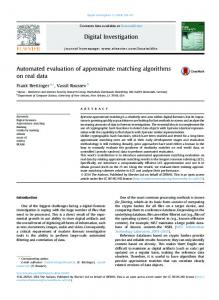
Scalability
We study the scalability of TASM-postorder using synthetic data from the standard XMark benchmark [25], whose documents combine complex structures and realistic text. There is a linear relation between the size of the XMark documents (in MB) and the number of nodes in the respective XML trees; the height does not vary with the size and is 13 for all documents. We used documents ranging from 112MB and 3.4M nodes to 1792MB and 55M nodes. The queries are randomly chosen subtrees from one of the XMark documents with sizes varying from 4 to 64 nodes. For each query size we have four trees. We compare TASM -postorder against the state-of-the-art solution, TASM -dynamic (Section 4.6) implemented using the tree edit distance algorithm by Zhang and Shasha [9]. Execution Time: Figure 11a shows the execution time as a function of the document size for different query sizes |Q| and fixed k = 5. Similarly, Figure 11b shows the execution time versus query size (from 4 to 64 nodes) for different document sizes |T | and fixed k = 5. The graphs show averages over 20 runs. The data points missing in the graphs correspond to settings in which TASM-dynamic runs out of main memory (4GB). As predicted by our analysis (Section 6), the runtime of TASM-postorder is linear in the document size. TASM-postorder scales very well with both the document and the query size, and can handle very large documents or queries. In contrast, TASM -dynamic runs out of memory for trees larger than 500MB, except for very small queries. Besides scaling to much larger problems, TASM-postorder is also around four times faster than TASM-dynamic. Figure 11c shows the impact of parameter k on the execution time of TASM-postorder (|Q| = 16). As expected, TASM-dynamic is insensitive to k since it always must compute all subtrees. TASM-postorder, on the other hand, prunes large subtrees, and the size of the pruned subtrees depends on k. As the graph shows (observe the log-scale on the x-axis), TASM -postorder scales extremely well with k: an increase of 4 orders of magnitude in k results only in doubling the low runtime. Figure 12 compares the execution times of TASM -dynamic+ and TASM -dynamic. TASM -dynamic+ is, on average, 45% faster than TASM-dynamic since distance computations to large subtrees are pruned. Main Memory Usage: Figure 13 compares the main memory usage of TASM-postorder and TASM-dynamic for different document sizes. The graph shows the average memory used by the Java virtual machine over 20 runs for each query and document size. (The memory used by the virtual machine depends on several factors and is not constant across runs.) We omit the plots for other query sizes since they follow the same trend as the ones shown in Figure 13: the memory requirements are independent of
14
1e3
pos xq-twig SAX
time (seconds)
time (seconds)
1e3
1e2
1e1
dyn, |Q|=8 dyn+, |Q|=8 dyn, |Q|=4 dyn+, |Q|=4
1e0 33
Fig. 12.
66 112 224 document size (MB)
TASM -dynamic+
vs. TASM-dynamic; k = 5.
4e3 3GB memory (MB)
1e3
8MB
1e1
dyn, |Q|=16 dyn, |Q|=4 pos, |Q|=16 pos, |Q|=4
1e0 112
224 448 896 document size (MB)
1e1
1e0 448
the document size for TASM-postorder and linearly dependent on the document size for TASM-dynamic. In both cases the experiment agrees with our analysis. The missing points in the plot correspond to settings for which TASM-dynamic runs out of memory (4GB). The difference in memory usage is remarkable: while for TASM-postorder only small subtrees need to be loaded to main memory, TASM-dynamic requires data structures in main memory that are much larger than the document itself.
1e2
1e2
1792
Fig. 13. Memory Usage as a Function of the Document Size; k = 5. 7.2 TASM-postorder vs. XQuery In order to give a feel for the overall performance of TASM-postorder we compare its execution time against XQuery-based twig queries that find exact matches of the query tree. This can be seen as a very restricted solution to TASM and is the special case when k = 1 and an identical copy of the query exists in the document. For example, query G in Figure 2 can be expressed as follows: for $v1 in //a[count(node()) eq 2] let $v2:=$v1/b[1][not (node())], $v3:=$v1/c[1][not (node())] where $v2