Efficient Triangulation of Point Clouds Using Floater Parameterization Tim Volodine Dirk Roose Denis Vanderstraeten Report TW 385, January 2004
Katholieke Universiteit Leuven Department of Computer Science Celestijnenlaan 200A – B-3001 Heverlee (Belgium)
Efficient Triangulation of Point Clouds Using Floater Parameterization Tim Volodine Dirk Roose Denis Vanderstraeten Report TW 385, January 2004
Department of Computer Science, K.U.Leuven
Abstract A method for constructing 3D triangulations of scanned 3D point data has been introduced by Floater et al.. First, a 2D parameterization of the points is computed and triangulated. The 3D triangulation is obtained directly from the 2D triangulation. This method requires an ordered boundary of the point cloud, and the computation of the 2D parameterization requires the solution of a large linear system. In this paper we present an efficient boundary estimation algorithm, and we compare various approaches to solve the linear system. We show that, after an appropriate reordering of the matrix, the system can be solved very efficiently using a direct sparse solver.
Keywords : parameterization, surface reconstruction, triangulation. CR Subject Classification : G.1.3, I.3.5. AMS(MOS) Classification : Primary : 65Y20, 65D18 Secondary : 65F50, 65F05, 65M50.
Efficient Triangulation of Point Clouds Using Floater Parameterization Tim Volodine∗
Dirk Roose∗
Denis Vanderstraeten†
January 21, 2004
Abstract A method for constructing 3D triangulations of scanned 3D point data has been introduced by Floater et al.. First, a 2D parameterization of the points is computed and triangulated. The 3D triangulation is obtained directly from the 2D triangulation. This method requires an ordered boundary of the point cloud, and the computation of the 2D parameterization requires the solution of a large linear system. In this paper we present an efficient boundary estimation algorithm, and we compare various approaches to solve the linear system. We show that, after an appropriate reordering of the matrix, the system can be solved very efficiently using a direct sparse solver.
1 Introduction The problem of surface reconstruction, and in particular triangulation of unorganized point clouds is an active area of research. We state the reconstruction problem as an interpolation problem: given a set of points in R3 , construct a triangular mesh which interpolates in all the given points and in this way defines a piecewise linear interpolating surface. Many methods for this problem have been developed over the past years. In general we can distinguish four main approaches. • Implicit methods. These methods usually involve the computation of some signed distance function, whose zero isosurface is considered to be the reconstructed implicit surface. The signed distance function is typically constructed by adding extra non-surface points and estimating their distance to the surface. The reconstructed implicit surface can be used to generate a mesh, by means of an iso-surfacing algorithm such as Marching Cubes. An implicit ray-tracer can be used to visualize the surface directly. The reconstructed surface is usually smoother than a triangulation of the data points, ∗ e-mail: † e-mail:
{timv,dirkr}@cs.kuleuven.ac.be
[email protected]
1
which makes this method suitable for noisy data. Algorithms using this approach include [23], [22] for unorganized point-clouds, and [10] which exploits structural properties of the point data. Another implicit algorithm [21] searches for a surface which minimizes the global distance function to the data set. Starting with an initial guess of an enclosing implicit surface, the level set method is applied to deform the initial surface based on a convection model. This requires the solution of time dependent PDEs. The resulting surface is smoother than linear. In Carr et al. [9] radial basis functions are fitted to the signed distance function, the surface is then defined as the locus of all points where the radial basis function is zero. • 3D Delaunay-triangulation based techniques. This approach uses the Delaunay tetrahedrization and a filtering strategy for constructing a triangular mesh as a subset of the Delaunay triangulation. These methods are often robust and have proven reconstruction properties concerning sampling density and quality guarantees. However they tend to be costly, because of the computation of the Delaunay triangulation or its dual Voronoi diagram. Boissonnat [8] uses a method which successively removes tetrahedra from a Delaunay tetrahedrization of the points. In [15] the notion of an α − shape is described as a generalization of the convex hull of a point set. For example the 0-shape is the point cloud itself, and the ∞-shape is the convex hull of the points. The α -shape is usually extracted from the Delaunay-tetrahedrization, and for a suitable α -value it gives a visually acceptable piecewise linear approximation of the surface. The crust algorithm [2] uses a 3D Voronoi diagram of the sample points. The power crust algorithm [4] uses a weighted version of the 3D Voronoi diagram, called the power diagram. Another similar algorithm is the Cocone algorithm [3], which is a simplified version of the crust-algorithm and tends to be faster. To address the slowness and bad scalability of the Delaunay-based algorithms, Dey et al developed a version of the Cocone algorithm called Super Cocone [14]. Significant speedups are obtained by avoiding the computation of the global Delaunay triangulation. This is done by partitioning the points into an octree, and applying the Cocone algorithm to each of the clusters. Some hybrid algorithms were also developed, which use both the α -shapes and implicitly defined distance function [6]. • Local triangulations, also called advancing front algorithms. Bernardini et al [7] introduced a Ball-Pivoting Algorithm for reconstructing a triangular mesh from a point cloud. A ball of given radius is rolled over the points and each three points form a triangle if the ball touches them without containing 2
any other point. This simple and fast algorithm was used to construct a mesh of the Michelangelo’s Florentine Pieta which contains 7.2M points. However this algorithm uses an approximation of the normal at each data point, and requires multiple passes for unevenly sampled surfaces. Another local algorithm is described in [19]. • Meshless parameterization. In this approach, introduced by Floater in [18], the 3D triangulation is obtained by triangulating the parameterized points in 2D and lifting this triangulation into 3D. Large systems of linear equations have to be solved to compute the parameterization. However, this approach is restricted by the requirement that the point cloud must be homeomorphic to a disc, and a valid boundary has to be computed for each point cloud. In this paper we describe a simple algorithm for triangulating point clouds which are homeomorphic to a disc, based on the Floater parameterization of the points. First, we extend and automate the boundary extraction as proposed in [18]. Second, we show how to efficiently solve the linear system to obtain a global parameterization of the points. Finally we evaluate the results and outline the limitations of this approach.
2 Floater Approach 2.1
Parameterization
Floater has proposed a method [16], based on convex combination mapping, for creating global parameterizations of triangulated surfaces. In [18], this method has been extended to parameterize point clouds directly, without any intermediate triangulation. The algorithm is based on a method proposed by Tutte [27] for making straight line drawings of planar graphs. The method of Floater maps the points into some convex parameter domain in the plane, by solving a global system of linear equations. The equations arise from requiring that each interior parameter point is a convex combination of its neighbors. This can be stated as a linear equation for each interior parameter point u i ∈ R2 : ui =
∑ λi j u j
, i = 1..m .
j∈Ni
where Ni is a set of indices of neighboring points, m is the number of interior points and λi j are the weights, which can be chosen arbitrarily, but have to satisfy the following equations ( λi j ≥ 0 for j ∈ Ni and zero elsewhere, ∑ j∈N λi j = 1. i
The parameter points ui , corresponding to the boundary points of the point cloud, are not a convex combination of other points. Fixing these points on some 3
convex curve in the parameter domain allows to solve the parameter values of the remaining interior points. Let {um+1 , ..., uN } be the boundary points, with N the total number of points. Then we have to solve the linear system
1 −λ21 .. .
−λ12 1
−λm1 −λm2
. . . −λ1m . . . −λ2m .. .. . . ... 1
u1 u2 .. . um
=
∑Nj=m+1 λ1 j u j ∑Nj=m+1 λ2 j u j .. . ∑Nj=m+1 λm j u j
.
(1)
Most of the weights λi j are zero, because the neighborhoods are limited in size, hence the system is typically very sparse. Two important ingredients of this method are the choice of the neighborhoods and the weights λi j . There are various possibilities for choosing neighborhoods: e.g ball neighborhood, k-nearest neighbors, Delaunay neighborhood see Figure 1(b). Some choices for the weights are uniform, weighted, reciprocal distance weights, shape-preserving weights and recently mean-value weights [17]. The latter are a smooth extension of the shape-preserving weights, see section 4.1.
2.2
Overview of the Algorithm
The algorithm consists of three main steps: • Boundary extraction. To parameterize a point cloud using Floater parameterization, it is necessary to have a closed boundary, which can be mapped onto a convex curve in the plane, such that the overall parameterization is homeomorphic to a disc. Some boundary extraction methods have been proposed in [13], [20]. We use a classical approach to solve this problem by using the largest angle criterion for classification of the points, as described in the next section. • Construction of the parameterization matrix. Each row in the matrix corresponds to one data point and contains non-zero elements, weights, for each point in the neighborhood around that point. There are several possibilities for the choice of neighborhoods and weights [16]. In this paper we use the mean value coordinates [17] for the weights in conjunction with Delaunay neighborhoods. • Solution of the linear system constructed in the previous step. Here either an iterative method, or a direct sparse solver can be used. We compare both approaches and show that in most cases it is possible to efficiently use a direct sparse LU-decomposition, because of the special structure of the system.
4
vj+1 vi
ô
áij áij-1
vj
vj-1 (a)
(b)
(c)
Figure 1: (a) open angle criterion (b) ball, knn and Delaunay neighborhoods (c) mean value weights
3 Boundary Extraction 3.1
Boundary Detection
For a compact surface S with boundary, we can distinguish interior points from the boundary points as follows. An interior point has a neighborhood homeomorphic to the open disc. A boundary point, on the other hand, has a neighborhood homeomorphic to the half-disc. To detect the boundary points, we slightly modify the approach presented in [18]. A point is considered to be a boundary point if its neighborhood has an opening-angle τ larger than a given minimum angle τ min (τmin = 160° in our implementation), after projection on the least-squares plane. With this criterion the central point in Figure 1(a) is classified as a boundary point.
3.2
Clustering Boundary Points
After all data points are processed, the resulting boundary points usually form a collection of clusters. Often there are some misclassifications due to small holes in the point cloud, noise, or due to under-sampled large curvature regions. We developed a clustering heuristic which allows to extract the largest cluster and consider it to be the real boundary, see Figure 2(a). For the clustering algorithm, some tolerance ξ is supplied, which is a percentage of the length of the bounding box diagonal D, e.g. for the dragon-model in Figure 2(a) we use ξ = 5%. The algorithm takes two parameters ξ and k (k = 10 in our implementation) and follows a region growing approach. 1. In a preprocessing step: all boundary points are extracted. 2. The local density around each boundary point is estimated. This is done by assuming that the density is proportional to the number of boundary points in the sphere of radius ξ D, centered around that point. Until all points are processed do 5
3. Choose the unprocessed point p with highest density and designate it as a starting point for a new cluster C. 4. Select k nearest neighbor points of p, and append them to the cluster C, if their distance to p does not exceed ξ percent of the bounding box diagonal. Mark p as processed. 5. Redefine p as any unprocessed point in C and proceed with step 4 until all points in cluster C are processed. We try to maximize the number of clusters, by selecting points according to descending local density, since isolated (possibly misclassified) points tend to have small density. After executing this algorithm on the HALF DRAGON point cloud we obtain 63 clusters as shown in Figure 2(a). The largest cluster (red cluster in Figure 2(a)) defines the outer boundary, the small clusters represent noise artifacts and are discarded.
3.3
Ordering the Boundary
It is important to order the boundary points, to make a correct parameterization. This is in fact a 3D curve reconstruction problem. In [18] the 1D-analogue of the Floater parameterization is used to solve this problem. However when using univariate Floater parameterization we need to fix a start point and an end point of the curve. In our case we have a boundary loop, which doesn’t have an obvious start or end points. In [18], it is suggested to separate the points by a plane in two parts, and to order each part by the univariate Floater parameterization. However, this approach is not flexible and it is difficult to automate. Sometimes it is not easy to find a suitable dividing plane. Therefore we use a region-growing approach as in the clustering algorithm, to divide the loop in two segments. The input of the algorithm is a set of unordered boundary points, which form a loop. The output are two connected segments of approximately equal size, which are disjunct except for the start and end points. 1. first a random seed point is selected; 2. afterwards k nearest neighbors are appended to the segment, starting with k=3; 3. if all nearest neighbor points are already in the segment, k is incremented; 4. this process is repeated until the number of points in the segment is larger than l/2 (where l is the total number of boundary points). After executing the above algorithm we obtain a connected segment of unordered points, which is the first segment. The second segment is constructed in the same fashion, except that it is initialized with the last point appended to 6
1
0 seed point
s1_start s2_end s1_end s2_start
0
1
(a)
(b)
Figure 2: (a) half-dragon point cloud (≈ 256 000 points). (b) the points in the largest cluster are split in two segments, each of which is parameterized on the [0, 1] interval, to obtain an ordering.
the first segment, which is called segment1 end, and is at the same time also segment2 start. After all remaining points are appended to the second segment, the last point appended is called segment2 end, which is also segment1 start. Each of the two resulting segments are then parameterized by the 1D analogue of the Floater parameterization, and stitched together to obtain a full closed boundary loop. This loop can further be mapped onto any convex curve in the plane. In this paper we mostly use a circle, with a mapping by chord length. The ordering algorithm is also illustrated in Figure 2(b). Figure 3(a) shows a somewhat more complex example of boundary extraction and ordering.
4 Computing the Parameterization 4.1
Calculation of the Weights
For each interior point p a knn-neighborhood is computed, which is then projected on its least-squares plane. The Delaunay neighborhood is extracted from the Delaunay triangulation of the projected points. Consequently the mean value weights are computed by the formula [17]
λi j =
wi j ∑k∈Ni wik
, wi j =
tan(αi j−1 /2) + tan(αi j /2) kv j − vi k2
7
(2)
(a)
(b)
Figure 3: (a) nontrivial boundary ordering of the FACE STRIP model (b) corresponding mesh with ≈ 60 000 points. with angles αi j as shown on Figure 1(c) and the Delaunay neighbors ordered in anti-clockwise fashion. The weights can be computed very efficiently using s 1 − cos(α ) , 0≤α ≤π , tan(α /2) = (3) 1 + cos(α ) where the cosine can be expressed as a dot product.
4.2
Solution of the Linear System
The resulting large linear system in Equation 1 is unsymmetric and very sparse. When using Delaunay neighborhoods for example, the parameterization matrix has on average only 7 non-zero elements per row. For a 30 000 points model this implies that 0.02% of the matrix entries are non-zero. Traditionally the resulting large sparse system is solved using an iterative solver, such as Gauss-Seidel or Krylov subspace methods (e.g. BICGSTAB) [24], [18]. When a direct solution method (i.e. LU-factorization) is used, the fill-in (extra non-zero elements in the L and U factors) can be substantial. However, fill-in can be reduced if the matrix is first re-ordered (using row and column permutations). Our experiments indicate that the matrices arising in this method can be reordered effectively, so that a direct sparse LU-decomposition becomes very efficient. Figure 4(a) shows the matrix of the linear system as obtained from the bunny model. In Figure 4(b) the same matrix is reordered using the reverse CuthillMcKee algorithm. For LU-decomposition, the minimum degree reordering is more suitable, because it results in less fill-in (Figure 4(c)). In fact, the linear system we have to solve has the properties of systems arising from finite element methods. For such systems the minimum degree reordering has been found to work
8
extremely well. This reordering technique, more specifically approximate minimum degree reordering, is implemented in the AMD library [5], and is part of the UMFPACK solver. The UMFPACK [11] solver is a general purpose direct sparse solver for unsymmetric systems, which is based on the Unsymmetric-pattern Multi-Frontal method. The Floater system is usually unsymmetric, depending on the choice of weights, but in most cases it has a near-symmetrical structure. This fact is also exploited in UMFPACK by using the so-called symmetrical strategy, which results in faster column pre-ordering. In addition the matrix is also diagonally dominant, contributing to the speed of the algorithm. Since the parameter points ui are 2D vectors in Equation 1, in practice we have to solve two systems, one for each component. The systems differ only in the right hand side, so that we have to compute the LU-factorization only once. The iterative approach on the other hand has to iterate on both systems, incurring a double cost in this case. The results of some experimental tests with UMFPACK and BICGSTAB are summarized in the next section. Clearly UMFPACK performs well on all tested models. We have also done some tests with SuperLU v3.0 [12]. The solution times were comparable to those of UMFPACK, however SuperLU tended to be a bit slower.
4.3
Memory Analysis
The number of nonzero elements in the LU-factorization of the parameterization matrix A is the dominant parameter regarding memory consumption. While the number of nonzero elements of the parameterization matrix is approximately 7N, the number of nonzero elements nnz(·) in the LU-factorization can be approximated by 7N γ , where γ is the factor indicating the ‘blow up ’of the number of nonzero elements, nnz(L +U) = nnz(A)γ . We summarize the relevant memory requirements in Table 1. From Table 2 we see that the γ factor varies between 5 and 15 for the tested models. If we take γ to be 10, we obtain an easy estimate of the required memory, approximately 1000 bytes per point. Roughly speaking we need 1GB of memory for processing one million points.
5 Experimental Results In order to be able to compare the execution times of the direct solver, we first experimented with the iterative methods, available in the GMM++ library [25]. It was found by experimentation that BICGSTAB method in combination with an ILUT preconditioner resulted in the fastest times among the available iterative methods. The ILUT (Incomplete LU factorization with threshold) has two parameters p and 9
(a)
(b)
(c)
(d)
Figure 4: (a) original parameterization matrix obtained by using Delaunay neighborhoods (0.02% non-zero elements) (b) reverse symmetrical Cuthill-McKee reordering (c) approximate minimum degree symmetrical reordering (using AMD) (d) resulting sparse LU-factorization, with 0.2% non-zero elements.
10
model
bytes
octree matrix UMFPACK (L,U) 1 UMFPACK (P, Q) Total:
53N 112N 12 ∗ nnz(L +U) ≈ 84N γ 53N (218 + 84γ )N bytes.
1 UMFPACK requires 12 bytes per nonzero element
Table 1: Memory requirements model
nnz(A)1
nnz(L +U)1
fill-in factor γ
VW 9K HEAD DRAGON BUNNY HALF DRAGON2 ISIS
0.059 0.214 0.219 0.408 1.301
0.31 1.72 2.30 3.55 19.57
5.2 8.0 10.4 8.7 15.04
1 in millions 2 decimated version
Table 2: γ factor
τ . Parameter p controls the number of elements per row of the LU-factors to be kept, and τ specifies the tolerance which zeroes elements that are too small. In the experiments we use p = 15 and τ = 1e − 2. As direct sparse LU-solver we used the UMFPACK library. The results for both methods are given in Table 3. All examples were tested on P4, 2.4 Ghz, 512 MB Debian Linux. The program was compiled with the Intel icc 7.0 compiler, with -O3 flag. All libraries were linked with ATLAS, for efficiency. In all examples knn-Delaunay neighborhoods with mean value weights were used. Note that building the octree and clustering operations can be neglected, because they take at most 1% of the total time. Twenty nearest neighbors were used to compute the boundary and the parameterization, ξ = 5% of the bounding box diagonal was used for the clustering. From Table 3 we see that the times of the UMFPACK solver are linear in the number of points. Furthermore the solution times of UMFPACK and preconditioned BICGSTAB in some cases differ by a factor of 10, in favor of the direct solver. To ensure that all models are properly triangulated we required the final residual for BICGSTAB to be smaller than 1e − 15. If the tolerance for the residual could be relaxed to e.g. 1e − 7, the computational time for BICGSTAB would be lowered at best by a factor of 2, due to linear asymptotic convergence. The boundary extraction part of the algorithm takes about 30% of the total time, as can be seen in Figure 5. The construction of the parameterization matrix seems to be the most expensive part, compared to the UMFPACK solver and boundary extraction. The total time required to calculate the parameterization is the sum of the times 11
model
points
triangles
boundary2
weights3
UMFPACK
BICGSTAB4
total5
VW 9K HEAD DRAGON BUNNY HALF DRAGON1 FACE STRIP ISIS HALF DRAGON HOUSE
9 121 30 610 31 577 58 260 59 392 185 921 255 510 480 852
17 842 61 148 62 916 116 396 116 163 371 691 510 760 961 194
0.69s 2.21s 2.4s 4.2s 7.16s 18.35s 19.35s 40.13s
1.06s 4.1s 4.18s 7.72s 9.45s 30.18s 34.6s 70s
0.19s 0.97s 1.23s 2.14s 1.36s 12.64s 11.66s 39s
0.9s (44iter) 6.8s (96iter) 8.9s (107iter) 18.1s (140iter) 7.63s (50iter) 84.7s (223iter) 224s (433iter) 374s (380iter)
1.94s 7.28s 7.81s 14.06s 17.97s 61.17s 65.61s 149.13s
1 the decimated version 2 time needed for the extraction of the boundary of the point cloud 3 this is the time needed to construct the parameterization matrix 4 with ILUT (15, 1e − 2) preconditioner 5 total time required to compute the parameterization using UMFPACK
Table 3: Comparative results 3
10
2
time (s)
10
1
10
0
10
weights UMFPACK BICGSTAB boundary
−1
10
0
0.5
1
1.5
2
2.5
3
3.5
4
4.5
5 5
points
x 10
Figure 5: Graph of the timing results needed for the boundary extraction, for the construction of the parameterization matrix (i.e. the weights column in Table 3) and the solution of the system. When using UMFPACK it takes less than 70s to parameterize the HALF DRAGON model with 255 510 points (Figure 6(a)). In Figure 6(b) the distance between points in the dense region is of the order of 1e − 14, indicating the need for accurate solution of the linear system and a robust, precision-aware triangulator for the parameter points. For the latter we used Shewchuk’s Triangle library [26]. The resulting triangulations are shown in Figure 6(c) and 6(d).
6 Implementation Aspects To efficiently compute the neighborhoods of the points we used an octree data structure. The neighborhoods are computed by intersecting the octree with a sphere of adaptive radius R, which is varied according to the points density. All the point clouds are assumed to contain only the position of the points. 12
The normals were approximated by the eigenvector corresponding to the smallest eigenvalue of the covariance matrix of the neighborhood, also known as the PCA analysis. Notably Shewchuk’s Triangle algorithm was able to construct triangulations of very dense point sets, where the Matlab implementation, which uses Qhull algorithm, failed to produce a valid triangulation. The reason for this is that Triangle algorithm uses an implementation of so-called adaptive exact arithmetic, which means that the Delaunay triangulation is computed exactly, despite roundoff errors.
7 Conclusion In this paper we presented an automatic boundary extraction algorithm by means of a clustering and region growing approach. Also we have shown that for the solution of the parameterization system a direct solver (i.e. UMFPACK) clearly outperforms an iterative solver (i.e. BICG+ILUT). For large point clouds the main limitation is not the computational cost, but the memory required to store the LUmatrices. The parameterization can be very dense requiring the use of a robust, precision-aware triangulator.
8 Acknowledgement We wish to thank Bart Adams for providing the data of the solid face-strip model. Also we would like to thank Yves Renard for supplying the ATLAS interface for the GMM++ library. The bunny and dragon models are courtesy of Stanford Computer Graphics Laboratory. The Isis model is courtesy of Cyberware. The VW 9K model is courtesy of Metris NV. This research presents results of the Project IUAP P5/22 funded by the Interuniversity Attraction Poles Programme - Belgian Science Policy. The scientific responsibility rests with the authors.
References [1] Bart Adams and Philip Dutr´e. Interactive boolean operations on surfelbounded solids. ACM Transactions on Graphics, 22(3):651–656, July 2003. [2] Nina Amenta, Marsahll Bern, and Manolis Kamvysselis. A new voronoibased surface reconstruction algorithm. In SIGGRAPH 1998, pages 415–421. ACM Press / ACM SIGGRAPH, 1998. [3] Nina Amenta, Sunghee Choi, Tamal K. Dey, and N. Leekha. A simple algorithm for homeomorphic surface reconstruction. In Proc. 16th Sympos. Comput. Geom., pages 213–222, 2000.
13
(a)
(b)
(c)
(d)
Figure 6: (a) meshed HALF DRAGON model with ≈ 255 000 points (b) corresponding parameterization (c) closeup of the dragon’s eye (d) closeup of the one of the dragon’s horns.
[4] Nina Amenta, Sunghee Choi, and Ravi Kolluri. The power crust. In Proceedings of 6th ACM Symposium on Solid Modeling, pages 249–260. ACM Press, 2001. [5] P. R. Amestoy, T. A. Davis, and I. S. Duff. Algorithm 8xx: Amd, an approximate minimum degree ordering algorithm. Technical Report TR-03-010, May 2003. Submitted to ACM Trans. Math. Software. [6] Chandrajit L. Bajaj, Fausto Bernardini, and Guoliang Xu. Automatic reconstruction of surfaces and scalar fields from 3D scans. Computer Graphics, 29(Annual Conference Series):109–118, 1995.
14
[7] F. Bernardini, J. Mittleman, H. Rushmeier, C. Silva, and G. Taubin. The ballpivoting algorithm for surface reconstruction. IEEE Transactions on Visualization and Computer Graphics, 5(4):349–359, /1999. [8] J.-D. Boissonnat. Geometric structures for three-dimensional shape representation. ACM Trans. Graph., 3(4):266–286, 1984. [9] J. C. Carr, R. K. Beatson, J.B. Cherrie, T. J. Mitchell, W. R. Fright, B. C. McCallum, and T. R. Evans. Reconstruction and representation of 3d objects with radial basis functions. In ACM SIGGRAPH 2001, pages 67–76. ACM Press / ACM SIGGRAPH, 2001. [10] Brian Curless and Marc Levoy. A volumetric method for building complex models from range images. Computer Graphics, 30(Annual Conference Series):303–312, 1996. [11] T. A. Davis. Algorithm 8xx: Umfpack v4.1, an unsymmetric-pattern multifrontal method with a column pre-ordering strategy. Technical Report TR-03007, Dept. of Computer and Information Science and Engineering, Univ. of Florida., Gainesville, FL, USA, May 2003. Submitted to ACM Trans. Math. Describes how to use the package (a short version of the User Guide). [12] James W. Demmel, John R. Gilbert, http://crd.lbl.gov/ xiaoye/superlu/, 2003.
and
Xiaoye
S.
Li.
[13] T. K. Dey and J. Giesen. Detecting undersampling in surface reconstruction. In Proc. 17th Ann.Sympos.Comput. Geom., (2001), pages 257–263, 2001. [14] T. K. Dey, J. Giesen, and J. Hudson. Delaunay based shape reconstruction from large data. In Proc. IEEE Symposium in Parallel and Large Data Visualization and Graphics (PVG2001), pages 19–27, 2001. [15] Herbert Edelsbrunner and Ernst P. Mu¨ cke. Three-dimensional alpha shapes. ACM Transactions on Graphics, 13(1):43–72, 1994. [16] M.S. Floater. Parametrization and smooth approximation of surface triangulations. Comp. Aided Geom. Design, 14:231–250, 1997. [17] M.S. Floater. Mean value coordinates. Comp. Aided Geom. Design, 20:19– 27, 2003. [18] M.S. Floater and M. Reimers. Meshless parameterization and surface reconstruction. Comp. Aided Geom. Design, 18:77–92, 2001. [19] M. Gopi, S. Krishnan, and C. T. Silva. Surface reconstruction based on lower dimensional localized delaunay triangulation. In M. Gross and F. R. A. Hopgood, editors, Computer Graphics Forum (Eurographics 2000), volume 19(3), 2000. 15
[20] S. Gumhold, X. Wang, and R. McLeod. Feature extraction from point clouds. 2001. [21] H.K.Zhao, S. Osher, and R. Fedkiw. Fast surface reconstruction using the level set method. In Proceedings of IEEE Workshop on Variational and Level Set Methods in Computer Vision (VLSM 2001), 2001. [22] H. Hoppe. Surface reconstruction from unorganized points. PhD thesis, Department of Computer Science and Engineering, University of Washington, 1994. [23] H. Hoppe, T. DeRose, T. Duchamp, J. McDonald, and W. Stuetzle. Surface reconstruction from unorganized points. In ACM SIGGRAPH 1992, pages 71–78. ACM Press / ACM SIGGRAPH, 1992. [24] K. Hormann. Theory and Applications of Parameterizing Triangulations. PhD thesis, Department of Computer Science, University of Erlangen, November 2001. [25] Yves Renard, Julien Pommier, and Caroline Lecalvez. http://www.gmm.insatlse.fr/getfem/gmm.html, 2003. [26] Jonathan Richard Shewchuk. Triangle: Engineering a 2D Quality Mesh Generator and Delaunay Triangulator. In Ming C. Lin and Dinesh Manocha, editors, Applied Computational Geometry: Towards Geometric Engineering, volume 1148 of Lecture Notes in Computer Science, pages 203–222. Springer-Verlag, May 1996. From the First ACM Workshop on Applied Computational Geometry. [27] W. T. Tutte. How to draw a graph. In Proc. London Math. Soc. 13, pages 743–768, 1963.
16