The basic idea is to summarize each video sequence into a small set of video frames, or a signature, that is most similar to a set of predefined random images.
Efficient Video Similarity Measurement and Search by
Sen-ching Cheung B.S. (University of Washington) 1992
A dissertation submitted in partial satisfaction of the requirements for the degree of Doctor of Philosophy in Engineering - Electrical Engineering and Computer Sciences in the GRADUATE DIVISION of the UNIVERSITY of CALIFORNIA at BERKELEY
Committee in charge: Professor Avideh Zakhor, Chair Professor Lawrence A. Rowe Professor Ray R. Larson Fall 2002
The dissertation of Sen-ching Cheung is approved:
Chair
Date
Date
Date
University of California at Berkeley
Fall 2002
Efficient Video Similarity Measurement and Search
Copyright Fall 2002 by Sen-ching Cheung
1
Abstract
Efficient Video Similarity Measurement and Search by Sen-ching Cheung Doctor of Philosophy in Electrical Engineering and Computer Sciences University of California at Berkeley Professor Avideh Zakhor, Chair
The amount of information on the world wide web has grown enormously since its creation in 1990. Duplication of content is inevitable because there is no central management on the web. Studies have shown that many similar versions of the same text documents can be found throughout the web. This redundancy problem is more severe for multimedia content such as web video sequences, as they are often stored in multiple locations and different formats to facilitate downloading and streaming. Similar versions of the same video can also be found, unknown to content creators, when web users modify and republish original content using video editing tools. Identifying similar content can benefit many web applications and content owners. For example, it will reduce the number of similar answers to a web search and identify inappropriate use of copyright content. In this dissertation, we present a system architecture and corresponding algorithms to efficiently measure, search, and organize similar video sequences found on any large database such as the web.
2 We first introduce a class of randomized algorithms, called ViSig, to estimate video similarity. The basic idea is to summarize each video sequence into a small set of video frames, or a signature, that is most similar to a set of predefined random images. Theoretical and experimental results show that video similarity can be reliably estimated by the ViSig method. Even though a small signature is sufficient to estimate similarity, each frame in the signature is represented by a high-dimensional vector. Similarity search on a large database of high-dimensional vectors is a challenging problem from a computational viewpoint. To solve this problem, we propose a novel non-linear feature extraction technique that can be used in a fast similarity search system. The proposed technique combines the classical principal component analysis (PCA) with triangle inequality pruning. Experimental results show that our proposed method outperforms techniques such as the Haar Wavelet, Fastmap and PCA. To further improve retrieval performance and provide better organization of similarity search results, we also design a new graph-theoretical clustering algorithm on large databases of signatures. The algorithm treats all the signatures as an abstract threshold graph, where the threshold is determined based on local data statistics. Similar clusters are identified as highly connected regions in the graph. By measuring the retrieval performance against a ground-truth set, we show that our proposed algorithm outperforms simple thresholding and hierarchical clustering techniques.
3
Professor Avideh Zakhor Dissertation Committee Chair
i
To Dad and Mom
ii
Contents List of Figures
iv
List of Tables
vi
1 Inroduction 1.1 Video similarity measurement . . . . 1.2 Fast similarity Search . . . . . . . . . 1.3 Similarity clustering . . . . . . . . . 1.4 Organization . . . . . . . . . . . . . 1.A Appendix: Acronyms and Notations .
. . . . .
1 4 8 10 13 15
2 A similarity video search engine 2.1 System description . . . . . . . . . . . . . . . . . . . . . . . . . . . . 2.2 Web video acquisition . . . . . . . . . . . . . . . . . . . . . . . . . . 2.3 Ground-truth construction . . . . . . . . . . . . . . . . . . . . . . . .
18 19 21 24
3 Measuring video similarity 3.1 Ideal video similarity . . . . . . . 3.2 Voronoi video similarity . . . . . 3.3 Video signature method . . . . . 3.4 Seed vector generation . . . . . . 3.5 Voronoi gap . . . . . . . . . . . . 3.6 Ranked ViSig method . . . . . . 3.7 Experimental results . . . . . . . 3.7.1 Color histogram feature . 3.7.2 Simulation results . . . . . 3.7.3 Ground-truth results . . . 3.8 Summary . . . . . . . . . . . . . 3.A Appendix: Proofs of propositions
30 31 37 41 44 49 53 58 58 62 66 74 75
. . . . . . . . . . . .
. . . . . . . . . . . .
. . . . .
. . . . . . . . . . . .
. . . . .
. . . . . . . . . . . .
. . . . .
. . . . . . . . . . . .
. . . . .
. . . . . . . . . . . .
. . . . .
. . . . . . . . . . . .
. . . . .
. . . . . . . . . . . .
. . . . .
. . . . . . . . . . . .
. . . . .
. . . . . . . . . . . .
. . . . .
. . . . . . . . . . . .
. . . . .
. . . . . . . . . . . .
. . . . .
. . . . . . . . . . . .
. . . . .
. . . . . . . . . . . .
. . . . .
. . . . . . . . . . . .
. . . . .
. . . . . . . . . . . .
. . . . .
. . . . . . . . . . . .
. . . . .
. . . . . . . . . . . .
. . . . .
. . . . . . . . . . . .
. . . . . . . . . . . .
iii 4 Fast similarity search on signatures 4.1 The GEMINI approach for similarity search 4.2 Projection-vector mapping . . . . . . . . . . 4.3 PCA on projection vectors . . . . . . . . . . 4.4 Summary . . . . . . . . . . . . . . . . . . . 4.A Appendix: Modification for speed tests . . .
. . . . .
. . . . .
. . . . .
. . . . .
. . . . .
. . . . .
. . . . .
. . . . .
. . . . .
. . . . .
. . . . .
. . . . .
. . . . .
. . . . .
82 85 89 97 105 106
5 Similarity signature clustering 5.1 Graphical representation of signature database 5.2 Signature clustering . . . . . . . . . . . . . . . 5.3 Ground-truth results . . . . . . . . . . . . . . 5.4 Similar cluster statistics for web video . . . . 5.5 Summary . . . . . . . . . . . . . . . . . . . . 5.A Appendix: Proof of Proposition 5.2.1 . . . . . 5.B Appendix: Clustering algorithm . . . . . . . .
. . . . . . .
. . . . . . .
. . . . . . .
. . . . . . .
. . . . . . .
. . . . . . .
. . . . . . .
. . . . . . .
. . . . . . .
. . . . . . .
. . . . . . .
. . . . . . .
. . . . . . .
109 111 114 118 121 124 125 126
6 Summary and Future Work
133
Bibliography
138
iv
List of Figures 2.1 2.2 2.3 2.4
Schematic of the video search engine. . . . . . . . . Search results of keyword “telephone”. . . . . . . . . Ground-truth clusters and their sizes (part 1 of 2). . Ground-truth clusters and their sizes (part 2 of 2). .
3.1 3.2 3.3 3.4
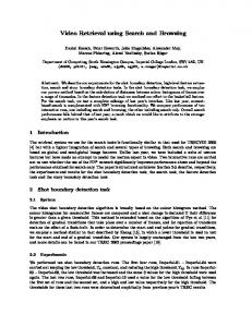
Two video sequences with NVS equal to 0.9. . . . . . . . . . . . . . . Two video sequences with IVS equal to 1/3. . . . . . . . . . . . . . . . The Voronoi diagram of a three-frame video. . . . . . . . . . . . . . . The shaded area denotes the similar Voronoi region between the two sequences. . . . . . . . . . . . . . . . . . . . . . . . . . . . . . . . . . Examples of sequences with identical IVS’s but very different VVS’s. . The unshaded region is the Voronoi gap for this pair of video sequences with IVS one. . . . . . . . . . . . . . . . . . . . . . . . . . . . . . . . The error probability for the hamming cube at different values of ² and distances k between the vectors in the video. . . . . . . . . . . . . . . Values of ranking function Q(·) for a three-vector video sequence. Lighter colors correspond to larger values. . . . . . . . . . . . . . . . . . . . . Quantization of the HSV color space. . . . . . . . . . . . . . . . . . . Comparisons between the basic (broken-line) and ranked (solid) ViSig methods for four different signature sizes: m = 2, 6, 10, 14. . . . . . . Precision and recall performance for ranked ViSig method at m = 2, 6, 10, 14. . . . . . . . . . . . . . . . . . . . . . . . . . . . . . . . . . Comparison between dc metric (broken) and dbc distance (solid). . . . Comparison between the Ranked ViSig method with m = 6 (solid) and k-medoid with 7 representative vectors (broken). . . . . . . . . . . . . Comparison between the symmetric and asymmetric VSSr with m = 6.
3.5 3.6 3.7 3.8 3.9 3.10 3.11 3.12 3.13 3.14 4.1
. . . .
. . . .
. . . .
. . . .
. . . .
. . . .
. . . .
. . . .
. . . .
. . . .
Distribution of the metric d(x, y) for 100,000 random pairs of signature vectors in the coordinates of maxi=1,2,...,100 |d(x, si ) − d(y, si )| and mini=1,2,...,100 [d(x, si ) + d(y, si )]. Different colors correspond to metric values at different ranges. . . . . . . . . . . . . . . . . . . . . . . . .
19 22 28 29 33 36 39 40 45 49 53 56 59 69 70 71 72 73
92
v 4.2
Pruning-versus-Accuracy plots for the “lower-bound”, the “product” and the proposed schemes. . . . . . . . . . . . . . . . . . . . . . . . . 4.3 Pruning-versus-accuracy plot for two dimension. . . . . . . . . . . . . 4.4 Pruning-versus-accuracy plot for four dimension. . . . . . . . . . . . 4.5 Pruning-versus-accuracy plot for eight dimension. . . . . . . . . . . . 4.6 Pruning and Accuracy versus pruning threshold for three independent sets of queries. . . . . . . . . . . . . . . . . . . . . . . . . . . . . . . 4.A The left figure shows the signature similarity search that uses the ranking of the query signature. The system on the right uses the rankings of the signatures in the database. Since the right system only needs to access the top-ranked signature vectors, less memory is required to store the database. . . . . . . . . . . . . . . . . . . . . . . . . . . . . 5.1 5.2
A threshold graph with three connected components. . . . . . . . . . . Precision versus recall for different clustering algorithms and simple thresholding. . . . . . . . . . . . . . . . . . . . . . . . . . . . . . . . . 5.3 Precision and Recall versus edge density threshold γ. . . . . . . . . . 5.4 Distribution of cluster sizes. . . . . . . . . . . . . . . . . . . . . . . . 5.A For both illustrations, we obtain a contradiction by replacing e of length d with a shorter edge (u, v) to obtain a better MST. . . . . . . . . . .
96 100 101 102 103
107 113 119 121 122 127
vi
List of Tables 2.1
Statistics of collected web video sequences . . . . . . . . . . . . . . . .
3.1
Comparison between using uniform random and corel image seed vectors. The second through fifth columns are the results of using uniform random seed vectors and the rest are the corel image seed vectors. Each row contains the results of a specific test video at IVS levels 0.8, 0.6, 0.4 and 0.2. The last two rows are the averages and standard deviations over all the test sequences. . . . . . . . . . . . . . . . . . . . . . . . . Comparison between VSSb and VSSr under different levels of perturbation. The table follows the same format as in Table 3.1. The perturbation levels ² tested are 0.2, 0.4, 0.8, 1.2 and 1.6. . . . . . . . . . . .
3.2
25
63
65
4.1
Speed comparisons among the sequential search, the proposed scheme, Fastmap, and Haar Wavelet. . . . . . . . . . . . . . . . . . . . . . . . 104
5.1
Statistics of the largest ten clusters in the database. . . . . . . . . . . 123
vii
Acknowledgements I am deeply indebted to my advisor and mentor, Professor Avideh Zakhor, for her guidance and inspiration throughout my graduate career at Berkeley. I am truly grateful for her dedication to the quality of my research, and her insightful prospectives on numerous technical issues. This work has also benefited from helpful discussions with several individuals. I would like to thank Prof. Lawrence A. Rowe for helping me to identify a number of key issues in my dissertation work, and always leaving his door open for discussions. I would also like to thank Professor Ray R. Larson for his helpful comments during my qualifying examination and dissertation talk. I am very grateful to both Professor Rowe and Professor Larson for reading earlier drafts of this dissertation. I would also like to thank Professor Alistair Sinclair for introducing me to many of the theoretical results in similarity search. In addition, I would like to express my gratitude to Rainer Lienhart from Intel Research Lab, and Frederic Dufaux from Compaq Cambridge Research Lab for providing the necessary video capturing routines and hyperlink datasets to begin my research. The financial support for my research work in last three years is greatly appreciated. They include funding from AFOSR Muri Grant FDF49620-99-1-0062, NSF grant CCR-9903368, California Digital Media Innovation (DiMI) program D97-03, and Hughes Research Lab. The companionship and support from students in the department are gratefully
viii acknowledged. In particular, many thanks to Thinh Nguyen, Daniel Tan, Vito Dai, Nelson Chang, Ralph Neff, John Koo, and Christian Frueh, for the insightful discussions on diverse research problems, for the tremendous help in both technical and personal matters, and for showing me that difficult problems can actually be solved in tennis court and soccer field. I am most grateful to my parents for instilling in me the importance of science and technology at a very young age, for encouraging me to pursue my own dream, and for reminding me the importance of doing my best even in the most difficult time. Finally, I would like to thank my wife Blanca for her love, her help and her support in my final stage of dissertation research and thesis writing. It was absolutely wonderful to have some one, late at night while I was stuck at a programming problem, bringing me a cup of hot coffee or a bowl of sweet grapes.
1
Chapter 1 Inroduction The amount of information on the world wide web has grown enormously since its creation in 1990. By June 2002, commercial search engines such as Google and Fast had indexed more than two billion web-pages. There is no central management on the web, so duplication of content is inevitable. There have been a number of research studies in recent years that investigated duplicated or highly-similar web-pages and web-sites [1, 2, 3, 4, 5]. The amount of redundancy on the web, as shown by these studies, is in fact quite high – one study has shown that about 46% of all the text documents on the web have at least one “near-duplicate,” that is a document which is identical except for low level details such as formatting, and 5% of them have between 10 and 100 replicas [2]. Overly-duplicated content wastes resources in storage and transmission bandwidth, and increases the effort required to mine information for both human and artificial agents.
2 Such a problem is more severe for web multimedia content, especially for web video sequences. Tens or even hundreds of very similar video clips are returned when sending popular video keywords such as “star wars” or “Clinton testimony” to commercial search engines. There are a number of factors contributing to such a high degree of multiplicity. Due to the stringent requirements in bandwidth and delay, web video sequences are often stored in multiple locations, formatted to various sizes and frame-rates, and compressed with different algorithms and bitrates to facilitate downloading and streaming. As multimedia authoring tools are now commonplace on personal computers, similar versions, in part or as a whole, of the same video can also be found on the web when users modify and combine original content with their own productions. Advances in automatic video analysis also enable users to easily create trailers or key-frame story-boards to summarize video sequences. All the aforementioned variations of the same video sequence share a large percentage of visually similar frames with each other. These are the types of similar video sequences we are interested in finding on the web. Identifying these similar content can be beneficial to content owners and web video applications such as the followings: • As users typically do not view items beyond the first result screen from a search engine [6], it is detrimental to have all “near-duplicate” entries cluttering the top retrievals. It is better to group together similar entries before presenting the retrieval results to users. Commercial search engines such as Google and Altavista have already applied techniques to cluster similar text documents
3 together before presenting them to users. • When a particular web video becomes unavailable or suffers from slow network transmission, users can opt for a better version among similar video content identified by the video search engine. • Similarity detection algorithms can also be used for content identification when conventional techniques such as watermarking are not applicable. For example, multimedia content brokers may use similarity detection to check for copyright violation as they have no right to insert watermarks into original material. In this dissertation, we explore the design and implemention of video similarity detection and search algorithms for large databases of video sequences such the web. There are three main challenges in building such a system: first, to design a robust and low-complexity video similarity measure; second, to support fast similarity search over potentially millions of video sequences, and third, to present the search results to users in an organized and intuitive manner. We propose, in this dissertation, a number of algorithms to tackle these problems, and demonstrate the efficiency and effectiveness of these algorithms on a large dataset of web video sequences. Before embarking on a detailed description of our system, we will first elaborate on these challenges and review existing solutions in the literature.
4
1.1
Video similarity measurement
As mentioned earlier, we are interested in defining a video similarity measure based on the percentage of visually similar frames or shots shared between two video sequences. This is analogous to finding the percentage of shared words or phrases between two text documents. This commonly-used document similarity measure is called a Tanimoto measure [1, 2]. While it is relatively straightforward to distinguish two different words,1 it is much harder to identify visually similar frames or shots due to the large number of possible variations. The typical approach is to identify each frame or shot by some of its attributes such as color, texture, shape, and motion, usually represented as a high-dimensional feature vector. Visual similarity between different frames can then be gauged by a metric function between the corresponding feature vectors. To compute our target video similarity measure, we thus need to identify feature vectors from two video sequences that are “close” to each other based on the computed metric values. There exist other video similarity measures in the literature and some of them are reviewed in this section. Nonetheless, no matter which measure is used, the major challenge is how to perform the measurement efficiently. As a video sequence can potentially have thousands of feature vectors representing different shots, computing a high-dimensional metric between them becomes a daunting task. On the other hand, for every new video added to the database or a query 1
Variants of the same word should be first converted to the root by a process known as word stemming [7, ch. 3]. Synonyms can also be identified as a unique lexical concept via the use of an electronic thesaurus [8].
5 video presented by a user, similarity measurements need to be performed with possibly millions of entries in the database. Thus, it is imperative to develop fast methods to compute similarity measurements for database applications. Finding visually similar content is the central theme in the area of Content-Based Information Retrieval (CBIR). In the past decade, numerous algorithms has been proposed to identify visual content similar in color, texture, shape, motion and many other attributes [9, 10, 11, 12, 13]. Much of the video similarity research has been focused on the problem of search for a particular short segment, such as a television commercial, within a long sequence [14, 15, 16, 17]. When extending the similarity measurement to full video, the first challenge is to define a single measurement to gauge the similarity between two video sequences. To this end, several proposals can be found in the literature: in [18, 19, 20], warping distance is used to measure the temporal edit differences between video sequences. Hausdorff distance is proposed in [21] to measure the maximal dissimilarity between shots. Template matching of shot change duration is used by Indyk et al. [22] to identify the overlap between video sequences. A common step shared by all the above schemes is to match similar feature vectors between two video sequences. This usually requires searching through part of or the entire video. The full computation of these measurements thus require the storage of the entire video, and time complexity that is at least linear in the length of the video. Applying such computations to find similar content within a database of millions of video sequences is too complex in practice.
6 On the other hand, computing the precise value of a similarity measurement is typically unnecessary. As feature vectors are idealistic models and do not entirely capture the process of how similarity is judged in the human visual system [23], many CBIR applications only require an approximation of the underlying similarity value. As such, it is unnecessary to maintain full fidelity of the feature vector representations, and approximation schemes can be used to alleviate high computational complexity. For example, in a video similarity search system, each video in the database can be summarized into a compact fixed-size representation that can be compared to test the similarity between the two video sequences. Two types of summarization techniques are used for similarity approximation: higher-order and first-order. Higher-order techniques summarize all feature vectors in a video as a statistical distribution. These techniques are useful in classification and semantic retrieval as they are highly adaptive and robust against small perturbation. Nonetheless, they typically assume a restricted form of density models such as Gaussian, or mixtures of Gaussian distributions, and require computationally intensive methods such as Expectation-Maximization for parameter estimation [24, 25, 26]. As a result, higher-order techniques may be impractical for matching the enormous amount of extremely diverse video content on the web. First-order techniques summarize a video by a small set of representative feature vectors. One approach is to compute the “optimal” representative vectors by minimizing the distance between the original video and its representation. If the metric is finite-dimensional Euclidean
7 and the distance is the sum of squared metric, the well-known k-means method can be used [27]. For general metric spaces, we can use the k-medoid method which identifies k feature vectors within the video to minimize the distance [28, 21]. Both of these algorithms are iterative with each iteration running at O(l) time for k-means, and O(l2 ) for k-medoids, where l represents the length of the video. To summarize long video sequences, such as feature-length movies or documentaries, these methods are clearly too complex to be used in large databases. To produce a compact summarization that is both easy to generate and capable of producing a reliable estimate of the underlying similarity, we propose a class of randomized techniques called the Video Signature (ViSig) method in Chapter 3. The ViSig method summarizes each video sequence in the database by selecting a number of its frames closest to a set of random vectors. Such a representation is called a video signature. An important result shown in Chapter 3 is that, regardless of how long the video sequences are, it is sufficient to use very small video signatures to identify those sequences that share a large fraction of similar frames. Our proposed ViSig method is also an example of first-order video summarization technique. Unlike the k-means or k-medoid methods, it is a single-pass O(l) algorithm. Thus, it takes far less computation to generate a summarization for a long video sequence. On the other hand, as demonstrated by the experimental results in Chapter 3, ViSig can produce retrieval results that are comparable to other techniques that are much more computationally intensive.
8
1.2
Fast similarity Search
An efficient algorithm to measure video similarity is only the first step towards building a similarity video search engine. When a user presents a query in the form of a video signature to the search engine, the search engine must identify all similar signatures in the database of possibly millions of entries. The naive approach of sequential search is too slow to handle large databases, and complex comparison functions. To guarantee a fast response time, it is imperative to develop fast similarity search algorithms. Faster-than-sequential solutions have been extensively studied by the database community. Elaborate data structures, collectively known as the Spatial Access Methods (SAM), have been proposed to facilitate similarity search [29, 9, 30]. Most of these methods, however, do not scale well to high dimensional metric spaces [31]. This problem is commonly known as the “curse of dimensionality”. One possible strategy to mitigate this problem is to design a transformation to map the original metric space to a low-dimensional space where a SAM structure can be efficiently applied. Such a transformation is called feature extraction mapping, and the approach of combining feature extraction with SAM is called GEneric Multimedia INdexIng (GEMINI) [9, ch. 7]. A good feature extraction mapping should be able to closely approximate distances in the high-dimensional space using the corresponding distances in the lowdimensional projected space. The most commonly used feature extraction mapping is Principal Component Analysis (PCA). PCA has been shown to be optimal in ap-
9 proximating Euclidean distance [32], and a myriad of techniques have been developed for generating PCA on large datasets [33]. If the underlying metric is not Euclidean, PCA is no longer optimal and more general schemes need to be used. Multidimensional Dimension Scaling (MDS) is the most general class of techniques for creating mappings that preserve a high-dimensional metric in a low-dimensional space [34]. Historically, MDS schemes have been developed for visualizing high-dimensional data on a computer screen. MDS solves a non-linear optimization problem by searching for the mapping that best approximates all the high-dimensional pairwise distances between data points. In most occasions, MDS is simply too complex to be used for similarity search. There are other techniques less computationally intensive techniques that are developed for metric spaces. One such technique is the Fastmap algorithm proposed by Faloutsos and Lin [35]. Fastmap is a heuristics algorithm that uses Euclidean distance to approximate a general metric. The time complexity of generating a fastmap mapping is linear with respect to the size of the database. In Section 4.3, we compare the search performance of fastmap with our proposed technique. Another class of techniques constructs feature extraction mappings based on distances between the high-dimensional vectors and a set of random vectors. These kinds of “random mappings” have been shown to possess certain favorable theoretical properties. [36] and [37] have shown that a specific form of the random mappings can achieve the best possible approximation of high-dimensional distances. Unfortunately, such mappings
10 are quite complex, and effectively require the computations of all pairwise distances. A more practical version has been proposed in [38] for approximating a metric used in protein sequencing. An even simpler version, called Triangle-Inequality Pruning (TIP), has been proposed by Berman and Shapiro for similarity search on image databases [39]. In Chapter 4, we propose a novel feature extraction mapping for metric-space data. This technique improves upon TIP by taking into account both the upper and lower bounds offered by the triangle-inequality. It also exploits the classical PCA technique in order to achieve any target dimension. As we will demonstrate in Chapter 4, our proposed scheme outperforms many other techniques in the literature in terms of the search performance on a large database of video signatures.
1.3
Similarity clustering
For a meaningful presentation of similarity search results, we investigate the use of clustering algorithms on a large database of video signatures. The goal is to group similar video sequences into non-overlapping clusters so a user is presented an uncluttered view of the results. A clustering structure provides an efficient organization of data which allows users to rapidly focus on relevant information. For example, clustering is extensively used in the areas of browsing and navigation [40, 41] as well as story segmentation of video clips [42, 43]. There are other benefits to applying clustering techniques to large databases. It has long been observed that clustering similar data items can improve the performance of a text-based information retrieval
11 system [44]. A number of recent studies have demonstrated that retrieval performance on multimedia information systems can also be improved via clustering [45, 21, 25]. Clustering experiments on web text documents show that the number of clusters with similar documents is likely to be very large [1]. It is difficult to apply many popular optimization-based clustering algorithms, such as the k-means method, to our problem as many of them need the precise number of clusters as input [46, ch. 14]. Another popular class of clustering algorithms, called the hierarchical algorithms, do not have such a requirement [46, ch. 13]. Hierarchical algorithms recursively create new clusters by either subdividing or merging existing ones. Different hierarchical algorithms use different criteria to decide which clusters to merge or divide. A common approach is based on the distances between centroids of the existing clusters. Nevertheless, in general metric spaces where distances are the only measurable quantities, there may not be a sensible way to compute the centroid of a cluster. In addition, as the ViSig method is a randomized algorithm, there are uncertainties associated with each signature. Centroids computed based on erroneous signature vectors certainly do not reflect the actual locations of the clusters. Rather than computing centroids, we can treat each data point as a vertex of a graph, and form edges between two data points if their distances are less than a certain threshold. The hierarchical clustering algorithm then considers the graphs formed at different thresholds, and identifies parts of the graphs as clusters based on their degree of connectivity. The simplest of such algorithms are the single-link and
12 complete-link algorithms [46]. The single-link algorithm identifies all the connected components in the graph as clusters, and the complete-link uses complete subgraphs. Both algorithms are viable candidates for clustering, but the results obtained by applying them to our data are dissatisfactory. The problem with the single-link algorithm is that its cluster definition is too lenient. As a result, a single-link algorithm produces some large clusters that contain totally irrelevant video clips. The cluster definition of the complete-link algorithm, in contrast, is too stringent – it dismisses true clusters in the presence of one single erroneous distance measurement. Ideally, a clustering algorithm should aim at identifying clusters between these two extremes of single-link and complete-link. In Chapter 5, we propose a new hierarchical clustering algorithm that allows the user to adjust the desirable level of connectivity for cluster identification. In the proposed algorithm, a connected component forms a cluster if its edge density exceeds a user-defined threshold. Not only does the proposed algorithm produce favorable retrieval results, it admits a simple implementation based on the classical Minimum Spanning Tree (MST) algorithm by Kruskal [47]. In [48], Zahn has used MST to separate data into different clusters if the MST branch connecting them is significantly longer than the nearby edges [48]. We extend this concept to consider the connectivity of the clusters. Recently, a number of graph-theoretical clustering algorithms based on network-flow algorithms have been proposed for visual grouping and gene expression clustering [49, 50]. Compared to MST, these techniques are far
13 more computationally intensive, and are thus difficult to scale to very large databases.
1.4
Organization
This dissertation is organized as follows: we first provide, in Appendix 1.A, a list of all the commonly-used acronyms and notations in this dissertation. Chapter 2 provides an overview of the design of a similarity video search engine. This design overview provides a functional description of how individual components proposed in this dissertation can be applied to a realistic design. This search engine can be accessed on the web at http://www-video.eecs.berkeley.edu/~cheungsc/cluster. The dataset of web video sequences, which we use throughout this dissertation, is also described in this chapter. Chapter 3 is devoted to video similarity measurement. Different video similarity models are discussed in this chapter, but the focus is on developing the ViSig method and its variations. We introduce the geometric interpretation of the ViSig method as an estimation of the intersecting volume between voronoi diagrams. This leads to the design of a number of heuristics that are essential to applying ViSig to real data. We present both experimental and simulation results to demonstrate the performance of ViSig. Chapter 4 deals with fast similarity search on large databases of video signatures. After a brief review of a generic similarity search procedure, we focus on designing the feature extraction mapping on high-dimensional video signatures to low-dimensional
14 index vectors. The two main components of this mapping, namely the projection vector mapping and the PCA, are described in detail. Finally, we compare the search performance on randomly queries between the proposed technique and other stateof-the-art methods. Chapter 5 discusses how clustering can be applied to improve retrieval performance. We first introduce the graphical representation of a database of video signatures, and define similar clusters as highly connected regions inside the graph. We then explain how these similar clusters can be identified by using a simple modification of Kruskal’s minimum spanning tree algorithm. Experimental results are then presented comparing the proposed algorithm with simple thresholding, single-link and complete-link hierarchical clustering algorithms. Finally, we apply our algorithm to a large database of web video sequences, and statistically analyze the resulting clustering structure. Chapter 6 presents a summary of the results in this dissertation along with suggestions for future work. Portions of Chapter 3 have appeared in [51, 52, 53, 54, 55], while parts of Chapters 4 and 5 have been presented in [56, 57].
15
1.A
Appendix: Acronyms and Notations
Acronyms NVS IVS VVS ViSig VSSb PDF VSSr HSV GEMINI CC MST
Na¨ıve Video Similarity Ideal Video Similarity Voronoi Video Similarity Video Signature Basic ViSig Similarity Probability Density Function Ranked ViSig Similarity Hue-Saturation-Value color space Generic Multimedia Indexing Connected Component Minimum Spanning Tree
Notations (F, d(·, ·)) Feature vector space F with metric d(·, ·) x, y Video frames, represented as feature vectors X, Y Video sequences, represented as sets of feature vectors ² Frame Similarity Threshold 1X Indicator function |X| Cardinality of set X nvs(X, Y ; ²) NVS between X and Y [X]² Collection of clusters in X [X ∪ Y ]² Clustered union between X and Y ivs(X, Y ; ²) IVS between X and Y V (X) Voronoi Diagram of video X VX (x) Voronoi Cell of x ∈ X VX (C) Voronoi Cell of a cluster C ∈ [X]²
16 R(X, Y ; ²) Vol(A) Prob(A) vvs(X, Y ; ²) XS gX (s), xs vssb (XS , YS ; ², m) m f (u; X ∪ Y )
Similar Voronoi Region Volume of a region A Probability of event A VVS between X and Y Signature of X with respect to the SV set S Signature vector of X with respect to s VSSb between XS and YS Number of signature vectors in a signature PDF that assigns equal probability to the Voronoi Cell of each cluster in [X ∪ Y ]² G(X, Y ; ²) Voronoi gap between X and Y Q(gX (s)) Ranking function for the signature vector gX (s) vssr (XS , YS ; ², m) VSSr between XS and YS m0 Number of top-ranked signature vectors used in computing VSSr vss dr (XS , YS ; ², m) Asymmetric VSSr between XS and YS using the ranking of XS q q b dc (xi , yi ), dc (xi , yi ) l1 and modified l1 color histogram distances dc (x, y), dbc (x, y) Quadrant color histogram distances based on dqc (·, ·) and dbqc (·, ·) ρ Dominant color threshold used in dbqc (·, ·) rel(X) The set of video sequences that are subjectively similar to video X as defined in the ground-truth set ret(X, ²) The set of video sequences that are declared to be similar to X by the ViSig method at ² level Recall(²) The recall in retrieving the ground-truth by the ViSig method at ² level Precision(²) The precision in retrieving the ground-truth by the ViSig method at ² level A(x; ²) The result set of similarity search on feature vector x AS (XS ; ²) The result set of similarity on signature XS 0 ² Pruning threshold 0 C(x; ² ) The GEMINI candidate set for feature vector x C(XS ; ²0 ) The GEMINI candidate set for signatures XS A0 (x; ², ²0 ) The GEMINI result set for feature vector x A0 (XS ; ², ²0 ) The GEMINI result set for signature XS 0 0 (F , d (·, ·)) Range space and Range metric T (x) Feature extraction mapping of feature vector x P(x) Projection vector mapping of feature vector x dsig (·, ·) Signature distance
17 V (G) E(G) P (V, ρ) Γ(G) γ
Vertex set of a graph G Edge set of a graph G Threshold graph on vertex set V and distance threshold ρ Edge density of graph G Edge density threshold
18
Chapter 2 A similarity video search engine This chapter describes a similarity video search engine that utilizes all our proposed algorithms, as well as the dataset behind this engine and other experiments presented throughout the dissertation. The functional description of the search engine can be found in Section 2.1. A prototype of this engine can be accessed at http://www-video.eecs.berkeley.edu/~cheungsc/cluster. Section 2.2 describes the web video dataset behind this search engine and the data collection process. We also derive a ground-truth set from this dataset to measure the retrieval performance of various algorithms. The construction of the ground-truth set is described in Section 2.3.
19
2.1
System description
The architecture of our proposed search engine is shown in Figure 2.1. The Uniform Resource Locator or URL database contains a large number of URL addresses of video hyperlinks, which are acquired by traversing the web with a web crawler. The web video capturer reads the URL addresses from the URL database, downloads the corresponding video clip, and identifies relevant meta-data terms. Meta-data terms are textual information about the video clip. They consist of terms extracted from the URL address of the video hyperlink, the description of the hyperlink, the title and address of the web-page, and auxiliary information such as the creator’s name and the copyright notice embedded in the clip. The meta-data terms are stored in the cluster & meta-data database, while the video-data is sent to the signature & index generation process.
Signature & Index Generation Video Data
Web Web
Indices Signatures
Index Database Signature Database
Similarity Search
Signature Clustering
Video query Results
Keyword Search
Keyword query Results
Cluster Definition
Web Video Capturer Meta Data
Cluster & Meta-Data Database
URL database
Figure 2.1: Schematic of the video search engine.
During the signature & index generation process, a signature and an index are
20 generated for each input video clip. A signature is a compact representation of a video clip, while an index is an even smaller entity that is used to facilitate similarity search on signatures. Details on how indices are used to facilitate fast similarity search on signatures are described in Chapter 4. The video search engine uses similarity search in two different modes. First, it allows a user to search for video content in the search engine database that are potentially similar to the input query video clip. To do this, a user needs to first download software to produce a signature for his/her video clip. The signature is then sent to the search engine where a similarity search is performed. Thumbnail images and hyperlink information for all signatures within a small distance threshold of the query are then presented to the user. Similarity search is also used by the signature clustering process in our search engine. Based on the similarity search results of all the signatures, the signature clustering process identifies clusters of similar video sequences in the database. These similarity clusters can be used in many different ways: First, we show in Chapter 5 that it is possible to improve retrieval performance by returning similar clusters, rather than individual video, that are close to the input query. Second, we can use the resulting clusters to expand the results of keyword search, which is another function supported by our search engine. After the signature clustering process, membership information of all the clusters is stored in the cluster & meta-data database. For each meta-data term k in the database, we identify those clusters with at least one video clip that has k in its meta-data record. All these clusters will be returned if k is a
21 part of the user’s keyword search. This approach expands the simple paradigm of keyword search to include those visually similar video clips that may not have any meta-data term that matches the query keyword. To illustrate this concept via an example, consider querying our search engine with the keyword “telephone.” Figure 2.2 shows a screen-shot of the search results. Thumbnail images are used to represent returned clusters, which are ranked by the number of video clips in them. The detailed listing of all video clips is shown by clicking on the thumbnail image. As shown in the figure, 48 video clips relevant to the keyword “telephone” are retrieved, despite the fact that only eight clips actually have the term “telephone” in their meta-data records. These 48 video clips are organized into seven clusters of visually similar video sequences. The cluster organization provides the user a concise summary of all the visually distinctive video sequences among the search results.
2.2
Web video acquisition
In order to demonstrate the applicability of our algorithms, it is important to base our results on a representative collection of video sequences on the web. Most experimental results presented in this dissertation are based on a collection of 46,331 video sequences, crawled from the web between June and December of 1999. This section briefly describes the approach used to acquire these sequences as well as the nature of the web video sequences in our collection. A common approach to collect data from the web is to use a web crawler. A web
22 crawler is a program that automatically traverses the web’s hyperlink structure and retrieves desired information. As video sequences are sparsely distributed over the web, a web crawler requires substantial amount of time and resources to collect a representative data-set. Our approach to building a video collection is to send a large set of queries to the AltaVista video search engine to obtain URL addresses of web
Figure 2.2: Search results of keyword “telephone”.
23 video sequences. Similar methods have been used to estimate the size of the web [58]. To avoid bias towards particular types of content, our query word set consists of about 300,000 words obtained from a general search engine [59], an Internet videoon-demand site [60] and a speech recognizer vocabulary [61]. All query requests are carefully controlled so as not to overburden the search engine. Over the entire month of June 1999, about 62,000 URL addresses pointing to video content were obtained. This data-set constitutes roughly 15% of all the non-broadcast video clips on the web at that time, according to the figure estimated by Compaq Cambridge Research Laboratory in November 1998 [62]. The second step is to follow the resulting URLs and download the actual video sequences. Among all the video URLs, the most popular formats are RealVideo, Quicktime, MPEG-1, and AVI. Except for MPEG-1 which is an open standard [63], the remaining formats are proprietary. This has a significant impact on the download time since no fast bit-stream level processing can be applied, and the video sequences can only be captured after full decoding. In other words, the capture time is limited by the decoding speed or even real-time display in certain formats. RealVideo streaming format [64] presents an additional level of challenge since its display quality depends on the network conditions during the download. Depending on the settings of the content server, heavy packet losses on the network may cause delay, frame drops or corrupted frames. We developed capture software that takes the delay due to packet losses into account but fails to detect frame drops or corrupted frames. As
24 a result, the quality of the captured video sequences may vary significantly even for the same video downloaded from two different locations. In order to reduce storage requirements, all video sequences are re-sampled at three frames per second. For each sequence, almost identical neighboring frames with peak signal to noise ratio larger than 50 dB are removed, and the remaining frames are compressed using motionJPEG. After eliminating synonymous1 and expired URL entries, we capture 46,331 video clips with total duration of approximately 1800 hours. The total disk space required for the motion-JPEG video sequences exceeds 100 Gigabytes. The total capture time was approximately 30 days using four Intel Pentium-based personal computers. In other words, on average, it takes 1.6 hours to capture 1 hour of video. The bottleneck in capturing is primarily due to the buffering delay in recording streaming RealVideo. The statistics of the four most abundant types of collected video sequences are shown in Table 2.1. Except RealVideo video sequences, most of the other sequences are less than one minute long.
2.3
Ground-truth construction
A ground-truth set is commonly used as an experimental tool to measure how well an automatic retrieval algorithm can match human judgment [44, 98]. A general 1
Synonymous URLs are detected using the following heuristics [65] : (i) removing the port 80 designation (the default), (ii) removing the first segment of the domain name for URLs with a directory depth greater than one (to account for machine aliases), and (iii) unescaping any “escaped” characters.
25 Video Type MPEG QuickTime RealVideo AVI
% over all clips 31 30 22 16
Duration (mean ± std-dev in minutes) 0.26 ± 0.7 0.51 ± 0.6 9.57 ± 18.5 0.16 ± 0.3
Table 2.1: Statistics of collected web video sequences
ground-truth set consists of multiple clusters of data items from a large dataset. Each cluster of the ground-truth set contains all the items in the dataset that are considered to be relevant to a particular concept by a group of human subjects. By presenting each data item in the ground-truth set as a query to an automatic retrieval system, we can measure how well the system can approach human judgment. In our particular application, the ground-truth set contains clusters of highly similar video sequences from the web video dataset. Ideally, each group in the groundtruth set should capture all of the similar versions of the same video content in the entire dataset. Rather than manually examining the entire set of more than 1800 hours of video, we adopt a best-effort approach to obtain such a ground-truth. This approach is similar to the pooling method commonly used in text retrieval systems [44]. The basic idea of pooling is to first send the same queries to different automatic retrieval systems, other than the one being tested. Then, the top-ranked results from these systems are pooled together and examined by human experts to identify the truly relevant ones. The goal of pooling is to reduce human effort by using automatic systems to eliminate a large number of irrelevant results.
26 For our system, the first step is to use meta-data terms to identify the initial ground-truth clusters. As described in Section 2.2, meta-data terms are extracted from the URL address and other textual information of each video. All video sequences in the dataset containing at least one of the top 1000 most frequently used meta-data terms are manually examined and grouped into clusters of similar video. Clusters which are significantly larger than others are removed to prevent bias. We obtained 107 clusters which form the initial ground-truth clusters. This method, however, may not be able to identify all the video clips in the dataset that are similar to those already in the ground-truth clusters. We further examined those video sequences in the dataset that share at least one meta-data term with the ground-truth video, and add any similar video to the corresponding clusters. In addition to meta-data, we apply visual similarity scheme to enlarge the groundtruth as well. In particular, we identify video sequences in the dataset with color distribution similar to those already in the ground-truth. It has been shown that color is one of the most important low-level visual cue in identifying similar visual content [70]. We briefly describe here how we expand the ground-truth with color similarity, but defer all the technical details of similarity measurement until Section 3.7. We first convert every frame of a video into a color histogram feature vector. Then, each video clip in the dataset and the ground-truth set is summarized as a k-medoid of seven feature vectors. As mentioned in Chapter 1, k-medoid is a summarization technique that minimizes the distance between the original video and
27 its summarization [28, 21]. For each k-medoid X in the ground-truth, we identify 100 k-medoids in the dataset that are closest to X in terms of the minimum distance between all the vectors in their corresponding k-medoid representations. These 100 video clips are again manually examined to identify those visually similar to X. As a result, we obtain a ground-truth set consisting of 443 video sequences in 107 clusters. These ground-truth clusters and their sizes are shown in Figures 2.3 and 2.4. Each cluster is represented by a video frame randomly selected from one of the sequences within the cluster. The cluster size ranges from 2 to 20, with average size equal to 4.1. For all our retrieval experiments, these ground-truth clusters serve as the basis for comparison against those similar video sequences identified by the automatic retrieval algorithms.
28
Figure 2.3: Ground-truth clusters and their sizes (part 1 of 2).
29
Figure 2.4: Ground-truth clusters and their sizes (part 2 of 2).
30
Chapter 3 Measuring video similarity This chapter defines the video similarity models used in this dissertation, and describes how they can be efficiently estimated by the ViSig method. We assume that individual frames in a video sequence are represented by high-dimensional feature vectors from a metric space (F, d(·, ·))1 . In order to be robust against editing changes in the temporal domain, we define a video sequence X as a finite set of feature vectors and ignore any temporal ordering. For the remainder of this chapter, we make no distinction between a video frame and its corresponding feature vector. The metric d(x, y) measures the visual dissimilarity between vectors x and y. We assume that vectors x and y are visually similar to each other if and only if d(x, y) ≤ ² for an ² > 0 independent of x and y. We call ² the Frame Similarity Threshold. This chapter is organized as follows. Section 3.1 defines our target measure, called 1
For all x, y in F , the function d(x, y) is a metric if a) d(x, y) ≥ 0; b) d(x, y) = 0 ⇔ x = y; c) d(x, y) = d(y, x); d) d(x, y) ≤ d(x, z) + d(z, y), for all z ∈ F .
31 the Ideal Video Similarity (IVS), used in this chapter to gauge the visual similarity between two video sequences. As we explain in the section, this similarity measure is complex to compute exactly, and requires a significant number of vectors to represent each video. To reduce the computational complexity and the representation size, we propose an alternative form of video similarity called the Voronoi Video Similarity (VVS) in Section 3.2. This particular form of similarity leads directly to an efficient technique for representation and estimation called the ViSig method, described in detail in Section 3.3. Sections 3.4 through 3.6 analyze the scenarios where IVS cannot be reliably estimated by our proposed algorithm, and propose a number of heuristics to rectify the problems. Experimental results are presented in Section 3.7. We summarize this chapter in Section 3.8. The proofs to all propositions in this chapter can be found in Appendix 3.A.
3.1
Ideal video similarity
As mentioned in Chapter 1, we are interested in using a video similarity measure that is based on the percentage of visually similar frames between two sequences. A naive way to compute such a measure is to first find the total number of frames from each video sequence that have at least one visually similar frame in the other sequence. Then, compute the ratio of this number with the overall total number of frames as the final similarity value. We call this measure the Na¨ıve Video Similarity (NVS):
32 Definition 3.1.1 Na¨ıve Video Similarity Let X and Y be two video sequences. The number of vectors in video X that have at least one similar vector in Y can be computed by
P
x∈X
1{y∈Y : d(x,y)≤²} , where 1A is
the indicator function with 1A = 1 if A is not empty, and zero otherwise. The Na¨ıve Video Similarity between X and Y , nvs(X, Y ; ²), can thus be defined as follows: P P ∆ x∈X 1{y∈Y : d(x,y)≤²} + y∈Y 1{x∈X: d(y,x)≤²} nvs(X, Y ; ²) = , (3.1) |X| + |Y | where | · | denotes the cardinality of a set, or in our case the number of vectors in a given video. If every vector in video X has a similar vector in Y and vice versa, nvs(X, Y ; ²) = 1. If X and Y share no similar vectors at all, nvs(X, Y ; ²) = 0. Unfortunately, NVS does not always reflect our intuition of video similarity. Most real-life video sequences can be temporally separated into video shots, within which frames are visually similar. Among all possible versions of the same video, the number of frames in the same shot can be quite different. For instance, different coding schemes modify the frame rates for different playback capabilities, and video summarization algorithms use a single keyframe to represent an entire shot. As NVS is based solely on frame counts, its value is highly sensitive to these kinds of manipulations. To illustrate this problem with a pathological example, consider the two sequences shown in Figure 3.1. We represent the feature vector space as a 2-D square. Crosses and dots in the figure signify frames from two different video sequences X and Y respectively. X has two frames that are very far apart, while all the frames in Y are
33 clustered around one of the frames in X. This may happen, for example, when X is a key-frame sequence of a video with two distinct shots, and Y retains an entire shot of this video. Assume all eight frames in Y are within ² of that particular frame in X. Even though it is intuitive to say that the two sequences have 50% overlap, the measured NVS between X and Y is 90%. It is possible to rectify the problem by using shots as the fundamental unit for similarity measurement. Since we model a video as a set and ignore all temporal ordering, we instead group all visually similar vectors in a video together into non-intersecting units called clusters.
Figure 3.1: Two video sequences with NVS equal to 0.9.
A cluster should ideally contain only similar vectors, and no other vectors similar to the vectors in a cluster should be found in the rest of the video. Mathematically, we can express these two properties as follows: for all pairs of vectors xi and xj in
34 X, d(xi , xj ) ≤ ² if and only if xi and xj belong to the same cluster. Unfortunately, such a clustering structure may not exist for an arbitrary video X. Specifically, if d(xi , xj ) ≤ ² and d(xj , xk ) ≤ ², there is no guarantee that d(xi , xk ) ≤ ². If d(xi , xk ) > ², there is no consistent way to group all the three vectors into clusters. In order to have a general framework for video similarity, we adopt a relatively relaxed clustering structure by only requiring the forward condition, i.e. d(x i , xj ) ≤ ² implies that xi and xj are in the same cluster. A cluster is simply one of the connected components [66, appendix B] of a graph in which each node represents a vector in the video, and every pair of vectors within ² of each other is connected by an edge. We denote the collection of all clusters in video X as [X]² . It is possible for such a definition to produce chain-like clusters where one end of a cluster is very far from the other end. Nonetheless, given an appropriate feature vector and a reasonably small ², most clusters found in real video sequences are compact, i.e. all vectors in a cluster are similar to each other. We call a cluster ²-compact if all its vectors are within ² from each other. The clustering structure of a video can be computed by a simple hierarchical clustering algorithm called the single-link algorithm [67]. To define a similarity measure based on the visually similar portion shared between two video sequences X and Y , we consider the clustered union [X ∪Y ]² . If a cluster in [X ∪ Y ]² contains vectors from both sequences, these vectors are likely to be visually similar to each other. Thus, we call such a cluster a Similar Cluster and consider it as part of the visually similar portion. The ratio between the number of similar clusters
35 and the total number of clusters in [X ∪ Y ]² forms a reasonable similarity measure between X and Y . We call this measure the Ideal Video Similarity (IVS): Definition 3.1.2 Ideal Video Similarity, IVS Let X and Y be two video sequences. For each cluster C in [X ∪ Y ]² , C contains vectors from both X and Y if and only if 1C∩X · 1C∩Y = 1. Thus, we can define the IVS between X and Y , ivs(X, Y ; ²), as follows: ∆
ivs(X, Y ; ²) =
P
C∈[X∪Y ]²
1C∩X · 1C∩Y
|[X ∪ Y ]² |
(3.2)
The main theme of this chapter is to develop efficient algorithms to estimate the IVS between a pair of video sequences. A simple pictorial example, shown in Figure 3.2, demonstrates the use of IVS. Vectors closer than ² are connected by dotted lines. There are altogether three clusters in the clustered union, and only one cluster has vectors from both sequences. The IVS measure is thus 1/3. It is complex to precisely compute IVS. The clustering used in IVS depends on the distances between vectors from the two sequences. This implies that for two video sequences with l vectors each, one needs to first compute the distance between l2 pairs of vectors before running the clustering algorithm and computing the IVS. In addition, the computation requires the entire video to be stored. The complex computation and large storage requirements are clearly undesirable for large database applications. As the exact similarity value is often not required in many applications,
36
Figure 3.2: Two video sequences with IVS equal to 1/3.
sampling techniques can be used to estimate the true IVS. Consider the following simple sampling scheme: let each video sequence in the database be represented by m randomly selected vectors. We estimate the IVS between two sequences by counting the number of similar pairs of vectors Wm between their respective sets of sampled vectors. As long as the desired level of precision is satisfied, m should be chosen as small as possible to achieve low complexity. Nonetheless, even in the case when the IVS is as high as one, we show in the following proposition that we need a large m to find even one pair of similar vectors among the sampled vectors. Proposition 3.1.1 Let X and Y be two video sequences with l vectors each. Assume for every vector x in X, Y has exactly one vector y similar to it, i.e. d(x, y) ≤ ². We also assume the same for every vector in Y . Clearly, ivs(X, Y ; ²) = 1. The expectation
37 of the number of similar vector pairs Wm found between m randomly selected vectors from X and from Y is given below: E(Wm ) =
m2 . l
(3.3)
Despite the fact that the IVS between the video sequences is one, Equation (3.3) shows that we need, on average, m =
√
l sample vectors from each video to find
just one similar pair. Furthermore, comparing two sets of
√
l vectors requires l high-
dimensional metric computations. A better random sampling scheme should use a fixed-size record to represent each video, and require far fewer vectors to identify highly similar video sequences. Our proposed ViSig method is precisely such a scheme and is the topic of the following section.
3.2
Voronoi video similarity
As described in the previous section, the simple sampling scheme requires a large number of vectors sampled from each video to estimate IVS. The problem lies in the fact that since we sample vectors from two video sequences independently, the probability that we simultaneously sample a pair of similar vectors from them is rather small. Rather than independent sampling, the ViSig method introduces dependence by selecting vectors in each video that are similar to a set of predefined random feature vectors common to all video sequences. As a result, the ViSig method requires far
38 fewer sampled vectors to find a pair of similar vectors from two video sequences. The number of pairs of similar vectors found by the ViSig method depends strongly on the IVS, but does not have a one-to-one relationship with it. We call the form of similarity estimated by the ViSig method the Voronoi Video Similarity (VVS). The term “Voronoi” in VVS is borrowed from a geometrical concept called the Voronoi Diagram. Given a video X = {xt : t = 1, . . . , l}, the Voronoi Diagram V (X) of X is a partition of the feature space F into l Voronoi Cells VX (xt ). By definition, the Voronoi cell VX (xt ) contains all the vectors in F closer to xt ∈ X than to any ∆
other vectors in X, i.e. VX (xt ) = {s ∈ F : gX (s) = xt and xt ∈ X}, where gX (s) denotes the vector in X closest2 to s. A simple Voronoi diagram of a video is shown in Figure 3.3. We can extend the idea of the Voronoi diagram to video clusters by merging Voronoi cells of all the vectors belonging to the same cluster. In other words, ∆
for C ∈ [X]² , VX (C) =
S
x∈C
VX (x).
Given two video sequences X and Y and their corresponding Voronoi diagrams, we define the Similar Voronoi Region R(X, Y ; ²) as the union of all the intersection between the Voronoi cells of those x ∈ X and y ∈ Y where d(x, y) ≤ ²: ∆
R(X, Y ; ²) =
[
d(x,y)≤² 2
VX (x) ∩ VY (y).
(3.4)
If there are multiple x’s in X that are equidistant to s, we choose gX (s) to be the one closest to a predefined vector in the feature space such as the origin. If there are still multiple candidates, more predefined vectors can be used until a unique gX (s) is obtained. Such an assignment strategy ensures that gX (s) depends only on X and s but not some arbitrary random choices. This is important to the ViSig method which uses gX (s) as part of a summary of X with respect to a randomly selected s. Since gX (s) depends only on X and s, sequences identical to X produce the same summary vector with respect to s.
39
Figure 3.3: The Voronoi diagram of a three-frame video.
It is easy to see that if x and y are close to each other, their corresponding Voronoi cells are very likely to intersect in the neighborhood of x and y. The larger number of vectors from X and from Y that are close to each other, the larger the resulting R(X, Y ; ²) becomes. A simple pictorial example of two video sequences with their Voronoi diagrams is shown in Figure 3.4: dots and crosses represent the vectors of the two sequences; the solid and broken lines are the boundary between the two Voronoi cells of the two sequences represented by dots and crosses respectively. The shaded region shows the similar Voronoi region between these two sequences. Similar Voronoi region is the target region whose volume defines VVS. Before providing a definition of VVS, we need to first clarify what we mean by the volume of a region in the feature space.
40
Figure 3.4: The shaded area denotes the similar Voronoi region between the two sequences.
We define the volume function Vol : Ω → R to be the Lebesgue measure over the set, Ω, of all the measurable subsets in the feature space F [68]. For example, if F is the real line and the subset is an interval, the volume function of the subset is just the length of the interval. We assume all the Voronoi cells considered in our examples to be measurable. We further assume that F is compact in the sense that Vol(F ) is finite. Because we are going to normalize all volume measurements by Vol(F ), we assume that Vol(F ) = 1. To compute the volume of the similar Voronoi region R(X, Y ; ²) between two video sequences X and Y , we first notice that individual terms inside the union in Equation (3.4) are disjoint from each other. By the basic properties of Lebesgue measure, we have Vol(R(X, Y ; ²)) = Vol(
[
d(x,y)≤²
VX (x) ∩ VY (y)) =
X
d(x,y)≤²
Vol(VX (x) ∩ VY (y)).
41 Thus, we define the VVS between two video sequences X and Y as follows: ∆
vvs(X, Y ; ²) =
X
d(x,y)≤²
Vol(VX (x) ∩ VY (y))
(3.5)
The VVS of the two sequences shown in Figure 3.4 is the area of the shaded region, which is about 1/3 of the area of the entire feature space. Notice that for this example, the IVS is also 1/3. VVS and IVS are close to each other because the Voronoi cell for each cluster in the cluster union has roughly the same volume (area). In general, when the clusters are not uniformly distributed over the feature space, there can be a large variation among the volumes of the corresponding Voronoi cells. Consequently, VVS can be quite different from IVS. Before explaining how we can reconcile these two similarity measures, we first introduce the core algorithm in this chapter, the Basic ViSig method, as a randomized technique to estimate VVS.
3.3
Video signature method
It is straightforward to estimate vvs(X, Y ; ²) by random sampling. First, generate a set S of m independent uniformly distributed random vectors s1 , . . . , sm , which we call Seed Vectors. By uniform distribution, we mean for every measurable subset A in F , the probability of generating a vector from A is Vol(A). Second, for each seed vector s ∈ S, determine if s is inside R(X, Y ; ²). By definition, s is inside R(X, Y ; ²) if and only if s belongs to some Voronoi cells VX (x) and VY (y) with d(x, y) ≤ ². Since s must be inside the Voronoi cell of the vector closest to s in the entire video
42 sequence, i.e. gX (s) in X and gY (s) in Y , an equivalent condition for s ∈ R(X, Y ; ²) is d(gX (s), gY (s)) ≤ ². Since we only need gX (s) and gY (s) to determine if each seed ∆
vector s belongs to R(X, Y ; ²), we can summarize video X by the m-tuple XS = (gX (s1 ), . . . , gX (sm )) and Y by YS . We call XS and YS the Video Signature (ViSig), or simply signature, with respect to S of video sequences X and Y respectively. In the final step, we compute the percentage of signature vector pairs gX (s) and gY (s) with distances less than or equal to ² to obtain: m X
1{d(gX (si ),gY (si ))≤²}
∆ i=1
vssb (XS , YS ; ², m) =
m
.
(3.6)
We call vssb (XS , YS ; ², m) the Basic ViSig Similarity (VSSb ) between signatures XS and YS . As every seed vector s ∈ S in the above algorithm is chosen to be uniformly distributed, the probability of s being inside R(X, Y ; ²) is simply the VVS between X and Y . Thus, vssb (XS , YS ; ², m) forms an unbiased estimator of the VVS between X and Y . We refer to this approach of generating a signature and computing VSSb the Basic ViSig method. To apply the Basic ViSig method to a large number of video sequences, we must use the same seed vector set S to generate all the signatures in order to compute VSSb between an arbitrary pair of video sequences. The number of seed vectors in S, m, is an important parameter. On one hand, m represents the number of samples used to estimate the underlying VVS and thus, a large m produces a more accurate estimation. On the other hand, the complexity of the Basic ViSig method depends on m. If a video has l vectors, it takes l metric
43 computations to generate a single signature vector. The number of metric computations required to compute the entire signature is thus m · l. Also, computing the VSS b between two signatures requires m metric computations. It is, therefore, important to determine an appropriate value of m that can satisfy both the desired estimation fidelity and the computational resources of a particular application. The following proposition provides an analytical bound on m in terms of the maximum error in estimating the VVS between any pair of video sequences in a database: Proposition 3.3.1 Assume we are given a database Λ with n video sequences and a set S of m random seed vectors. Define the error probability Perr (m) to be the probability that any pair of video sequences in Λ has their m-vector VSSb different from the true VVS value by more than a given γ ∈ (0, 1], i.e. ∆
Perr (m) = Prob
³ [
X,Y ∈Λ
{|vvs(X, Y ; ²) − vssb (XS , YS ; ², m)| > γ}
´
(3.7)
A sufficient condition to achieve Perr (m) ≤ δ for a given δ ∈ (0, 1] is as follows: m ≥
2 ln n − ln δ 2γ 2
(3.8)
It should be noted that the bound (3.8) in Proposition 3.3.1 only provides a sufficient condition and does not necessarily represent the tightest bound possible. Nonetheless, we can use this bound to understand the dependencies of m on various factors. First, unlike the random sampling described in Section 3.1, m does not
44 depend on the length of individual video sequences. This implies that it takes fewer vectors for the ViSig method to estimate the similarity between long video sequences than random vector sampling. Second, we notice that the bound on m increases with the natural logarithm of n, the size of the database. The signature size depends on n because it has to be large enough to simultaneously minimize the error of all possible pairs of comparisons, which is a function of n. Fortunately, the slow-growing logarithm makes the signature size rather insensitive to the database size, making it suitable for very large databases. The contribution of the term ln δ is also quite insignificant. Comparatively, m is most sensitive to the choice of γ. A small γ means an accurate approximation of the similarity, but usually at the expense of a large number of sample vectors m to represent each video. The choice of γ should depend on the particular application at hand.
3.4
Seed vector generation
We have shown in the previous section that the VVS between two video sequences can be efficiently estimated by the Basic ViSig method. Unfortunately, the estimated VVS does not necessarily reflect the target measure of IVS as defined in Equation (3.2). For example, consider the two pairs of sequences in Figures 3.5(a) and (b). Dots and crosses are vectors from the two sequences, whose Voronoi diagrams are indicated by solid and broken lines respectively. The IVS’s in both cases are 1/3. Nonetheless, the VVS in Figure 3.5(a) is much smaller than 1/3, while that of Figure
45 3.5(b) is much larger. Intuitively, as mentioned in Section 3.2, IVS and VVS are the same if clusters in the clustered union are uniformly distributed in the feature space. In the above examples, all the clusters are clumped in one small area of the feature space, making one Voronoi cell significantly larger than the other. If the similar cluster happens to reside in the smaller Voronoi cells, as in the case of Figure 3.5(a), the VVS is smaller than the IVS. On the other hand, if the similar cluster is in the larger Voronoi cell, the VVS becomes larger. This discrepancy between IVS and VVS implies that VSSb , which is an unbiased estimator of VVS, can only be used as an estimator of IVS when IVS and VVS is close. Our goal in this section and the next is to modify the Basic ViSig method so that we can still use this method to estimate IVS even in the case when VVS and IVS are different.
(a)
(b)
Figure 3.5: Examples of sequences with identical IVS’s but very different VVS’s.
46 As the Basic ViSig method estimates IVS based on uniformly-distributed seed vectors, the variation in the sizes of Voronoi cells affects the accuracy of the estimation. One possible method to amend the Basic ViSig method is to generate seed vectors based on a probability distribution such that the probability of a seed vector being in a Voronoi cell is independent of the size of the cell. Specifically, for two video sequences X and Y , we can define the Probability Density Function (PDF) based on the distribution of Voronoi cells in [X ∪Y ]² at an arbitrary feature vector u as follows: ∆
f (u; X ∪ Y ) =
1 1 · |[X ∪ Y ]² | Vol(VX∪Y (C))
(3.9)
where C is the cluster in [X ∪ Y ]² with u ∈ VX∪Y (C). f (u; X ∪ Y ) is constant within the Voronoi cell of each cluster, with the value inversely proportional to the volume of that cell. Under this PDF, the probability of a random vector u inside the Voronoi cell VX (C) for an arbitrary cluster C ∈ [X ∪ Y ]² is given by
R
VX (C)
f (u; X ∪ Y ) du =
1/|[X ∪ Y ]² |. This probability does not depend on C, and thus, it is equally likely for u to be inside the Voronoi cell of any cluster in [X ∪ Y ]² . Recall that if we use uniform distribution to generate random seed vectors, VSS b forms an unbiased estimate of the VVS defined in Equation (3.5). If we use f (u; X∪Y ) to generate seed vectors instead, VSSb now becomes an estimate of the following general form of VVS: X Z
d(x,y)≤²
VX (x)∩VY (y)
f (u; X ∪ Y ) du.
(3.10)
Equation (3.10) reduces to Equation (3.5) when f (u; X ∪Y ) is replaced by the uniform
47 distribution, i.e. f (u; X ∪ Y ) = 1. As shown by the following proposition, the general form of VVS in Equation (3.10) is equivalent to the IVS under certain conditions. Proposition 3.4.1 Assume we are given two video sequences X and Y . Assume clusters in [X]² and clusters in [Y ]² either are identical, or share no vectors that are within ² from each other. Then, the following relation holds: X Z
ivs(X, Y ; ²) =
d(x,y)≤²
VX (x)∩VY (y)
f (u; X ∪ Y ) du.
(3.11)
The significance of this proposition is that if we can generate seed vectors with f (u; X ∪ Y ), it is possible to estimate IVS using VSSb . The condition that all clusters in X are Y are either identical or far away from each other is to avoid the formation of a special region in the feature space called a Voronoi Gap. The concept of Voronoi gap is expounded in Section 3.5. In practice, it is impossible to use f (u; X ∪ Y ) to estimate the IVS between X and Y . This is because f (u; X ∪ Y ) is specific to the two video sequences being compared, while the Basic ViSig method requires the same set of seed vectors to be used by all video sequences in the database. A heuristic approach for seed vector generation is to first select a set Ψ of training video sequences that resemble video sequences in ∆
the target database. Denote T =
S
Z∈Ψ
Z. We can then generate seed vector based
on the PDF f (u; T ), which ideally resembles the target f (u; X ∪ Y ) for an arbitrary pair of X and Y in the database.
48 To generate a random seed vector s based on f (u; T ), we follow a four-step algorithm, called the Seed Vector Generation method, as follows: 1. Given a particular value of ²sv , identify all the clusters in [T ]²sv using the singlelink algorithm [67]. 2. As f (u; T ) assigns equal probability to the Voronoi cell of each cluster in [T ] ²sv , randomly select a cluster C from [T ]²sv so that we can generate the seed vector s within VT (C). 3. As f (u; T ) is constant over VT (C), we should ideally generate s as a uniformlydistributed random vector over VT (C). Unless VT (C) can be easily parameterized, the only way to achieve this goal is to repeatedly generate uniform sample vectors over the entire feature space until a vector is found inside VT (C). This procedure may take an exceedingly long time if VT (C) is small. To simplify the generation, we select one of the vectors in C at random and output it as the next seed vector s. 4. Repeat the above process until the required number of seed vectors has been selected. In Section 3.7, we compare performance of this algorithm against uniformly distributed seed vector generation in retrieving real video sequences.
49
3.5
Voronoi gap
We show in Proposition 3.4.1 that the general form of VVS using an appropriate PDF is identical to IVS, provided that all clusters between the two sequences are either identical or far away from each other. As feature vectors are not perfect in modeling the human visual system, visually similar clusters may have feature vectors that are close but not identical to each other. Consider the example in Figure 3.6 where vectors in similar clusters are not identical but within ² of each other. Clearly,
Figure 3.6: The unshaded region is the Voronoi gap for this pair of video sequences with IVS one.
the IVS between the two sequences shown in Figure 3.6 is one. Consider the Voronoi diagrams of the two sequences. Because the boundaries of the two Voronoi diagrams do not coincide exactly with each other, the similar Voronoi region, as indicated by the shaded area, does not occupy the entire feature space. As the general form of
50 VVS defined in Equation (3.10) is the weighted volume of the similar Voronoi region, it is strictly less than the IVS. The difference between the two similarities is due to the unshaded region in Figure 3.6. A large unshaded region leads to a large difference between the two similarities. If a seed vector s falls within the unshaded region in Figure 3.6, we can make two observations about the corresponding signature frames gX (s) and gY (s) from the two sequences X and Y : (1) they are far apart from each other, i.e. d(gX (s), gY (s)) > ²; (2) they both have similar vectors in the other video, i.e. there exists x ∈ X and y ∈ Y such that d(x, gX (s)) ≤ ² and d(y, gY (s)) ≤ ². These observations define a unique characteristic of a particular region, which we refer to as a Voronoi Gap. Intuitively, any seed vector in a Voronoi gap between two sequences produces a pair of dissimilar signature vectors, even though both signature vectors have a similar match in the other video. More formally, we define the Voronoi gap as follows: Definition 3.5.1 Voronoi Gap Let X and Y be two video sequences. The Voronoi gap G(X, Y ; ²) of X and Y is defined by all s ∈ F that satisfy the following criteria: 1. d(gX (s), gY (s)) > ², 2. there exists x ∈ X such that d(x, gY (s)) ≤ ², 3. there exists y ∈ Y such that d(y, gX (s)) ≤ ².
51 The example in Figure 3.6 seems to suggest that the Voronoi gap is small if ² is small. An important question is how small ² must be before we can ignore the contribution of the Voronoi gap. In order to have a rough idea on how ² affects the volume of a Voronoi gap, we present here a simple example using the h-dimensional hamming cube as our feature vector space. A hamming cube is a set containing all the h-bit binary numbers. The distance between two vectors is simply the number of bit-flips to change the binary representation of one vector to the other. Since it is a finite space, the volume function is simply the cardinality of the subset divided by 2h . We choose the hamming cube because it is easy to analyze, and some commonly used metrics such as l1 and l2 can be easily embedded inside the hamming cube with little distortion [69]. To simplify the calculations, we only consider video sequences with two vectors in the h-dimensional hamming cube H. Let X = {x1 , x2 } be a video in H. Let the distance between x1 and x2 be a positive integer k. We assume the two vectors in X are not similar, i.e. the distance between them is much larger than ². In particular, we assume that k > 2². We want to compute the “gap volume”, i.e. the probability of choosing a seed vector s that is inside the Voronoi gap formed between X and some video sequence in H. Based on the definition of Voronoi gap, if a video sequence Y has a non-empty Voronoi gap with X, Y must have a vector similar to each vector in X. In other words, the IVS between X and Y must be one. Let Γ be the set of all two-vector sequences whose IVS with X is one. The gap volume is thus the volume
52 of the union of the Voronoi gap formed between X and each video in Γ. As shown by the following proposition, this gap probability can be calculated using the binomial distribution. Proposition 3.5.1 Let X = {x1 , x2 } be a two-vector video sequence in the Hamming cube H, and Γ be the set of all two-vector sequences whose IVS with X is one. Define A to be the union of the Voronoi gap formed between X and every video in Γ, i.e. ∆
A=
[
G(X, Y ; ²).
Y ∈Γ
Then, if k = d(x1 , x2 ) is an even number larger than 2², the volume of A can be computed as follows: Vol(A) = Prob(k/2 − ² ≤ R < k/2 + ²) k/2+²−1 µ ¶ 1 X k = k r 2
(3.12)
r=k/2−²
where R is a random variable that follows a binomial distribution with parameters k and 1/2. We compute Vol(A) numerically by using the right hand side of Equation (3.12). The resulting plot of Vol(A) versus the distance k between the vectors in X for ² = 1, 5, 10 is shown in Figure 3.7. Vol(A) decreases as k increases and as ² decreases, but it is hardly insignificant even when k is substantially larger than ². For example, at k = 500 and ² = 5, Vol(A) ≈ 0.34. It is unclear whether the same phenomenon occurs for other feature spaces. Nonetheless, rather than assuming that all Voronoi gaps are
53 1 ε=1 ε=5 ε = 10
0.9
Error Probability, Vol(A)
0.8 0.7 0.6 0.5 0.4 0.3 0.2 0.1 0 0
200 400 600 800 Distance between frames, k
1000
Figure 3.7: The error probability for the hamming cube at different values of ² and distances k between the vectors in the video.
insignificant, it makes sense to discard seed vectors that are inside the Voronoi gap when using the ViSig method to estimate video similarity.
3.6
Ranked ViSig method
Consider again the example in Figure 3.6. Assume that we generate m random seed vectors to compute VSSb . If n out of m seed vectors are inside the unshaded Voronoi gap, we can reject these n seed vectors and use the remaining (m − n) seed vectors for the computation. The resulting VSSb exactly matches IVS in this example. The only caveat in this approach is that we need an efficient algorithm to determine whether a seed vector is inside the Voronoi gap. Direct application of Definition 3.5.1
54 is not practical, because conditions (2) and (3) in the definition require computing the distances between each signature vector of one video and all the vectors in the other video. Not only is the time complexity of comparing two signatures significantly larger than the time to compute VSSb , it defeats the very purpose of using a compact signature to represent a video. A more efficient algorithm is needed to check if a seed vector is inside the Voronoi gap. The remainder of this section proposes an algorithm that can be applied after generating the signature to identify those seed vectors which are more likely to be inside the Voronoi gap. In Figure 3.6, we observe that the two sequences have a pair of dissimilar vectors that are roughly equidistant from an arbitrary vector s in the Voronoi gap: x and gX (s) in the “dot” sequence, and y and gY (s) in the “cross” sequence. They are not similar as both d(x, gX (s)) and d(y, gY (s)) are clearly larger than ². Intuitively, since vectors such as s inside the Voronoi gap are close to the boundaries between Voronoi cells in both sequences, it is not surprising to find dissimilar vectors such as x and gX (s) that are on either side of the boundaries to be roughly equidistant to s. This “equidistant” condition is refined in the following proposition to upper-bounding the difference between distance of s and x, and distance of s and gX (s) by 2²: Proposition 3.6.1 Let X and Y be two video sequences. Assume all clusters in [X ∪ Y ]² are ²-compact. If a seed vector s ∈ G(X, Y ; ²), there exists a vector x ∈ X such that
55 1. x is not similar to gX (s), i.e. d(x, gX (s)) > ². 2. x and gX (s) are roughly equidistant to s. Specifically, d(x, s) − d(gX (s), s) ≤ 2². Similarly, we can find a y ∈ Y that share the same properties with gY (s). The significance of Proposition 3.6.1 is that it provides a test for determining whether a seed vector s can ever be inside the Voronoi gap between a particular video X and any other arbitrary sequence. Specifically, if there are no vectors x in X such that x is dissimilar to gX (s) and d(x, s) is within 2² from d(s, gX (s)), we can guarantee that s will never be inside the Voronoi gap formed between X and any other sequence. The condition that all similar clusters must be ²-compact is to avoid pathological chain-like clusters as discussed in Section 3.1. Such an assumption is not unrealistic for real-life video sequences. To apply Proposition 3.6.1 in practice, we first define a Ranking Function Q(·) for the signature vector gX (s), ∆
Q(gX (s)) =
min
x∈X, d(x,gX (s))>²
d(x, s) − d(gX (s), s).
(3.13)
An example of Q(·) as a function of a 2-D seed vector s is shown as a contour plot in Figure 3.8. The three crosses represent the vectors of a video. Lighter color regions correspond to the area with larger a Q(·) values, and thus farther away from the boundaries between Voronoi cells. By Proposition 3.6.1, if Q(gX (s)) > 2², s cannot be inside the Voronoi gap formed between X and any other sequence. In practice, however, this condition might be too restrictive in that it might not allow us to
56
0 0
Figure 3.8: Values of ranking function Q(·) for a three-vector video sequence. Lighter colors correspond to larger values.
find any seed vector. Recall that Proposition 3.6.1 only provides a sufficient but not a necessary condition for a seed vector to be inside Voronoi gap. Thus, even if Q(gX (s)) ≤ 2², it does not necessarily imply that s will be inside the Voronoi gap between X and a particular sequence. Intuitively, in order to minimize the chances of being inside any Voronoi gap, it makes sense to use a seed vector s with as large Q(gX (s)) as possible. As a result, rather than using only the signature vectors with Q(gX (s)) > 2², we generate a large number of signature vectors, and use the few with the largest Q(gX (s)) for similarity measurements. Let m0 > m be the number of vectors in each signature. After we generate XS by using a set S of m0 seed vectors, we compute and rank Q(gX (s)) for
57 all gX (s)’s in XS . Analogous to VSSb defined in Equation (3.6), we define the Ranked ViSig Similarity (VSSr ) between the top-ranked signature vectors of XS and YS as follows: bm/2c
1 X 1{d(gX (sj[i] ),gY (sj[i] ))≤²} + ( vssr (XS , YS ; ², m) = m i=1 ∆
bm/2c
X
1{d(gX (sk[i] ),gY (sk[i] ))≤²} )
(3.14)
i=1
j[1], . . . , j[m0 ] and k[1], . . . , k[m0 ]’s denote the rankings of the signature vectors in XS and YS respectively, i.e. Q(gX (sj[1] )) ≥ . . . ≥ Q(gX (sj[m0 ] )) and Q(gY (sk[1] )) ≥ . . . ≥ Q(gY (sk[m0 ] )). We call this method of generating signature and computing VSSr the Ranked ViSig method. Notice that in the right hand side of Equation (3.14), the first term uses the top-ranked bm/2c signature vectors from XS to compare with the corresponding signature vectors in YS , and the second term uses the top-ranked bm/2c vectors from YS . Computing VSSr thus requires m metric operations, the same as the basic version in Equation (3.6). Alternatively, we can use only the ranking of one signature, say XS , and compute the asymmetric VSSr as follows: m
1 X vss dr (XS , YS ; ², m) = 1{d(gX (sj[i] ),gY (sj[i] )) m i=1 ∆
(3.15)
As we will explain in Chapter 4, we are interested in this asymmetric form of signature similarity as it leads to a more efficient implementation of fast similarity search. Theoretically, the asymmetry in (3.15) may lead to bias in the measurement. For example, if one video is a sub-sequence of the other, using the ranking of the shorter video may result in a larger asymmetric VSSr than using that of the longer one. In
58 Section 3.7.3, we show that there is little difference between the two versions of VSS r ’s in terms of the retrieval performance of highly similar video sequences on the web.
3.7
Experimental results
This section presents experimental results to demonstrate the performance of both the basic and ranked ViSig method. All experiments use color histograms, described in Section 3.7.1, as feature vectors. Two sets of experimental results are shown in the remainder of the section. Results of a number of controlled simulations are presented in Section 3.7.2 to demonstrate the heuristics introduced for seed vector selection in Section 3.4, and for signature vector ranking in Section 3.6. We also apply the ViSig methods to a large set of real-life web video sequences, and measure retrieval performance with respect to the ground-truth set described earlier in Section 2.3. The experimental methodology and results are presented in Section 3.7.3.
3.7.1
Color histogram feature
In our experiments, we use four 178-bin color histograms on the Hue-SaturationValue (HSV) color space to represent each individual feature vector in a video. A color histogram is one of the most commonly used image features in content-based retrieval systems. The quantization of the color space used in the histogram is shown in Figure 3.9. This quantization is similar to the one used in [70]. The saturation
59
Figure 3.9: Quantization of the HSV color space.
(radial) dimension is uniformly quantized into 3.5 bins, with the half bin at the origin. The hue (angular) dimension is uniformly quantized at 20◦ -step size, resulting in 18 sectors. The quantization for the value dimension depends on the saturation value. For those colors with the saturation values near zero, a finer quantizer of 16 bins is used to better differentiate between gray-scale colors. For the rest of the color space, the value dimension is uniformly quantized into three bins. The histogram is normalized such that the sum of all the bins equals one. In order to incorporate spatial information into the image feature, the image is partitioned into four quadrants, with each quadrant having its own color histogram. As a result, the total dimension of a single feature vector becomes 712. We use two distance measurements in comparing color histograms: the l1 metric and a modified version of the l1 distance with dominant color first removed. The
60 l1 metric on color histogram was first used in [71] for image retrieval. It is defined by the sum of the absolute difference between each bin of the two histograms. We denote the l1 metric between two feature vectors x and y as dc (x, y), with its precise definition stated below: ∆
dc (x, y) =
4 X
dqc (xi , yi )
where
∆ dqc (xi , yi ) =
i=1
178 X j=1
|xi [j] − yi [j]|
(3.16)
where xi and yi for i ∈ {1, 2, 3, 4} represent the quadrant color histograms from the two feature vectors. A small dc (·, ·) value usually indicates visual similarity, except when two images share the same background color. In those cases, the metric dc (·, ·) does not correctly reflect the differences in the foreground as it is overwhelmed by the dominant background color. Such scenarios are quite common among the videos found on the web. Examples include those video sequences composed of presentation slides or graphical plots in scientific experiments. To mitigate this problem, we develop a new distance measurement which first removes the dominant color, then computes the l1 metric for the rest of the color bins, and finally re-normalizes the result to the proper dynamic range. Specifically, this new distance measurement dbc (x, y) between
two feature vectors x and y can be defined as follows: ∆ dbc (x, y) =
where
dbqc (xi , yi )
∆
=
4 X i=1
2 2−xi [c]−yi [c]
dbqc (xi , yi ) 178 X
j=1,j6=c
178 X |xi [j] − yi [j]| j=1
|xi [j] − yi [j]| if xi [c] > ρ and yi [c] > ρ
(3.17)
otherwise.
61 In Equation (3.17), the dominant color is defined to be the color c with bin value exceeding the Dominant Color Threshold ρ. ρ has to be larger than or equal to 0.5 to guarantee a single dominant color. We set ρ = 0.5 in our experiments. When the two feature vectors share no common dominant color, dbc (·, ·) reduces to dc (·, ·).
Even though dbc and dc are closely related to each other, unlike dc , dbc is not a metric
in the mathematical sense. Specifically, it does not satisfy the triangle inequality. The
use of a metric space is one of the key assumptions behind the ViSig method and the fast similarity search schemes described in Chapter 4. As such, dbc is designed in such a way that it satisfies the following proposition:
Proposition 3.7.1 Suppose that the Dominant Color Threshold ρ is larger than 0.5 in the definition of dbc (·, ·) in Equation (3.17). The following inequality holds for an arbitrary pair of color histogram feature vectors x and y: dbc (x, y) ≥ dc (x, y)
(3.18)
In a similarity search, we are interested in finding the set of similar feature vectors whose distances with the query are within some ² > 0. Inequality (3.18) implies that the set of similar feature vectors identified by dbc must be a proper subset of the set
identified by dc . Thus, we can treat the use of dbc as a post-processing step to refine
the results of the similarity search obtained via dc . For the rest of the paper, we adopt this model, and develop the theory of similarity search by assuming the use of
62 a true metric.
3.7.2
Simulation results
In this section, we present experimental results to verify the heuristics proposed in Sections 3.4 and 3.6. The first experiment demonstrates the effect of seed vectors on approximating the IVS by the basic ViSig method. We perform the experiment on a set of 15 video sequences selected from the MPEG-7 video data set [72]3 . This set includes a wide variety of video content including documentaries, cartoons, and television drama, etc. The average length of the test sequences is 30 minutes. We randomly drop frames from each sequence to artificially create similar versions at different levels of IVS. Signatures with respect to two different sets of seed vectors are created for all the sequences and their similar versions. The first set of seed vectors are independent random vectors, uniformly distributed on the high-dimensional histogram space. To generate such random vectors, we follow the algorithm described in [73]. The second set of seed vectors are randomly selected from a set of images in the Corel Stock Photo Collection. These images represent a diverse set of real-life images, and thus provide a reasonably good approximation to the feature vector distribution of the test sequences. We randomly choose around 4000 images from the Corel collection, and generate the required seed vectors using the seed vector generation method, 3
The test set includes video sequences from MPEG-7 video CD’s v1, v3, v4, v5, v6, v7, v8, and v9. We denote each test sequence by the CD they are in, followed by a number such as v8 1 if there are multiple sequences in the same CD.
63 with ²sv set to 2.0, as described in Section 3.4. At IVS levels of 0.8, 0.6, 0.4 and 0.2, Table 3.1 contains the measured VSSb for each test sequence and its similar version using m = 100 seed vectors. A good VSSb should be close to the IVS value in the second row under the same column of the table. Seed Vectors IVS v1 1 v1 2 v3 v4 v5 1 v5 2 v5 3 v6 v7 v8 1 v8 2 v9 1 v9 2 v9 3 v9 4 Average Stddev
Uniform 0.8 0.6 0.59 0.37 0.56 0.38 0.96 0.09 0.82 0.75 0.99 0.71 0.84 0.35 0.97 0.36 1.00 0.00 0.95 0.89 0.72 0.70 1.00 0.15 0.95 0.85 0.85 0.70 0.90 0.51 1.00 0.67 0.873 0.499 0.146 0.281
Random 0.4 0.2 0.49 0.20 0.31 0.05 0.06 0.02 0.55 0.24 0.28 0.18 0.17 0.29 0.74 0.07 0.00 0.00 0.95 0.60 0.47 0.17 0.91 0.01 0.54 0.15 0.67 0.41 0.30 0.10 0.00 0.00 0.429 0.166 0.306 0.169
Corel Images 0.8 0.6 0.4 0.2 0.85 0.50 0.49 0.23 0.82 0.63 0.41 0.18 0.82 0.52 0.40 0.21 0.92 0.44 0.48 0.25 0.76 0.66 0.39 0.12 0.81 0.68 0.36 0.10 0.76 0.59 0.51 0.15 0.79 0.61 0.46 0.25 0.86 0.60 0.49 0.16 0.88 0.69 0.38 0.20 0.86 0.53 0.35 0.21 0.93 0.56 0.44 0.18 0.86 0.56 0.39 0.17 0.78 0.70 0.45 0.15 0.72 0.45 0.42 0.24 0.828 0.581 0.428 0.187 0.060 0.083 0.051 0.046
Table 3.1: Comparison between using uniform random and corel image seed vectors. The second through fifth columns are the results of using uniform random seed vectors and the rest are the corel image seed vectors. Each row contains the results of a specific test video at IVS levels 0.8, 0.6, 0.4 and 0.2. The last two rows are the averages and standard deviations over all the test sequences.
As shown in Table 3.1, VSSb based on Corel images are slightly closer to the underlying IVS than those based on random vectors. More importantly, the fluctuations in the estimates, as indicated by the standard deviations, are far smaller with the Corel
64 images. This experiment shows that we can obtain a more consistent estimation of IVS by using seed vectors that resemble the target data than using uniformly random ones. In the second experiment, we compare the ranked ViSig method with the basic ViSig method in approximating IVS under the presence of small feature vector displacements. As described in Section 3.5, when two vectors from two video sequences are separated by a small ², the basic ViSig method may underestimate IVS due to the Voronoi gap region. To combat such a problem, we propose the ranked ViSig method in Section 3.5. In this experiment, we create similar video by adding noise to individual frames. Most of the real-life noise processes such as compression are highly video dependent, and cannot provide a wide-range of controlled noise levels for our experiment. As such, we introduce artificial noise that directly corresponds to the different noise levels as measured by our color histogram metric. As shown in [71], the dqc (·, ·) metric defined in Equation (3.16), is equal to twice the percentage of the pixels between two images that are of different colors. For example, if the l1 metric between two histograms is 0.4, it implies that 20% of the pixels in the corresponding images have different colors. Thus, to inject a particular ² noise level to a feature vector, we determine the fraction of the pixels that need to have different colors and randomly assign colors to them. The color assignment is performed in such a way that ² noise level is achieved exactly. Five ² levels are tested in our experiments: 0.2, 0.4, 0.8, 1.2 and 1.6. As every
65 feature vector contains four color histograms, an ² of 1.6, results in an average noise level of 0.4 for each histogram. No frames are dropped, so the IVS between the original sequence and the similar version is always one. A basic signature with m = 100 and a ranked signature with m0 = 500 are generated for each pair of video sequences. All seed vectors are randomly sampled from the Corel dataset. To ensure the same computational complexity between the two methods, the top m/2 = 50 ranked signature vectors are used in computing VSSr . The results are shown in Table 3.2. The averages and standard deviations over the entire set are shown in the last Algorithm ² v1 1 v1 2 v3 v4 v5 1 v5 2 v5 3 v6 v7 v8 1 v8 2 v9 1 v9 2 v9 3 v9 4 Average Stddev
0.2 0.89 0.81 0.90 0.86 0.90 0.96 0.88 0.88 0.89 0.85 0.90 0.87 0.82 0.86 0.92 0.879 0.038
0.4 0.76 0.73 0.76 0.74 0.77 0.81 0.83 0.72 0.84 0.67 0.80 0.77 0.70 0.65 0.86 0.761 0.061
VSSb 0.8 0.62 0.55 0.70 0.64 0.64 0.52 0.59 0.64 0.68 0.58 0.72 0.62 0.55 0.66 0.71 0.628 0.061
1.2 0.54 0.47 0.42 0.48 0.45 0.66 0.42 0.49 0.46 0.52 0.59 0.67 0.50 0.49 0.61 0.518 0.080
1.6 0.36 0.34 0.36 0.38 0.41 0.56 0.39 0.49 0.43 0.30 0.56 0.48 0.37 0.40 0.53 0.424 0.082
0.2 1.00 1.00 1.00 1.00 1.00 1.00 1.00 1.00 1.00 1.00 1.00 1.00 1.00 1.00 1.00 1.000 0.000
0.4 1.00 0.98 1.00 1.00 1.00 1.00 1.00 1.00 1.00 1.00 1.00 0.99 1.00 1.00 1.00 0.998 0.006
VSSr 0.8 0.90 0.83 0.96 0.96 0.98 1.00 0.90 0.98 1.00 0.87 0.99 0.89 0.90 0.91 0.93 0.933 0.052
1.2 0.87 0.73 0.87 0.83 0.79 0.86 0.83 0.92 0.91 0.79 0.95 0.84 0.78 0.70 0.89 0.837 0.070
1.6 0.74 0.62 0.72 0.74 0.86 0.78 0.74 0.78 0.78 0.73 0.86 0.82 0.59 0.58 0.82 0.744 0.088
Table 3.2: Comparison between VSSb and VSSr under different levels of perturbation. The table follows the same format as in Table 3.1. The perturbation levels ² tested are 0.2, 0.4, 0.8, 1.2 and 1.6.
66 two rows. Because the IVS is fixed at one, the approximation is better if the measured similarity is closer to one. The amount of error increases for both methods as the noise level increases. Nevertheless, the VSSr measurements are significantly closer to one than VSSb . For high levels of IVS and small levels of perturbation, this experiment demonstrates that the ranked ViSig method provides much better estimation of IVS than the basic version.
3.7.3
Ground-truth results
Besides the simulation results presented in the previous section, we also measure the performance of the ViSig method based on how well it can identify the groundtruth set of similar video clips described earlier in Section 2.3. When using the ViSig method to identify similar video sequences, we declare two sequences to be similar if their VSSb or VSSr is larger than a certain threshold λ ∈ [0, 1]. In the experiments, we fix λ at 0.5 and report the retrieval results for different numbers of signature vectors, m, and the frame similarity threshold, ². Our choice of fixing λ at 0.5 is based on the following reasoning: as the dataset is composed of extremely heterogeneous contents, it is rare to find partially similar video sequences. We notice that most video sequences in our dataset are either very similar to each other, or not similar at all. If ² is appropriately chosen to match subjective similarity, and m is large enough to keep sampling error small, we would expect the VSS for an arbitrary pair of signatures to be close to either one or zero, corresponding to either similar or
67 dissimilar video sequences in the dataset. We thus fix λ at 0.5 to balance the possible false-positive and false-negative errors, and vary ² to trace the whole spectrum of retrieval performance. To accommodate such a testing strategy, we make a minor modification in the ranked ViSig method: recall that we use the ranking function Q(·) as defined in Equation (3.13) to rank all vectors in a signature. Since Q(·) depends on ² and its computation requires the entire video sequence, it is cumbersome to recompute it whenever a different ² is used. ² is used in the Q(·) function to identify the clustering structure within a single video. Since most video sequences are compactly clustered, we notice that their Q(·) values remain roughly constant for a large range of ². As a result, we a priori fix ² to be 2.0 to compute Q(·), and do not recompute them even when we modify ² to obtain different retrieval results. The performance measurements used in our experiments are recall and precision as defined below. Let Λ be the web video dataset and Φ be the ground-truth set. For a video X ∈ Φ, we define the Relevant Set to X, rel(X), to be the ground-truth cluster that contains X, minus X itself. We also define the Return Set to X, ret(X, ²), as the set of video sequences in the database which are declared to be similar to X by ∆
the ViSig method, i.e. ret(X, ²) = {Y ∈ Λ : vss(XS , YS ; ²) ≥ 0.5} \ {X}. vss(·, ·) can be either VSSb or VSSr . By comparing the return and relevant sets of all the video
68 sequences in the ground-truth set, we define Recall and Precision as follows: P ∆ X∈Φ |rel(X) ∩ ret(X, ²)| P Recall(²) = X∈Φ |rel(X)| P ∆ X∈Φ |rel(X) ∩ ret(X, ²)| P . Precision(²) = X∈Φ |ret(X, ²)|
(3.19)
Thus, recall computes the fraction of all ground-truth video sequences that can be retrieved by the algorithm. Precision measures the fraction retrieved by the algorithm that are relevant. By varying ², we can measure the retrieval performance of the ViSig methods for a wide range of recall values. The goal of the first experiment is to compare the retrieval performance between the basic and the ranked ViSig methods at different signature sizes. dbc distance, defined in (3.17), is used in this experiment. Seed vectors are randomly selected
by the seed vector generation method, with ²sv set to 2.0, from a set of keyframes representing the video sequences in the dataset. These keyframes are extracted by the AltaVista search engine and captured during data collection process. Each video is represented by a single keyframe. For the ranked ViSig method, m0 = 100 keyframes are randomly selected from the keyframe set to produce the seed vector set which is used for all signature sizes, m. For each signature size in the basic ViSig method, we average the results of four independent sets of randomly selected keyframes in order to smooth out the statistical variation due to the limited signature sizes. The plots in Figure 3.10 show the precision versus recall curves for four different signature sizes: m = 2, 6, 10, and 14. The ranked ViSig method outperforms the basic ViSig method in all four cases. Figure 3.11 shows the ranked method’s results across different signature
69
1
Signature Size m=2
1
0.5
0
Precision
1
0.5
0.6
0.8
1
0
0.6
0.8
1
Signature Size m=14
Signature Size m=10
1
0.5
0
Signature Size m=6
0.5 Basic Rank 0.6
0.8
1
0
0.6
0.8
1
Recall Figure 3.10: Comparisons between the basic (broken-line) and ranked (solid) ViSig methods for four different signature sizes: m = 2, 6, 10, 14.
sizes. As shown in the figure, there is a substantial gain in performance when m is increased from two to six. Further increase in m does not produce much gain. The precision-recall curves all decline sharply once they reach beyond 75% for recall and 90% for precision. Thus, we conclude that m = 6 is adequate for the ranked ViSig method to retrieve the ground-truth from the dataset. In the second experiment, we test the difference between using the dbc distance
and the dc metric on the color histogram. As described in Section 3.7.1, dc metric represents a l1 metric between the two color histograms, while dbc distance removes the
70
1
Precision
0.8
0.6
0.4
0.2
0 0.5
Rank, m=2 Rank, m=6 Rank, m=10 Rank, m=14 0.6
0.7
0.8
0.9
1
Recall Figure 3.11: Precision and recall performance for ranked ViSig method at m = 2, 6, 10, 14.
shared dominant color before computing a l1 metric. The same ranked ViSig method with m = 6 is used. Figure 3.12 shows that dbc distance significantly outperforms the
straightforward dc metric.
In the third experiment, we compare the retrieval performance between k-medoid and the ranked ViSig method. As described in Chapter 2, k-medoid is a summarization technique that minimizes the distance between the original video and its summarization. Specifically, given a l-vector video X = {xt : t = 1, . . . , l}, the kmedoid of X is defined to be a set of k vectors xt1 , . . . , xtk in X that minimize the
71
1
0.8
Precision
0.6
0.4
0.2
d
c
d
c
0 0.2
0.4
0.6
0.8
1
Recall Figure 3.12: Comparison between dc metric (broken) and dbc distance (solid). following cost function: l X t=1
min d(xt , xtj )
j=1,...,k
(3.20)
Due to the large number of possible choices in selecting k vectors from a set, it is computationally impractical to precisely solve this minimization problem. In our experiment, we use the PAM algorithm proposed in [28] to compute a k-medoid with k = 7 for each video clip in our dataset. The PAM algorithm is iterative, and the time complexity for each iteration is on the order of l 2 . Given ² > 0, we declare two k-medoids to be similar if the shortest distance between vectors of the two k-medoids
72 is within ². We plot the precision-recall curves for k-medoid and the ranked ViSig method with m = 6 in Figure 3.13. The k-medoid technique provides a slightly better retrieval performance. The advantage seems to be small considering the complexity advantage of the ViSig method over the PAM algorithm – First, computing VSSr needs six metric computations but comparing two 7-medoid representations requires 49. Second, the ViSig method generates signatures in O(l) time with l being the number of vectors in a video, while the PAM algorithm is an iterative O(l 2 ) algorithm.
1
Precision
0.8
0.6
0.4
0.2
0 0.5
Medoid, m=7 Rank, m=6 0.6
0.7
0.8
0.9
1
Recall Figure 3.13: Comparison between the Ranked ViSig method with m = 6 (solid) and k-medoid with 7 representative vectors (broken).
73 Finally, we compare the retrieval performance between the symmetric VSSr described in Equation (3.14), and the asymmetric VSSr in Equation (3.15). We set m0 = 100 and m = 6 for both similarity measures so that their computational complexities are identical. Figure 3.14 shows the precision-recall curves for the two schemes. Though not identical, the two measures give very similar retrieval performance in identifying the ground-truth set. On the other hand, the asymmetric version, as we will explain in Chapter 4, leads to a more efficient implementation of fast similarity search. Consequently, we focus primarily on this asymmetric similarity measurement between signatures for the remainder of this dissertation.
1
Precision
0.8
0.6
0.4
0.2
0 0.5
Asymmetric (m=6) Symmetric (m=6) 0.6
0.7
0.8
0.9
1
Recall Figure 3.14: Comparison between the symmetric and asymmetric VSSr with m = 6.
74
3.8
Summary
In this chapter, we have defined IVS as a video similarity measure for identifying similar web video sequences. Since IVS is complex to compute in practice, we have introduced an alternative measure called VVS, which can be efficiently estimated by the basic ViSig method. The basic ViSig method summarizes each video sequence into a small set of its frames, called a signature, that are closest to a set of random seed vectors. In applying the basic ViSig method to a large database, we have shown that the size of a signature depends on the desired fidelity of the measurements and the logarithm of the database size. In practice, IVS and VVS can be quite different depending on individual video sequences. In order to reconcile the differences, we have extended the basic ViSig method in two directions. First, we have shown that the seed vectors used to generate signatures must resemble the statistics of the video sequences in the database. Second, we have proposed a ranking scheme to identify signature vectors that are most robust for similarity measurement. This new method of comparing signatures is called the ranked ViSig method. We have presented simulation results on a set of MPEG-7 test sequences to show the performances of these extensions. Lastly, we have also compared the retrieval performance of the two ViSig methods with the k-medoid scheme based on a groundtruth set from a large set of web video sequences.
75
3.A
Appendix: Proofs of propositions
Proof of Proposition 3.1.1 Without loss of generality, let X = {x1 , x2 , . . . , xl } and Y = {y1 , y2 , . . . , yl } with d(xi , yi ) ≤ ² for i = 1, . . . , l. Let Zi be a binary random variable such that Zi = 1 if both xi and yi are chosen as sampled frames, and 0 otherwise. Since Wm is the total number of similar pairs between the two set of sampled frames, it can be computed by summing all the Zi ’s: Wm = E(Wm ) =
l X
i=1 l X
Zi E(Zi ) =
i=1
l X
Prob(Zi = 1)
i=1
Since we independently sample m frames from each sequence, the probability that Zi = 1 for any i is (m/l)2 . This implies that E(Wm ) = m2 /l. 2
Proof of Proposition 3.3.1 To simplify the notation, let ρ(X, Y ) = vvs(X, Y ; ²) and ρˆ(X, Y ) = vss b (XS , YS ; ², m). For an arbitrary pair of X and Y , we can bound the probability of the event |ρ(X, Y )− ρˆ(X, Y )| > γ by the Hoeffding Inequality [74]: Prob(|ρ(X, Y ) − ρˆ(X, Y )| > γ) ≤ 2 exp(−2γ 2 m)
(3.A)
To find an upper bound for Perr (m), we can combine (3.A) and the union bound as
76 follows: Perr (m) = Prob ≤ ≤
X
³ [
X,Y ∈Λ 2
X,Y ∈Λ
|ρ(X, Y ) − ρˆ(X, Y )| > γ
´
Prob(|ρ(X, Y ) − ρˆ(X, Y )| > γ)
n · 2 exp(−2γ 2 m) 2
A sufficient condition for Perr (m) ≤ δ is thus n2 · 2 exp(−2γ 2 m) ≤ δ 2 2 ln n − ln δ m ≥ 2γ 2
2
Proof of Proposition 3.4.1 For each term inside the summation on the right hand side of Equation (3.11), d(x, y) must be smaller than or equal to ². If d(x, y) ≤ ², our assumption implies that both x and y must be in the same cluster C belonging to both [X]² and [Y ]² . As a result, we can rewrite the right hand side of Equation (3.11) based only on clusters in [X]² ∩ [Y ]² : X Z
d(x,y)≤²
VX (x)∩VY (y)
f (u; X ∪ Y ) du. =
X
XZ
C∈[X]² ∩[Y ]² z∈C
VX (z)∩VY (z)
f (u; X ∪ Y ) du (3.B)
Based on the definition of a voronoi cell, it is easy to see that VX (z)∩VY (z) = VX∪Y (z) for all z ∈ C with C ∈ [X]² ∩ [Y ]² . Substituting this relationship into Equation (3.B),
77 we obtain: X Z
d(x,y)≤²
VX (x)∩VY (y)
f (u; X ∪ Y ) du = =
X
C∈[X]² ∩[Y ]²
X
C∈[X]² ∩[Y ]²
=
Z
Z
1 |[X ∪ Y ]² |
VX∪Y (C)
f (u; X ∪ Y ) du
1 du VX∪Y (C) |[X ∪ Y ]² | · Vol(VX∪Y (C)) R X du VX∪Y (C)
C∈[X]² ∩[Y ]²
Vol(VX∪Y (C))
= |[X]² ∩ [Y ]² |/|[X ∪ Y ]² |
Finally, we note that [X]² ∩ [Y ]² is in fact the set of all Similar Clusters in [X ∪ Y ]² , and thus the last expression equals to the IVS. The reason is that for any Similar Cluster C in [X ∪ Y ]² , C must have at least one x ∈ X and one y ∈ Y such that d(x, y) ≤ ². By our assumption, C must be in both [X]² and [Y ]² . 2
Proof of Proposition 3.5.1 Without loss of generality, we assume that x1 is at the origin with all zeros, and x2 has k 1’s in the rightmost positions. Clearly, d(x1 , x2 ) = k. Throughout this proof, when we mention a particular sequence Y ∈ Γ, we adopt the convention that Y = {y1 , y2 } with d(x1 , y1 ) ≤ ² and d(x2 , y2 ) ≤ ². We first divide the region A into two partitions based on the proximity to the frames in X: ∆
∆
A1 = {s ∈ A : gX (s) = x1 } and A2 = {s ∈ A : gX (s) = x2 } We adopt the convention that if there are multiple frames in a video Z that are
78 equidistant to a random vector s, gZ (s) is defined to be the frame furthest away from the origin. This implies that all vectors equidistant to both frames in X are elements of A2 . Let s be an arbitrary vector in H, and R be the random variable that denotes the number of 1’s in the rightmost k bit positions of s. The probability that R equals to a particular r with r ≤ k is as follows: µ ¶ 1 k Prob(R = r) = k 2 r Thus, R follows a binomial distribution of parameters k and 1/2. In this proof, we show the following relationship between A2 and R: Vol(A2 ) = Prob(k/2 ≤ R < k/2 + ²)
(3.C)
With an almost identical argument, we can show the following: Vol(A1 ) = Prob(k/2 − ² ≤ R < k/2)
(3.D)
Since Vol(A) = Vol(A1 ) + Vol(A2 ), the desired result follows. To prove Equation (3.C), we first show if k/2 ≤ R < k/2 + ², then s ∈ A 2 . Be the definitions of A and A2 , we need to show two things: (1) gX (s) = x2 ; (2) there exists a Y ∈ Γ such that s ∈ G(X, Y ; ²), or equivalently, gY (s) = y1 . To show (1), we rewrite R = k/2 + N where 0 ≤ N < ² and let the number of 1’s in s be L. Consider the distances between s and x1 , and between s and x2 . Since x1 is all zeros, d(s, x1 ) = L. As x2 has all its 1’s in the rightmost k position, d(s, x2 ) = (L − R) + (k − R) =
79 L + k − 2R. Thus, d(s, x1 ) − d(s, x2 ) = L − (L + k − 2R) = 2R − k = 2N ≥ 0, which implies that gX (s) = x2 . To show (2), we define y1 to be a h-bit binary number with all zeros, except for ² 1’s in the positions which are randomly chosen from the R 1’s in the rightmost k bits of s. We can do that because R ≥ k/2 ≥ ². Clearly, d(x1 , y1 ) = ² and d(s, y1 ) = L − ². Next, we define y2 by toggling ² out of k 1’s in x2 . The positions we toggle are randomly chosen from the same R 1’s bits in s. As a result, d(x2 , y2 ) = ² and d(s, y2 ) = (L − R) + (k − R + ²) = L + ² − 2N . Clearly, ∆
Y = {y1 , y2 } belongs to Γ. Since d(s, y2 ) − d(s, y1 ) = (L + ² − 2N ) − (L − ²) = 2(² − N ) > 0, gY (s) = y1 and consequently, s ∈ G(X, Y ; ²). Now we show the other direction: if s ∈ A2 , then k/2 ≤ R < k/2 + ². Since s ∈ A2 , we have gX (s) = x2 which implies that L = d(s, x1 ) ≥ d(s, x2 ) = L+k −2R or k/2 ≤ R. Also, there exists a Y ∈ Γ with s ∈ G(X, Y ; ²). This implies gY (s) = y1 , or equivalently, d(s, y1 ) < d(s, y2 ). This inequality is strict as equality will force gY (s) = y2 by the convention we adopt for gY (·). The terms on both sides of the inequality can be bounded using the triangle inequality: d(s, y1 ) ≥ d(s, x1 ) − d(x1 , y1 ) = L − ²
80 and d(s, y2 ) ≤ d(s, x2 ) + d(x2 , y2 ) = L + k − 2R + ². Combining both bounds, we have L − ² < L + k − 2R + ² ⇒ R < k/2 + ² This completes the proof for Equation (3.C). The proof of Equation (3.D) follows the same argument with the roles of x1 and x2 reversed. Combining the two equations, we obtain the desired result. 2
Proof of Proposition 3.6.1 We prove the case for video X and the proof is identical for Y . Since s ∈ G(X, Y ; ²), we have d(gX (s), gY (s)) > ² and there exists x ∈ X with d(x, gY (s)) ≤ ². Since all Similar Clusters in [X ∪ Y ]² are ²-compact, gX (s) cannot be in the same cluster with x and gY (s). Thus, we have d(gX (s), x) > ². It remains to show that d(x, s) − d(gX (s), s) ≤ 2². Using the triangle inequality, we have d(x, s) − d(gX (s), s) ≤ d(x, gY (s)) + d(gY (s), s) − d(gX (s), s) ≤ ² + d(gY (s), s) − d(gX (s), s)
(3.E)
s ∈ G(X, Y ; ²) also implies that there exists y ∈ Y such that d(y, gX (s)) ≤ ². By the definition of gY (s), d(gY (s), s) ≤ d(y, s). Thus, we can replace gY (s) with y in (3.E) and combine with the triangle inequality to obtain: d(x, s) − d(gX (s), s) ≤ ² + d(y, s) − d(gX (s), s) ≤ ² + d(y, gX (s)) ≤ 2².
2
81 Proof of Proposition 3.7.1 We want to show that the following relationship holds for any two color histogram feature vectors x and y, dc (x, y) ≤ dbc (x, y)
It suffices to show that dqc (xi , yi ) ≤ dbqc (xi , yi ) for i = 1, 2, 3, 4. These two quantities
are identical when there is no common dominant color. When there is a dominant
color at bin c, we have xi [c], yi [c] ≥ ρ ≥ 0.5. Without loss of generality, we assume that yi [c] ≥ xi [c]. dqc (xi , yi ) =
X j
|xi [j] − yi [j]|
= (1 − xi [c]) − (1 − yi [c]) + =
X j6=c
≤ 2·
xi [j] −
X j6=c
X
yi [j] +
j6=c
X j6=c
X j6=c
|xi [j] − yi [j]|
|xi [j] − yi [j]|
|xi [j] − yi [j]|
As ρ > 0.5, the normalization factor 2/(2 − xi [c] − yi [c]) ≥ 2/(2 − 0.5 − 0.5) = 2. This implies dqc (xi , yi ) ≤ and the result follows. 2
X 2 |xi [j] − yi [j]| = dbqc (xi , yi ), 2 − xi [c] − yi [c] j6=c
82
Chapter 4 Fast similarity search on signatures In this chapter, we consider the problem of developing fast similarity search algorithms for feature vectors in a metric space. We focus exclusively on metric-space data for two reasons: First, it is a very general similarity model, and many algorithms have been developed in the literature to address the metric-space similarity problem. Second, based on a simple procedure, it is straightforward to apply any metric-space algorithms to solve the similarity search problem for signature data. Given a query signature XS , the goal of the similarity search is to identify all signatures in a large database whose signature similarities with XS exceed a certain positive threshold λ. In the context of similarity search, we use the asymmetric VSSr , as defined in Equation (3.15), to measure similarity between signatures. As shown in Section 3.7, asymmetric VSSr produces similar retrieval performance as the symmetric version, and significantly outperforms the basic ViSig similarity. We opt for this asymmet-
83 ric definition because, by using the following procedure, it can reduce the signature similarity search problem into a metric-space similarity search problem: Procedure 4.0.1 Signature Similarity Search 1. Let XS = (gX (s1 ), . . . , gX (sm0 )) be the query signature, and j[1], . . . , j[m0 ] be the corresponding ranking. 2. For each of the m top-ranked signature vectors gX (sj[i] ), identify those signature vectors gY (sj[i] ) in the database with d(gX (sj[i] ), gY (sj[i] )) ≤ ². This is a similarity search problem in the metric space (F, d(·)). 3. Return all the signatures YS in the database which have at least bλ · mc of their signature vectors identified in the second step. This is equivalent to finding all the YS in the database with vss dr (XS , YS ; ², m) ≥ λ. In step two of the above procedure, by using only the ranking of XS , we turn the signature similarity search problem into m similarity search problems in the metric space (F, d(·)). This step is computationally intensive due to the large size of the database and the complexity of high-dimensional metric computation. The result of this step is a set of signatures from the database which share at least one similar signature vector with the query. Step three of Procedure 4.0.1 then searches this set for all those with more than λ·m similar signature vectors. This step is straightforward as there are no metric computations involved, and the set of signatures that survives
84 the second step is typically small. As a result, this chapter will focus on efficient algorithms to implement the second step of the procedure, which is similarity search on metric data. Unless specified otherwise, we follow the convention in Section 3.7.3 by assuming λ to be 0.5 and parameterizing our algorithms based only on ². This chapter is organized as follows. We first introduce a general framework called GEMINI in Section 4.1, on which we base our design of similarity search algorithms. We also describe how to measure the performance of specific fast search algorithms. The main step in GEMINI, called the feature extraction step, is to design a mapping from the metric space of feature vectors to a very low-dimensional space where similarity search can be carried out efficiently. We propose a novel feature extraction mapping for signature data in Sections 4.2 and 4.3. This mapping consists of two steps. First, each high-dimensional signature vector is mapped into a particular form of low-dimensional vector, which we refer to as a projection vector. The projectionvector mapping is described in detail in Section 4.2. Second, classical principal component analysis (PCA) is applied to the projection vector to further transform it into an index vector of even lower dimension, as specified by the user. Section 4.3 presents experimental results to compare our scheme with other techniques proposed in the literature.
85
4.1
The GEMINI approach for similarity search
Generic Multimedia Indexing, or GEMINI, is an approach for fast similarity search on data endowed with a metric function. Our description of GEMINI here is based on [9, ch.7]. Given a query vector x and a database D of feature vectors, we define the resulting set A(x; ²) of the similarity search on x as follows: ∆
A(x; ²) = {y ∈ D : d(x, y) ≤ ²}.
(4.1)
Obviously, we can compute A(x; ²) by a sequential search on the database to identify those vectors that are within ² of x. The GEMINI approach, as outlined below, attempts to avoid the complexity of a sequential search by projecting the vectors into a low-dimensional metric space where similarity search can be performed efficiently: Procedure 4.1.1 GEMINI 1. Design a feature extraction mapping T which maps feature vectors from the metric space (F, d(·)) to a very low dimensional metric space (F 0 , d0 (·)). We call the vectors in F 0 the Range Vectors and d0 (·) the Range Metric. 2. For every feature vector y in a database D, compute the corresponding range vector T (y) and store it in a SAM structure. 3. Given an input query feature vector x, first compute T (x), and then utilize the SAM structure computed in step 2 to perform a similarity search on T (x). The distance threshold used in this similarity search, which we refer to as Pruning
86 Threshold and denote by ²0 , depends on both ² and T . We will show how ²0 is determined experimentally in Section 4.3. The set of feature vectors that correspond to the result of this similarity search is called the Candidate Set: ∆
C(x; ²0 ) = {y ∈ D : d0 (T (x), T (y)) ≤ ²0 }
(4.2)
4. It is possible that some feature vectors in C(x; ²0 ) are far away from x. To complete the search, we sequentially compute the full metric function d(·) between x and each of the vectors in C(x; ²0 ), and identify those that are truly within ² of x. We denote this resulting set as A0 (x; ², ²0 ): ∆
A0 (x; ², ²0 ) = {y ∈ C(x; ²0 ) : d(x, y) ≤ ²}.
(4.3)
We can easily extend the GEMINI approach to handle similarity search on signatures by using Procedure 4.0.1 discussed in the beginning of this chapter. In the signature case, we denote the candidate set, the resulting set from sequential search, and the GEMINI resulting set as CS (XS ; ²0 ), AS (XS ; ²), and A0S (XS ; ², ²0 ) respectively. GEMINI solves the similarity search problem exactly if A0S (XS ; ², ²0 ) is identical to AS (XS ; ²). GEMINI is more efficient than sequential search if the following two conditions hold: 1. The dimension of the range space is small. The dimension directly affects the speed of similarity search on range vectors in the following two aspects: first, a low-dimensional metric is typically faster to compute than the high-dimensional
87 one; and second, as shown in [31], we can expect a typical SAM structure to deliver faster-than-sequential search time if the dimension is below ten. 2. A typical candidate set is small enough so that few full metric computations are required in the last step of GEMINI. In this dissertation, we assume the first condition holds, and do not delve into details of the design and implementation of any particular SAM structure, as it has been extensively studied elsewhere [29, 9, 30]. Instead, we focus on the design of a feature extraction mapping T to achieve the second condition, specifically, making the candidate set as small as possible. Based on the definition in Equation (4.2), a candidate set can be made arbitrarily small by decreasing the pruning threshold ²0 . Nonetheless, ²0 cannot be too small, otherwise most or all of the correct retrievals in AS (XS ; ²) may be excluded. As a result, there is a trade-off between the complexity, as measured by the size of the candidate set, and the accuracy, as measured by the fraction of the correct retrievals retained. Specifically, we define two quantities, Accuracy and Pruning, to quantify this trade-off, and use them to evaluate the performances of different feature extraction mappings. Let R be a typical set of query signatures. Accuracy is defined as the ratio between the sizes of the resulting sets obtained by GEMINI and by sequential search: P 0 0 X ∈R |AS (XS ; ², ² )| , Accuracy(², ² ) = P S XS ∈R |AS (XS ; ²)| 0
∆
(4.4)
88 where |A| denotes the cardinality of set A. The dynamic range of Accuracy is from zero to one, with one corresponding to the perfect retrieval. The complexity is measured by Pruning, which is defined as the relative difference in the numbers of metric computations between GEMINI and sequential search: ∆
P runing(²0 ) =
|R| · |D| −
P
|CS (XS ; ²0 )| |R| · |D| XS ∈R
(4.5)
The dynamic range of Pruning is also between zero and one, with one corresponding to the maximum reduction in complexity. We can explain the numerator and denominator in Equation (4.5) as follows: the number of metric computations required by the sequential search is the product of the number of queries and the size of the database, i.e. |R| · |D|. For GEMINI, we only count the number of metric computations performed on the candidate sets described in step 4 of Procedure 4.1.1, i.e. P
XS ∈R
|CS (XS ; ²0 )|. We ignore the computational time of step 3, i.e. the similarity
search on the range vectors, as we assume that it is independent of the choice of ²0 . This assumption is certainly valid for sequential search on range vectors – no matter what value for ²0 is chosen, the sequential search must compute the range metric between the query range vector and all range vectors in the database. On the other hand, the assumption might not necessarily hold for a particular SAM design. The interaction between SAM and our proposed feature extraction mapping is a topic that requires further study. All experiments reported in this paper are based on the dataset of signatures generated from the 46,331 web video clips described in Section 2.2. We refer to this
89 test dataset as SIGDB. Based on our prior experimental results in Section 3.7.3, we use m0 = 100 seed vectors for each signature and the top m = 6 ranked signature vectors for computing the signature similarity. The seed vectors are based on keyframes sampled from the video sequences in the database. ²C used in computing the ranking function Q(·) in Equation (3.13) is set to be 2.0.
4.2
Projection-vector mapping
Let S be the set of seed vectors given by {s1 , s2 , . . . , sm }. Let xs and ys be the signature vectors in signatures XS and YS that correspond to the same seed vector s ∈ S. Consider the following m-dimensional vector, ∆
T (xs ) = (d(xs , s1 ), d(xs , s2 ), . . . , d(xs , sm )),
(4.6)
as a feature extraction mapping of xs . We are interested in this particular formulation because of the following two reasons. First, this mapping makes use of quantities that have already been computed, and thus require no additional complex metric computations – the quantities d(xs , si ) for i = 1, . . . , m are used to identify which feature vectors in X become signature vectors. Second, the distance d(xs , ys ) between any two signature vectors xs and ys can be related to the coordinates of the corresponding range vectors T (xs ) and T (ys ) by the triangle inequalities: |d(xs , si ) − d(ys , si )| ≤ d(xs , ys ) ≤ d(xs , si ) + d(ys , si ),
i = 1, 2, . . . , m
(4.7)
90 The above inequalities are instrumental in designing the feature extraction mapping. Our goal is to make use of these inequalities to design a range metric function d0 (·) such that small d(xs , ys ) values correspond to “small” d0 (T (xs ), T (ys )) values and vice versa. The mapping T (·) and its variations have been previously proposed in the literature for feature extraction [36, 37, 38, 39]. These techniques typically use a l p -metric as the range metric between T (xs ) and T (ys ). The most commonly-used lp -metric functions include l1 , l2 and l∞ , and are defined as follows: m 1 X l1 (T (xs ), T (ys )) = |d(xs , si ) − d(ys , si )| · m i=1 Ã !1/2 m 1 X ∆ 2 l2 (T (xs ), T (ys )) = [d(xs , si ) − d(ys , si )] · m i=1 ∆
∆
l∞ (T (xs ), T (ys )) =
(4.8)
max |d(xs , si ) − d(ys , si )|
i=1,2,...,m
We use a normalization factor of 1/m in the definitions of l1 and l2 so they are of the same order of magnitude as the l∞ -metric. All three metric functions defined in (4.8) are composed of some variation of the absolute differences between the coordinates of T (xs ) and T (ys ), i.e. |d(xs , si ) − d(ys , si )|, for i = 1, 2, . . . , m. These absolute differences, however, appear only in the lower-bound half of the triangle inequalities in (4.7). The lower bound is preferred in the literature because perfect Accuracy can be guaranteed by simply setting the pruning threshold ²’ to be the same as the similarity threshold ². This is the so-called the Contractive Property of lower bounds, which
91 can be explained by the following inequalities: l1 (T (xs ), T (ys )) ≤ l2 (T (xs ), T (ys )) ≤ l∞ (T (xs ), T (ys )) ≤ d(xs , ys )
(4.9)
The inequality l∞ (T (xs ), T (ys )) ≤ d(xs , ys ) can be shown by taking the maximum over all the lower bounds of the triangle inequalities in (4.7). The proofs of the other inequalities in (4.9) can be found in [33]. If we choose any of the l1 , l2 , or l∞ as the range metric d0 (·) and set ²0 = ², d(xs , ys ) ≤ ² will imply d0 (T (xs ), T (ys )) ≤ ²0 for any pair of signature vectors xs and ys . This further implies the candidate set C(xs ; ²0 ), defined in Equation (4.2), must contain the true resulting set A(xs ; ²), described in Equation (4.1). As a result, GEMINI can produce perfect Accuracy by an exhaustive search on C(xs ; ²0 ). Nevertheless, for similarity search on the web, fast search time is typically more desirable than perfect Accuracy. By using a simple experiment, we can demonstrate that a better em Pruning-Accuracy tradeoff is achievable by combining both the upper and lower bounds of the triangle inequalities. Our experiment is based on a small random set of signature vectors sampled from the SIGDB that was introduced in Section 4.1. 100,000 pairs of signature vectors, all corresponding to the same, arbitrarily-chosen seed vector, are randomly sampled from the SIGDB. For each pair of signature vectors xs and ys , we compute d(xs , ys ) using the color histogram distance dc (·) in Equation (3.16), illustrated in Figure 4.1 as a function of one lower and one upper bound, defined as follows. For the lower bound, we take the maximum over all the individual lower bounds in (4.7), which is identical to l∞ (T (xs ), T (ys )). For
92 the upper bound, we use a similar approach and take the minimum of the individual upper bounds in (4.7) to form an α(·) function: ∆
α(T (xs ), T (ys )) =
min [d(xs , si ) + d(ys , si )]
i=1,2,...,m
(4.10)
Different colored points in Figure 4.1 correspond to different ranges of values for d(xs , ys ). All the points in the plot are confined within a triangular area. The left edge
Figure 4.1: Distribution of the metric d(x, y) for 100,000 random pairs of signature vectors in the coordinates of maxi=1,2,...,100 |d(x, si ) − d(y, si )| and mini=1,2,...,100 [d(x, si ) + d(y, si )]. Different colors correspond to metric values at different ranges.
of the triangle is due to the fact that l∞ (T (xs ), T (ys )) is always smaller than or equal
93 to α(T (xs ), T (ys )). The right boundary with tightly packed red points implies the inequality α(T (xs ), T (ys )) + l∞ (T (xs ), T (ys )) ≤ 16. This inequality can be explained as follows: let sj be the seed vector that achieves the maximum in l∞ (T (xs ), T (ys )) for a particular pair xs and ys . This implies that α(T (xs ), T (xs )) + l∞ (T (xs ), T (ys )) = α(T (xs ), T (ys ))+|d(xs , sj )−d(ys , sj )| ≤ d(xs , sj )+d(ys , sj )+|d(xs , sj )−d(ys , sj )|. The last inequality holds because α(T (xs ), T (ys )) is the minimum of d(xs , si )+d(ys , si ) for all si ’s. The last expression is also equal to twice the larger value between d(xs , sj ) and d(ys , sj ). For the color-histogram feature vector used in the experiment, dc (·) cannot be larger than eight, and thus the whole expression cannot be larger than 2 · 8 = 16. If we set ² to be 3.0, which is a reasonable value to identify the majority of visually similar web video in our dataset, then metric values found in a typical resulting set A(xs ; ²) will include those black and magenta data points in Figure 4.1. Our goal then is to separate these “small-metric” points, from the rest of the “large-metric” points. If we use l∞ (·) as the range metric, a typical candidate set based on the inequality l∞ (T (xs ), T (ys )) ≤ ²0 will include all the points below a horizontal line at level ²0 . An example of such a set with ²0 = 3 is shown in Figure 4.1. Even though all the small-metric points are within the candidate set, many of the large-metric points are also erroneously included as they have small l∞ (·) values. It is clear, based on the shape of the distribution of the small-metric points, that a better separating function should combine both l∞ (·) and α(·). One possible choice is based on their product,
94 β(·), defined as: ∆
β(T (xs ), T (ys )) = α(T (xs ), T (ys )) · l∞ (T (xs ), T (ys ))
(4.11)
As shown in the figure, even though the candidate set defined by β(T (xs ), T (ys )) ≤ 9 misses a few small-metric points, it excludes a much larger set of large-metric points than l∞ (·). The problem with β(·) is that it is not a metric1 . As a result, we cannot directly employ β(·) as our range metric. The β(·) function in (4.11) is defined as the product of α(·) and l∞ (·). The α and l∞ functions represent the aggregate bounds of all the inequalities in (4.7). Rather than using the two aggregate bounds, it is easier to form a metric by using the product of the bounds from the individual inequalities as follows: [d(xs , si ) + d(ys , si )] · |d(xs , si ) − d(ys , si )| = |d(xs , si )2 − d(ys , si )2 |, i = 1, 2, . . . , m (4.12) Note that Equation (4.12) is in the form of an absolute difference. While absolute differences also appear in the definitions of lp metrics in Equation (4.8), the one in Equation (4.12) is the absolute difference between the squares of the coordinates in T (·). Thus, it is conceivable to propose a new metric ζ(·) that combines l2 with this 1
β(·) is not a metric because, for an arbitrary pair of m-dimensional vectors u and v, β(u, v) becomes zero when u and v share a zero in any one of the coordinates, rather than u = v as required by a true metric.
95 absolute difference of squares of coordinates as follows2 : ∆
ζ(T (xs ), T (ys )) =
Ã
m 1 X [d(xs , si )2 − d(ys , si )2 ]2 · m i=1
!1/2
(4.13)
This metric applied to T (·) can also be interpreted as the l2 (P(xs ), P(ys )), where P(xs ) is a new feature extraction mapping defined by: ∆
P(xs ) = (d(xs , s1 )2 , d(xs , s2 )2 , . . . , d(xs , sm )2 )
(4.14)
We call P(xs ) the Projection Vector of xs . Therefore, l2 metric with the projection vector mapping is equivalent to applying the ζ(·) metric onto T (·) mapping. Our particular choice of l2 -metric will be explained in Section 4.3. We now justify the use of the projection-vector mapping based on experimental results on signature data. Unlike l∞ (·) and β(·), it is difficult to show the candidate set of l2 (P(xs ), P(ys )) ≤ ²0 in Figure 4.1 because l2 (·) cannot be written in terms of the ordinate and abscissa of the graph. In addition, the simple experiment on which we have based our intuition so far is quite limited – the sample size is small and the comparisons are between individual signature vectors, rather than full signatures. To produce measurements on a more realistic setting, we expand our experiments to the full SIGDB signature database using Procedure 4.0.1, and test different range metrics within the GEMINI framework for the similarity search. The augmented color histogram distance dbc ,
as described in Equation (3.17), is used between color histograms, and ² is again 2
Technically, ζ(·) forms a metric only for real vectors with non-negative (or non-positive) coordinates, which is the case for our T (·) vectors. If both positive and negative coordinates are allowed, ζ(·) fails to become a metric as ζ(u, v) = 0 when the coordinates u and v have the same magnitudes but different signs.
96 set at 3.0. The three schemes tested are the “lower-bound” scheme based on the mapping T (·) in Equation (4.6) and the l∞ -metric, the “product” scheme based on T (·) and the β(·) function defined in (4.11), and the proposed scheme based on P(·) in Equation (4.14) and the l2 -metric. A random query set of 1000 signatures are drawn from the SIGDB, and the Pruning and Accuracy values, as defined in (4.5) and (4.4) respectively, are measured at different ²0 . The resulting plots of Pruning versus Accuracy are shown in Figure 4.2. A good feature extraction mapping should 1 0.975 0.95
Pruning
0.925 0.9 0.875 0.85 0.825 0.8 0.6
Proposed Product Lower−bound 0.65
0.7
0.75
0.8
0.85
0.9
0.95
1
Accuracy (ε=3.0) Figure 4.2: Pruning-versus-Accuracy plots for the “lower-bound”, the “product” and the proposed schemes.
achieve pruning and Accuracy that are as close to one as possible. As shown in the figure, our proposed scheme clearly out-performs both the “lower-bound” and
97 “product” schemes by achieving much higher Pruning at the same Accuracy level. Also, as expected, the “product” scheme out-performs the “lower-bound” scheme as the “product” scheme exploits both the upper and lower bounds of the triangle inequality.
4.3
PCA on projection vectors
The last experiment in the previous section clearly demonstrates the superiority of the projection vector mapping P(xs ) with l2 -metric. Nevertheless, the dimension of P(xs ) is m = 100 for the SIGDB. Despite the fact that m is smaller than the dimension of our original feature vectors, i.e. 712, it is still much larger that what most SAM structures can handle. We address this problem by applying the classical PCA to transform the projection vectors into vectors of any target dimension, which we call Index Vectors. The collection of index vectors for each of the signature vectors in a signature is called an Index. It has been shown that, among all possible linear dimension reduction mappings, index vectors computed by the PCA method produce the least distortion in l2 distances [32]. This further justifies our choice of using l2 between projection vectors in Equation (4.13). PCA is straightforward to compute as well – it can be computed by first scanning all the data to estimate the covariance matrix, and then projecting the data to the subspace spanned by the most significant eigenvectors of the covariance matrix. Many numerical methods, such as SVD or variants of QR methods, have been developed to find eigenvectors
98 of covariance matrices [33]. If the dimension of the original space is too large, online update algorithms such as Lanczos Recursions or Subspace Iteration may be more appropriate [75]. The transformation from a signature, first to a projection, and finally to an index can in principal be considered as one feature extraction mapping to be used in GEMINI. In the remainder of this section, we present experimental results comparing our proposed scheme with other existing approaches of feature extraction mapping in the literature. Here are the descriptions of the schemes we have tested: PCA While PCA is applied on the projection vectors in our proposed scheme, it can also be applied directly onto the 712-dimensional color histogram feature vectors. In this scheme, we apply PCA to reduce the dimension of the color histograms, and use l2 -metric on the resulting range vectors. The use of PCA on the color histogram can be justified as follows: even though PCA is only optimal for l2 metric, the dc metric used between the color-histogram feature vectors can be bounded above and below by l2 as follows3 : √
1 · l2 (xs , ys ) ≤ dc (xs , ys ) ≤ l2 (xs , ys ) 712
(4.15)
It is thus conceivable to use the l2 metric to approximate the dc metric. Fastmap Faloutsos and Lin have proposed a feature extraction mapping called the Fastmap to approximate a general metric space with a low-dimensional l2 space [35]. 3
The proof of the inequality can be found in [33]. Following the same convention as in Equation (4.8), the l2 metric is normalized by the dimension of the vector.
99 Fastmap is a randomized algorithm that iteratively computes each dimension of a range vector by projecting the data onto the “axis” spanned by the two points with maximal separation. l2 distance is used to compare range vectors. Haar Another method for feature extraction in color histograms is to apply a Haar wavelet transform on the histogram bin values according to the adjacency of colors in the color space. The index vector is composed of a few low-pass coefficients from the transform. The Haar wavelet approach used in this dissertation is based on the scheme described in the MPEG-7 standard [76]. The l1 metric is used to compare range vectors. To compute an appropriate feature extraction mapping for a database, our proposed method and the PCA scheme must scan the entire database once. Fastmap requires multiple scans to find maximally separated data points in the database. The simplest technique is Haar as it is a fixed transform and does not depend on the data at all. We exclude all quadratic-time methods such as Multidimensional scaling [34] or SparseMap [38] in our comparisons as they do not scale well to large databases. We follow the same procedure described in Section 4.2 to measure Accuracy and Pruning for all the schemes being tested. Since most of the schemes require training data to generate the mappings, we arbitrarily split SIGDB into two halves – we call one half the “training” SIGDB, which is used for building the mapping, and the other half the “testing” SIGDB, which is used for the actual testing. In order to ensure the suitability of incorporating these schemes into GEMINI, we focus on using very low
100 dimensions for range vectors. We test all the schemes for dimensions two, four and eight. The corresponding Pruning-Accuracy plots are shown in Figures 4.3 through 4.5. Our proposed scheme produces the best performance in all dimensions tested, followed by Haar, Fastmap and PCA. The gain of the proposed scheme over the second best scheme, however, diminishes as the dimension increases. 2−D Feature Extraction 1 0.98 0.96
Pruning
0.94 0.92 0.9 0.88 0.86 Proposed Haar FastMap Sig. PCA
0.84 0.82 0.8 0.6
0.65
0.7
0.75
0.8
0.85
0.9
0.95
1
Accuracy (ε=3.0)
Figure 4.3: Pruning-versus-accuracy plot for two dimension.
In applying the feature extraction scheme in a fast similarity search, we need to choose a particular value of the pruning threshold ²0 to compute the candidate set. Given the target dimension, Accuracy, and Pruning, one possible approach is to set ²0 to a value that attains the particular level of performance in a previously completed experiment. Thus, an important question to answer is whether the relationship be-
101 tween ²0 and the corresponding Pruning and Accuracy holds for queries other than the ones being tested. To answer this question, we repeat the experiments on our proposed scheme at dimension eight for three independent sets of random queries. Each set has 1000 signatures randomly drawn from the testing SIGDB. For each set of queries, different values of Pruning and Accuracy are measured by varying ²0 . The experiment is also repeated for three different values of ², namely 2, 3, and 4. The resulting Pruning and Accuracy versus ²0 plots for the three query sets and different values of ² are shown in Figure 4.6. As shown in the figure, there is little variation in the amount of Pruning among the three sets. There is some variation in the Accuracy for small ², but the variation diminishes as ² becomes larger. The maximum differences in Accuracy among the three sets over all possible values of ²0 are 0.12, 4−D Feature Extraction 1 0.98 0.96
Pruning
0.94 0.92 0.9 0.88 0.86 0.84 0.82 0.8 0.6
Proposed Haar FastMap Sig. PCA 0.65
0.7
0.75
0.8
0.85
0.9
0.95
1
Accuracy (ε=3.0)
Figure 4.4: Pruning-versus-accuracy plot for four dimension.
102 8−D Feature Extraction 1 0.98 0.96
Pruning
0.94 0.92 0.9 0.88 0.86 0.84 0.82 0.8 0.6
Proposed Haar Fastmap Sig. PCA 0.65
0.7
0.75
0.8
0.85
0.9
0.95
1
Accuracy (ε=3.0)
Figure 4.5: Pruning-versus-accuracy plot for eight dimension.
0.06, and 0.04 for ² = 2, 3, and 4 respectively. These fluctuations are small compared to the high Accuracy required by typical applications. We conclude this section with a number of speed measurements on a particular platform. Rather than measuring the performance of the entire GEMINI system, we make some simplifications so as to focus on measuring the performance of various feature extraction techniques. The most significant simplification is the absence of a SAM structure in our implementation. The primary function of a SAM structure is to provide fast similarity search on the low-dimensional range vectors. In our implementation, we have chosen to replace it with a simple sequential search. However, we measure time for sequential search separately so we can compare different
103
Pruning
1 0.95 set 1 set 2 set 3
0.9 0.85 0
0.5
1
1.5
2
2.5
3
3.5
4
4.5
5
2.5
3
3.5
4
4.5
5
Pruning Threshold, ε’
Accuracy
1 0.75
ε=2 ε=3
0.5
ε=4
0.25 0 0
0.5
1
1.5
2
Pruning Threshold, ε’
Figure 4.6: Pruning and Accuracy versus pruning threshold for three independent sets of queries.
schemes. Another function provided by a SAM structure is memory management for large databases. When a database is too large to fit within main memory, a SAM structure stores similar data items in contiguous regions on disk. This representation can minimize the number of slow random disk accesses during a similarity search. As the size of our test dataset is moderate, we fit the entire database of signatures and indices within main memory which eliminates the need for memory management4 We perform our experiments on a Dell PowerEdge 6300 Server with four 550MHz Intel Xeon processors and 1 Gigabyte of memory. As all the tests are run under a single 4
To put the entire database inside the memory, we have made some modifications on how queries are compared against the signature database. Details of the modifications can be found in Appendix 4.A.
104 thread, only a single processor is used. The testing SIGDB, which contains 23,206 video signatures each consisting of 100 signature vectors, and their corresponding 8dimensional indices are loaded into memory. 100 queries are randomly sampled from the testing SIGDB, and the time to perform the similarity search for a single query is measured. Pruning thresholds are chosen, based on the previous experiments, to hit the 90% Accuracy level for similarity searches at ² = 3.0. As a reference, we also measure the performance of sequential search on signatures with no feature extraction. The results are shown in Table 4.1. Feature Extraction Accuracy Index time (ms) Refinement time (ms) Candidate Size/query
Sequential 1.00 6730 ± 35 -
Proposed 0.89 131 ± 0.8 33 ± 8 109 ± 27
Fastmap 0.91 131 ± 1.5 75 ± 11 262 ± 39
Haar 0.92 152 ± 1.3 123 ± 28 428 ± 97
PCA 0.89 130 ± 1.4 401 ± 75 1386 ± 257
Table 4.1: Speed comparisons among the sequential search, the proposed scheme, Fastmap, and Haar Wavelet.
The Index time is the time required for the sequential search on range vectors to identify the candidate sets. The averages and their standard error at 95% confidence interval are shown. As the Sequential scheme does not use range vectors, no number is reported. The proposed scheme, fastmap, and PCA all use the l2 distance on range vectors and thus, result in roughly the same index time. Haar requires slightly larger index time for its l1 distance computation. The refinement time is the time required to perform the full signature distance computations on the candidate sets. Our proposed scheme outperforms all other feature extraction schemes in refinement
105 time. The large standard error in the refinement time is due to the variation in the size of candidate sets, as depicted in the last row of the table. Combining the index time and refinement time, the proposed scheme is roughly 41 times faster than the sequential search on signatures.
4.4
Summary
This chapter discussed the GEMINI framework for fast similarity search on metric data. In particular, we have focused on the feature extraction mapping which is the key design step in GEMINI. We have proposed a novel feature extraction mapping, and applied it to a large database of video signatures. The feature extraction mapping consists of two steps. In the first step, each signature vector is mapped into a projection vector. The projection vector is composed of the squared distances between the signature vectors and the seed vectors. Unlike other designs proposed in the literature, the projection-vector mapping provides better search performance by taking advantage of both the upper and lower bounds of the triangle inequalities. In the second step, the dimension of the projection vectors is further reduced by using PCA. PCA is appropriate as we have designed the projection vectors to be used with the l2 distance. We have shown experimentally that this technique provides a better trade-off between Accuracy and Pruning as compared with PCA on feature vectors, Fastmap, and Haar Wavelet.
106
4.A
Appendix: Modification for speed tests
The modification is illustrated in Figure 4.A. The figure on the left shows the original design while the one on the right shows the modification. Both figures show a query signature being compared with a database of signatures. To simplify the explanation, we assume that each signature has only four signature vectors, generated with respect to the seed vectors s1 , s2 , s3 , s4 , and the two signature vectors with the highest ranks are used in the comparison. In other words, we use m = 4 and m0 = 2 in computing the asymmetric VSSr between the query and each signature in the database. The left diagram in Figure 4.A depicts the second step in Procedure 4.0.1 where each of the top-ranked vectors from the query is compared with the database. This step is nothing more than a series of metric-based similarity searches, which is supported by most SAM structures. There is, however, one drawback of this design: similarity search for different query signatures may access different portions of the database, as these query signatures have different top-ranked vectors. If the main memory is not large enough to hold the entire signature database, part of the database must be stored in the file system, which have much longer access time than the memory. To support fast response time for similarity search, many SAM structures thus implement sophisticated memory management techniques to minimize access to the slow file system. Since we have not incorporated any SAM structure in our experiments, we resolve
107
Figure 4.A: The left figure shows the signature similarity search that uses the ranking of the query signature. The system on the right uses the rankings of the signatures in the database. Since the right system only needs to access the top-ranked signature vectors, less memory is required to store the database.
this problem by reversing the roles of the query signature and the signature in the database. Specifically, rather than using the ranking of the query signature in calculating the asymmetric VSSr , we use the ranking of the signature in the database instead. This simple modification enables us to keep only the top-ranked vectors of each signature from the database in the memory, regardless of the input queries. We can illustrate this concept using the right diagram in Figure 4.A. We first load into the memory the top-ranked vectors of all the signatures in the database. For
108 each query signature XS presented to the system, it is sequentially compared with each signature YS in the database using YS ’s ranking. For example, to compute the similarity between XS and Y 1S , we use the vectors with respect to s1 and s3 ; for XS and Y 2S , we use the vectors with respect to s2 and s3 , and so on. There is no need to access the lower-ranked vectors of the signatures in the database as they are never used. To understand the significance of this change, consider the SIGDB in our experiments which stores m = 100 vectors for each signature, and uses only m0 = 6 top-ranked vectors for computing the similarity. This simple modification allows us to reduce the memory requirement by more than a factor of 100/6 ≈ 16, and enable us to store the entire signature database in the memory. Furthermore, all the feature extraction mappings discussed before can be directly applied to this design as the same ranking applies to both signature and index vectors. On the other hand, it should be noted that this design is not appropriate in the systems where SAM is used. The reason is that the comparison is now done in a signature-by-signature basis, which implies that the signature similarity search can no longer be decomposed into a series of metric-based similarity search. It should also be noted that this new design does not necessarily produce identical retrieval results as the old one where the ranking of the query is used. Nevertheless, we have found little discrepancy between the two schemes in the experimental results with our ground-truth set.
109
Chapter 5 Similarity signature clustering By applying the similarity search techniques described in Chapter 4 to every signature in a database, it is possible to identify rapidly video sequences that are similar in the database to a given query. Beyond the limited capability of the feature vector in capturing visual similarity, there are a number of reasons for less than perfect retrieval performance from the above process. First, as explained in Section 3.5, if an overwhelming number of seed vectors fall inside the voronoi gap, the ViSig method may underestimate the true similarity between two video sequences. Second, the fast similarity search techniques, introduced in Chapter 4, trade off accuracy with speed performance. As a result, some similar signature pairs in the database may be erroneously left out. Third, we have assumed thus far that ² is known and constant for all signatures, which is certainly not the case for the diverse content found on the web. To address the above problems, we need a post-processing step to further
110 process the information computed by the similarity search step. This chapter turns to one example of a post-processing step – identifying clusters of similar signatures within the database. Based on the measured signature similarities and some assumptions about visually similar video clips, we run an offline clustering algorithm to partition the entire database into clusters of signatures. Video clips within the same cluster are assumed to be similar to each other, and an individual cluster, rather than a video clip, is made the smallest unit for retrieval. We attempt to use this clustering structure to mitigate the aforementioned problems by simultaneously considering the relationship among all the signatures in a database. In particular, we propose a new hierarchical clustering algorithm that is robust against erroneous or missing measurement, and capable of adaptively choosing the distance threshold based on local statistics among similar signatures. We demonstrate that our proposed algorithm produces better retrieval performance than simple thresholding used in Chapter 3, and other clustering algorithms proposed in the literature. This chapter is organized as follows. Section 5.1 describes the graphical representation of a signature database for developing the clustering algorithm. The details of the algorithm are presented in Section 5.2. In Section 5.3, we compare our algorithm to other techniques based on retrieval performance of the ground-truth set. Finally, Section 5.4 presents a number of interesting statistics about the distribution of similar clusters that we identify in our web video database.
111
5.1
Graphical representation of signature database
To describe our clustering algorithm in a general framework, we treat the set of signatures and their similarity relationship as a graph. A graph G has a set of vertices V (G) and a set of edges E(G) ⊂ V (G) × V (G). All edges are undirected. In many occasions, we only consider a portion of a graph. G 0 is a subgraph of G if V (G 0 ) ⊂ V (G) and E(G 0 ) ⊂ E(G). If the subgraph G 0 inherits all the edges between its vertices from the original graph, G 0 is called an induced subgraph. In our application, each signature in the database is represented as a vertex in a graph. Before applying the clustering algorithm on the signature data, we assume that there is an edge between every pair of signatures, with the edge length indicating the measured signature similarity between the two signatures. Because it is more convenient to use a distance function to measure the edge length, we define the following Signature Distance: ∆
dsig (XS , YS ) = median{d(gX (sj[i] ), gY (sj[i] )) : i = 1, 2, . . . , m},
(5.1)
where j[i] denotes the ranking of the signature vector gX (si ), for i = 1, 2, ..., m. We ignore the rankings of the signature vectors in YS in order to make it compatible with the fast similarity search algorithm presented in Chapter 4. As we have experimentally shown before, there is little difference between using the ranking of one signature and using the rankings of both. Thus, we ignore the asymmetry in Equation (5.1) and treat every edge as undirected. The median operator is used in Equation (5.1) because of the following reason. Recall the ground-truth experiment in Section 3.7.3,
112 we defined two signatures XS and YS to be similar if more than half of their signature vectors are within ² of each other. By using the median operator in dsig (·), we can simply state the same condition by using dsig (XS , YS ) ≤ ²). Given a graph of signatures, the goal of a clustering algorithm is to identify truly similar video clips based on the overall structure of the graph. We can interpret the clustering process as a process of removing edges between pairs of vertices that represent dissimilar video clips. Typically, an edge should be removed if the two corresponding vertices have large signature distances. Nevertheless, even if the signature distance between two vertices is large, there might still be a need for an edge if, for example, there has been an error in the distance measurement. Such an error may be revealed if there are many other signatures that are simultaneously close to both of them. Thus, the clustering algorithm needs to make use of all measured distance relationships to infer the most reasonable placement of edges. Since it is computationally infeasible to search all possible placements of edges, we only consider a special subset of subgraphs called threshold graphs. A threshold graph P (V, ρ) has a vertex set V, and has an edge between every two of its vertices if the distance between them is strictly less than ρ > 0. In the absence of any error in distance measurement and similarity search, we assume that the largest possible signature distance between two truly similar video clips is µ. The choice of µ depends on the feature vector as well as the data. For the feature vector to be useful in similarity detection, µ is typically much smaller
113
Figure 5.1: A threshold graph with three connected components.
than the maximum distance value, and the threshold graph P (V, µ) is very sparse. Our algorithm considers all the threshold graphs P (V, ρ) with ρ ≤ µ. Since each of the subgraph P (V, ρ) is sparse, they are likely to contain many isolated connected components. A connected component, or CC, of a graph is an induced subgraph in which all vertices are reachable from each other, but completely disconnected from the rest of the graph. A pictorial example of a threshold graph with three CC’s is shown in Figure 5.1. CC’s in the threshold graph P (V, ρ) are prime candidates for similar clusters: all signatures in a CC C are at least ρ away from the rest of the database. If C is also a complete graph, which means that there is an edge between every pair of signatures, intuitively it corresponds to what a similar cluster should be. All video sequences
114 in the cluster are similar to each other but far away from the rest of the database. In practice, full completeness is too stringent of a requirement to impose because the randomness in signatures may erroneously amplify the distance between similar video sequences. Thus, as long as C is close to a complete subgraph, it is reasonable to assume that it represents a similar cluster. To this end, we need a measurement of the density of edges inside a CC. Note that for any CC C, there are at least |V (C)| − 1 edges as C is connected, and at most |V (C)| · (|V (C)| − 1)/2 edges if there is one edge between every pair of vertices. We can thus define an edge density function Γ(C) between these two extremes as: |E(C)|−(|V (C)|−1) if |V (C)| > 2 (|V (C)|−1) ∆ |V (C)|· −(|V (C)|−1) 2 Γ(C) = 1 otherwise,
(5.2)
Γ(C) evaluates to 0 when C is barely connected, and to 1 when C is complete. For the
three clusters shown in Figure 5.1, the edge densities for A, B, and C are 0, 1, and 2/3 respectively. We define a similar cluster to be a CC whose edge density exceeds a fixed threshold γ ∈ (0, 1].
5.2
Signature clustering
We are now ready to describe our clustering algorithm: given a database of signatures V, we compute P (V, µ) by performing a fast similarity search on each signature to identify all those that are within distance µ away. The resulting P (V, µ) is composed of CC’s with varying edge densities. Those CC’s with edge densities larger than
115 γ are identified as similar clusters and removed from the graph. For the remaining CC’s, we start removing edges in decreasing order of length until some similar clusters emerge. To avoid bias, edges of the same length are removed simultaneously. This process of edge removal is equivalent to lowering the distance threshold ρ until the graph is partitioned into multiple CC’s. CC’s with high enough edge densities are identified as similar clusters. This process of lowering distance threshold and checking edge density is repeated until we exhaust all the CC’s. The key step of the above algorithm is to find the appropriate distance threshold to partition a CC C once it is found not be a similar cluster. A naive approach is to check whether C remains connected after recursively removing the longest edge, or edges, from C. This approach is computationally expensive as we need to check connectedness after each edge removal. A more efficient approach is to use the Minimum Spanning Tree (MST) of C. A MST T of a connected graph C is a subgraph that connects all vertices with the least sum of edge lengths. The following proposition explains why it is possible to use MST in our clustering algorithm: Proposition 5.2.1 Let C be a connected component in P (V, ρ) and T be a MST of C. Let d be the length of the longest branch in T . Consider the following partition of T: T = E ∪ T 1 ∪ T2 ∪ . . . ∪ T N ,
(5.3)
where E consists of all the branches of length d, and Ti ’s are individual connected components in T after the removal of E. We can characterize the connectedness of
116 the threshold graphs P (V (C), ρ0 ) for ρ0 ≥ d as follows: 1. for ρ0 > d, the threshold graph P (V (C), ρ0 ) is connected; 2. for ρ0 = d, the threshold graph P (V (C), ρ0 ) is composed of N connected components {Ci , i = 1, 2, . . . N } with V (Ci ) = V (Ti ). As a consequence, Ti is a MST of Ci . The proof of Proposition 5.2.1 can be found in Appendix 5.A. The implications of Proposition 5.2.1 are as follows. First, it shows that C stays connected until the distance threshold is lowered beyond d, the length of the longest branch in the MST. In other words, d is the correct threshold to decompose C into CC’s. Second, we also show that, after partitioning C into a new set of CC’s, the subtree of T in each newly-formed CC is also a MST. Hence, we can further partition the new CC’s without computing a new MST for them. In a nutshell, all the distance thresholds required for clustering can be obtained by computing the MST for the original threshold graph P (V, µ). Based on Proposition 5.2.1, we can efficiently implement our clustering algorithm in two steps. In the first step, we use the Kruskal algorithm described in [66, ch. 23] to construct the MST: edges are examined in increasing order of length and the tree is progressively built by including edges that join CC’s together. The only difference is that whenever a new branch is added to the MST, we compute the edge density of the CC on either side of this branch. As explained before, the length of each MST
117 branch is the right distance threshold to partition a graph into CC’s, and the edge density of each CC is computed based on all their edges shorter than the threshold. Recall that the Kruskal algorithm builds the MST by sequentially examining all edges in the increasing order of their lengths. When a new MST branch is identified, all the edges that contribute to the edge densities of the CC’s on either side of this new branch must already have been examined by the algorithm. Thus, we can compute the edge density by simply keeping track of the number of edges in each CC thus far examined by the Kruskal algorithm, before it is linked by a new MST branch. The time complexity of the first step of this algorithm is the same as the Kruskal algorithm, which is O(e log e) where e is the number of edges in P (V, µ). In the second step, we identify similar clusters by repeatedly setting the distance threshold to the length of the branches in the MST, and checking the pre-computed edge density for each newly-formed CC. A CC becomes a similar cluster if its edge density exceeds γ. For each threshold tested, all the information required to identify similar clusters is pre-computed, and the time complexity is simply O(1). As a result, the time complexity of the second step is O(|V|), the same order as the maximum number of edges in the MST. The time complexity of the entire algorithm is thus O(e log e) + O(|V|) ≈ O(e log e). A pseudo-code implementation of this algorithm can be found in Appendix 5.B. In the actual implementation, we compute the edge lengths by performing a similarity search on each video in the database. The maximum distance threshold µ is set
118 at 4.0 and the pruning threshold ²0 for similarity search is set at 3.0. The resulting threshold graph has 1,094,691 edges and 36,311 nodes. The edges are then stored in a sorted database of edges based on a public-domain embedded database system called the Berkeley DB version 4.0. The construction of the sorted edge database takes around 201 seconds on a 500 MHz Intel Xeon with 1GB of memory. Running on the same machine, the MST construction and the clustering requires 3.8 seconds and 0.3 seconds, respectively.
5.3
Ground-truth results
This section compares the experimental results on applying the proposed algorithm with simple-thresholding, single-link and complete-link techniques to the SIGDB described in Section 4.1. The performance is measured based on how well an algorithm can identify the ground-truth set introduced in Section 2.3. Recall from Section 3.7.3, retrieval performance is measured based on recall and precision defined in (3.19). Recall and precision are defined with respect to the concepts of relevant and return sets. Given a query XS in the ground-truth, the relevant set is always the similar cluster in the ground-truth that contains XS , excluding XS itself. In Section 3.7.3, simple thresholding is used and the return set is all signatures in SIGDB that are within a certain distance threshold of XS . Different recall and precision values can be obtained by changing the distance threshold. When a cluster-
119 ing algorithm is used, the return set is simply the cluster that contains q 1 . To obtain a full spectrum of different recall and precision values, the parameter used for singlelink and complete-link is the distance threshold that defines the minimum distance between clusters. For our proposed algorithm, it is the edge density threshold γ. Figure 5.2 shows precision versus recall for the four algorithms. As shown in Fig1 Proposed Complete−link Single−link Thresholding
0.9 0.8
Precision
0.7 0.6 0.5 0.4 0.3 0.2 0.1 0 0.6
0.65
0.7
0.75
0.8 Recall
0.85
0.9
0.95
1
Figure 5.2: Precision versus recall for different clustering algorithms and simple thresholding.
ure 5.2, the single-link algorithm exhibits the worst performance. As the distance threshold increases, the single-link algorithm erroneously chains together non-similar 1
For the general case when q is not part of the database, we can define an ad-hoc distance between q and each cluster based on, for example, the minimum of the distances between q and each of the elements in the cluster. The return set will simply be the cluster closest to q.
120 video clips together in a cluster. This significantly reduces precision if one of the query signatures falls within these large clusters. Simple thresholding does not look beyond the immediate neighbors and thus produces much better performance as compared with the single-link algorithm. The complete-link algorithm adds an additional constraint that neighbors can be grouped in the same cluster if they are all within the same distance threshold. Initially, this translates into a small improvement in precision over simple thresholding. Due to the strict cluster-forming criterion, the complete-link algorithm ignores many similar video clips in the ground-truth set until the distance threshold is raised to almost the maximum value. As the distance threshold is global to the entire dataset in complete-link, some of the smaller clusters begin to join together when the threshold is large. This joining results in a drop in the precision as recall improves. Our proposed algorithm delivers a good trade-off between precision and recall – before the steep descend in precision, our algorithm achieves retrieval performance of around 80% recall and 90% precision. Figure 5.3 shows the corresponding plots of precision and recall versus the edge density threshold γ. Larger γ values correspond to more strict criterion in forming clusters, leading to larger precision and smaller recall. The retrieval performance stays around 80% recall and 90% precision for the γ value in between 0.1 and 0.35. Even though recall starts to degrade when γ becomes larger, it stays relatively close to 80% for γ as large as 0.9. This implies that our clustering algorithm should work for a relatively large range of γ values.
121 1 0.9
Recall & Precision
0.8 0.7 0.6 0.5
recall precision
0.4 0.3 0.2 0.1 0 0
0.2
0.4
0.6
0.8
1
Edge Density (γ)
Figure 5.3: Precision and Recall versus edge density threshold γ.
5.4
Similar cluster statistics for web video
To further study how similar video clips are distributed on the web, we set γ to 0.2, and produce a clustering structure on our experimental database. The resultant clustering structure has a total of 7,056 clusters, with average cluster size of 2.95. Since there are 46,331 video clips in the database, 7056 · 2.95/46331 ≈ 45% of the video clips in our database have at least one possibly similar version. Figure 5.4 shows the distribution of cluster sizes. The majority of the clusters are very small – 25% of the clusters have only two video clips in them. Nonetheless, there are a few very large clusters. The abundance of similar versions in these clusters may indicate that
122 4
10
3
Number of clusters
10
2
10
1
10
0
10 0 10
1
10
2
Cluster Size
10
3
10
Figure 5.4: Distribution of cluster sizes.
these video clips are very popular in the web community. Table 5.1 lists the top ten clusters identified in the clustering structure. We provide each cluster with a label in the first column for ease of reference. The second column indicates the size of each cluster. In the third column, we consider the diversity of web locations where similar video clips are found. We notice that it is quite common for a content creator to put similar video clips such as those compressed in different formats on the same web-page. Diversity is the ratio between the number of distinct web-pages in each cluster and the cluster size. A large ratio implies that video clips in that cluster originated from diverse locations. The fourth column indicates
123 Label A
Size Diversity 263 0.12
Misclassified? Y
B C D E F G H
172 126 95 68 56 48 46
0.70 0.43 0.01 0.01 0.98 0.19 0.09
N Y Y N N N N
I J
43 42
0.42 0.08
N N
Descriptions or Explanations Share a segment of red letters on black background Dancing Baby from tv show “Ally McBeal” Share a segment of “MTV News” sign Share a segment of “chv.net” sign An error message from chv.net server Angry man hitting a computer Mathematical plots of wave equation Segments of President Clinton taped testimony SOHO Astronomical Video Synthetic Aperture Radar Video
Table 5.1: Statistics of the largest ten clusters in the database.
the correctness of the cluster – an “N” indicates that more than 95% of the video clips in the cluster are declared to be similar by manual inspection. As shown in the table, clusters A, C and D are wrongly classified. Upon careful examination, we found that all the video clips in each of these clusters share a visually-similar segment, from which multiple signature vectors are selected. As a result, they are classified to be “similar” even though the remainder of the content in these clips is very different. A possible remedy to this problem is to raise the required number of similar signature vectors shared between two signatures before declaring them as similar. Among those which are correctly classified, clusters E, G, H and J consist of clips that are mostly from the same web-page. Some of them are identical, such as the error message found in cluster E. Others have very similar visual contents such as those in G, H and J. These types of sequences are generated intentionally by the content creators, and provide
124 little information on how video sequences are copied and modified by different web users. On the other hand, clusters B, F, and I have relatively high diversity values. Video sequences in cluster B are from a popular television show, cluster F contains a humorous sequence of a man’s frustration towards his computer, and cluster I contains astronomical video clips from a large-scale, multi-nation research project. Large clusters with high diversity values seem to indicate that the corresponding video content is of interest to a large number of web users. Such information can be used to provide better ranking for retrieval results – popular content should be ranked higher as they are more likely to be requested by users.
5.5
Summary
This chapter discussed the use of clustering algorithms on large databases of video signatures. We have applied clustering algorithms to mitigate possible error incurred by signature distance measurement and fast similarity search, and to adaptively choose the distance threshold based on local statistics. To this end, we have proposed a novel graph-theoretical algorithm that identifies clusters based on graph connectivity. In this algorithm, the database of signatures is modeled as a threshold graph. Starting from a reasonably large distance threshold, the algorithm considers all connected components formed at each distance threshold, and identifies those with large edge densities as clusters. Rather than checking for every possible distance threshold, we have shown that it is sufficient to consider only those belonged to the
125 minimum spanning tree (MST) of the original threshold graph. As a result, we have implemented our clustering algorithm based on Kruskal’s classical MST algorithm. Our algorithm outperforms simple-thresholding, single-link, and complete-link clustering algorithms in terms of the retrieval performance of the ground-truth set from SIGDB. We have also applied our algorithm to identify similar clusters in the SIGDB. The majority of the clusters we have found are small, but there are a number of large clusters. We have found that large clusters with video clips originating from diverse locations are good indicators of popular video content.
5.A
Appendix: Proof of Proposition 5.2.1
The first statement is obvious – since the lengths of all the edges in T are at most d, T is a subgraph of P (V (C), ρ0 ) for all ρ0 > d. As T and P (V (C), ρ0 ) share the same set of vertices and T is connected, P (V (C), ρ0 ) is connected. To prove the second statement, we first show that P (V (C), d) is not connected. Pick any edge e of length d in T . By removing this edge, we partition T into two disjoint trees Ta and Tb . If P (V (C), d) is connected, vertices in Ta and in Tb must be connected by some edges in P (V (C), d). Let (u, v) be such an edge with u ∈ V (Ta ) and v ∈ V (Tb ) as illustrated in Figure 5.A(a). By adding (u, v) to Ta and Tb , we form a new spanning tree of C, T 0 . Since (u, v) is an edge in P (V (C), d), the length of (u, v) must be strictly less than d. As a result, the total length of all the branches in T 0 is shorter than that of T . This contradicts the assumption that T is a MST.
126 Hence, P (V (C), d) must be disconnected. Since all the subtrees Tj ’s have edges shorter than d, they are all subgraphs of P (V (C), d). Thus, each of the connected component Ci must contain an integral number of Tj ’s. If Ci has only one subtree Ti , Ti must be the MST of Ci – otherwise we can reduce the total edge length of T by using the MST of Ci to replace Ti . The goal thus is to show that each Ci corresponds to exactly one Tj . Assume it is not the case and there exists a Ci which contains two or more subtrees. Choose two subtrees Ti and Tj in Ci such that there exists an (u, v) ∈ E(Ci ) with u ∈ Ti , v ∈ Tj . Such a triplet of Ti , Tj and (u, v) must exist as Ci is connected. In addition, (u, v) is not a branch in T otherwise it would be part of Ti or Tj . On the original tree T , there exists a path P between u and v. Since Ti and Tj are disconnected with respect to T , and all the edges connecting them to the rest of T are of length d, P must contain an edge e of length d. This is demonstrated in Figure 5.A(b). Replacing e with (u, v) in the original T will form a new spanning tree of C with shorter total length as d(u, v) < d. Again we obtain a contradiction and hence, each Ci corresponds to one and only one Tj .
5.B
Appendix: Clustering algorithm
In this appendix, we describe a pseudo-code implementation of the clustering algorithm introduced in Section 5.2. The implementation consists of two main routines: BUILD-MST for the construction of the MST and calculations of the edge densities,
127
(a)
(b)
Figure 5.A: For both illustrations, we obtain a contradiction by replacing e of length d with a shorter edge (u, v) to obtain a better MST. and CLUSTER for identifying the clusters based on the computed MST and edge densities. The BUILD-MST routine is a simple extension of the Kruskal algorithm. Our implementation is based on the version of Kruskal found in [66, p. 569]. The input to BUILD-MST is a G with N vertices. There are two output objects to this routine: T is the MST of G, and edgeDensity is a two-dimensional array that stores the edge densities of the two CC’s attached to each branch (XS , YS ) in T , with the distance threshold setting at dsig (XS , YS ). The pseudo-code implementation of BUILD-MST is as follows: BUILD-MST(G) 1 T ←Ø 2 for each vertex v ∈ V (G) 3 do MAKE-SET(v) 4 sort E(G) by nondecreasing dsig (·, ·) 5 i←0 6 for each edge (XS , YS ) ∈ E(G), in order by nondecreasing dsig (XS , YS )
128 7 do 8 a ← FIND-SET(XS ) 9 b ← FIND-SET(YS ) 10 w ← dsig (XS , YS ) 11 if a = b 12 then 13 a.numEdge ← a.numEdge + 1 14 if w 6= a.longestEdge 15 then 16 a.longestEdge ← w 17 a.numLongEdge ← 1 18 else 19 a.numLongEdge ← a.numLongEdge + 1 20 else 21 T ← T ∪ (XS , YS ) 22 edgeDensity[i] ← (GAMMA(a, w), GAMMA(b, w)) 23 COMBINE(a, b) 24 i←i+1 25 return (T , edgeDensity) To understand BUILD-MST, we need to introduce the disjoint-set data structure used in the routine. The disjoint-set is used to represent a partition of a data set [66, ch. 21]. In our application, the data set is the set of all vertices and the partition is formed by the sets of vertices inside each connected component. Associated with each set are a number of status variables: numN ode and numEdge are the number of vertices and edges inside the CC; longestEdge is the length of the longest edge inside the CC; numLongEdge is the number of edges in the CC with their lengths equal to longestEdge, and finally, lastBranch represents the length of the last MST branch attached to the CC. We use three routines from the disjoint-set data structure described in [66, ch. 21]: MAKE-SET(XS ) creates a singleton set with XS ; FINDSET(XS ) returns the set containing XS as an element, and COMBINE(XS ,YS ) merges
129 the two sets containing XS , YS . Line 1-3 in BUILD-MST initializes the data structures by creating a singleton set for each vertex in the graph. In line 4, all the edges in the input graph are sorted in increasing order of their lengths. These edges are then sequentially added to the disjoint sets, which join to form CC’s based on how they are connected by the new edges. For each edge (XS , YS ), lines 8 and 9 identify the CC’s that contain XS and YS . If XS and YS belong to the same CC, (XS , YS ) is not part of the MST. In this case, we only need to update the status variables to account for the new edge added to the CC. Line 13 updates numEdge in the CC, while lines 15 through 19 update longestEdge and numLongEdge. If XS and YS belong to different CC’s, edge (XS , YS ) is the shortest edge joining the two CC’s, and thus become part of the MST as indicated in line 13. The edge densities of the two CC’s are computed by the routine GAMMA in line 21. GAMMA is shown as follows: GAMMA(CC a, Distance w) 1 if w = a.lastBranch 2 then 3 return -1 4 if w = a.longestEdge 5 then 6 return Γ(a.numN ode, a.numEdge − a.numLongEdge) 7 else 8 return Γ(a.numN ode, a.numEdge)
Lines 1 to 3 of GAMMA handles the case when the new MST edge is the same length as the last MST edge attached to the CC. Recall that we are interested in computing the edge density of the CC when the distance threshold is set to be the
130 length of the new MST edge. In this scenario, the set of vertices in this CC are actually disconnected as the MST edge(s) added earlier disappear as well. As a result, it is meaningless to compute the edge density and thus we set it t -1. If the new MST edge is longer than lastBranch but is the same length as the longest internal edges of the CC, we need to discount those internal edges as they will disappear. Hence, in line 6, we compute the edge density Γ, as defined in Equation (5.2), based on a discounted number of edges numEdge − numLongEdge. Line 8 represents the default case when the MST edge is longer than all edges in the CC. Back to line 23 in BUILD-MST: after computing the edge densities, we combine the two CC’s into one by using the COMBINE routine. COMBINE is listed below: COMBINE(CC a, CC b, Distance w) 1 CC c ← UNION(a, b) 2 c.lastBranch ← w 3 c.longestEdge ← w 4 c.numN ode ← a.numN ode + b.numN ode 5 c.numEdge ← a.numEdge + b.numEdge 6 c.numLongEdge ← 0 7 if w = a.longestEdge 8 then 9 c.numLongEdge ← c.numLongEdge + a.numLongEdge 10 if w = b.longestEdge 11 then 12 c.numLongEdge ← c.numLongEdge + b.numLongEdge
COMBINE is a simple routine that first joins the two sets by invoking the UNION routine, and then updates all the status variables to reflect the new CC. This concludes the BUILD-MST routine. The time complexity of BUILD-MST is in the same order of Kruskal which is O(e log e), where e is the number of edges in the graph.
131 The second part of the clustering algorithm, CLUSTER, identifies clusters based on the MST and the edge densities computed in the first part. It is listed below: CLUSTER(Graph T , Array edgeDensity, Edge Density γ) 1 i←0 2 for each edge (XS , YS ) ∈ E(T ), in reverse order of insertion 3 do 4 Delete (XS , YS ) from T 5 if edgeDensity[i][0] ≥ γ 6 then 7 Remove connected components in T that contains XS 8 if edgeDensity[i][1] ≥ γ 9 then 10 Remove connected components in T that contains YS 11 i←i+1
In CLUSTER, all MST branches are scanned and deleted in the reverse order of how they are created in BUILD-MST. For each branch, the edge densities on either side of the branch are examined. If the edge density exceeds the density threshold, the whole CC is identified as a cluster and subsequently deleted. The deletion of branches and CC’s can be easily implemented by using an adjacency-list data structure – for each vertex XS of the MST, we associate a double linked list that stores all the vertices adjacent to XS . Rather than searching for the next MST branch to delete, we can implement line 3 by simply deleting the last elements in the linked lists corresponding to the end vertices of the branch. This is because the deletion follows the reverse order of insertion. The time complexity for this step is O(1). To delete the whole CC, we need to carry out a depth-first or breadth-first search to identify all the connected vertices. The time complexity is the same as the number of MST branches in that
132 CC, which is one less than its number of vertices. The above analysis shows that the complexity of the entire routine is simply O(N ), where N is the number of vertices.
133
Chapter 6 Summary and Future Work This dissertation considered the problem of building a similarity search engine for a large and diverse database of video sequences such as the web. We tackled this problem from three different aspects: efficient and effective representation of video sequences, fast similarity search, and search result organization. Our main contribution towards the representation of video sequences is the development of a class of randomized techniques called Video Signature (ViSig). ViSig summarizes an entire video sequence, in linear time of the length of the video, into a small set of representative feature vectors called a signature. We performed analytical analysis, simulations, as well as ground-truth experiments to demonstrate the validity of ViSig – we demonstrated that it is possible to use small, fixed-size signatures to reliably estimate the underlying complex video similarity measurement. Signature thus constitutes the fundamental unit of similarity search and retrieval for our video
134 database system. In developing a fast similarity search technique for large databases of signatures, we considered the more general problem of similarity search for metric data. In particular, we focused on the Generic Multimedia Indexing (GEMINI) approach of similarity search, and developed a novel feature extraction mapping that combines random projections and classical Principal Component Analysis (PCA). We first utilized the squared distances between signature vectors and seed vectors to form a projection vector. Then, the dimension of the projection vectors was further reduced by using PCA. Experimental results show that this new mapping can provide better trade-off between accuracy and pruning than other techniques, specifically, PCA, Fastmap, Haar Wavelet, and Triangle-Inequality Pruning (TIP). To provide a compact organization of similarity search results, we investigated the use of clustering algorithms to group video sequences into similar clusters. Due to the random nature of ViSig and the less-than-perfect accuracy of fast search techniques, we developed a robust clustering algorithm that identifies densely connected components formed at different distance thresholds as clusters. This algorithm admits an efficient implementation based on the classical Kruskal algorithm. We showed experimentally that this clustering algorithm provides better retrieval performance than schemes such as simple thresholding, single-link, and complete-link hierarchical clustering algorithms. As a proof of concepts, we combined all the proposed algorithms to construct
135 a video similarity search engine that contains more than 46,000 video clips crawled from the world-wide-web. Our analysis on this large dataset indicated that more than 45% of the web video clips had at least one visually similar version. Even though the majority of similar clusters we found had no more than two video clips, there were a few very large clusters with their sizes exceeded 100. These large clusters are good indications of popular and important video content. We have described, in this dissertation, our initial effort in tackling the main challenges in providing similarity search for large video databases. There are, nonetheless, many exciting and challenging issues remained to be solved. In the sequel, we highlight some of the key problems pertaining to the algorithms proposed in this dissertation. In developing the ViSig methods, we focused on two design heuristics: 1) the use of seed vectors that closely resemble the feature vector distribution of the real data, and 2) the use of ranking in comparing two signatures. The performance of these two heuristics are experimentally demonstrated. Nevertheless, some remaining issues still deserve further investigation. First, how the difference between the distributions of the real data and the seed vectors can affect the performance of ViSig? Second, the introduction of ranking creates a bias in the estimation of Ideal Video Similarity (IVS), as ranking favors seed vectors that are further away from the Voronoi cell boundary. Can such a bias be estimated based on some easily computed quantities from the video sequence? Beyond these specific design issues, a perhaps more important area
136 to explore is the extension of ViSig to other applications. The basic premise of our development of ViSig is the recognition of the importance of IVS as a similarity measurement. IVS defines a general similarity measurement between two sets of objects endowed with a metric function. By using ViSig, we have demonstrated one particular application of IVS, which is to identify highly similar video sequences found on the web. It should be an interesting and fruitful research direction to apply the entire ViSig framework to other types of pattern matching and retrieval problems. The motivation of using squared distances in our proposed feature extraction mapping is to capture both the upper and lower bounds from the triangle inequalities. Even though we only demonstrated the merit of the proposed mapping on the color histogram data, the triangle inequality concept is a general property of any metric space. As such, we expect that our proposed technique can also be applied to other metric spaces, and we are currently exploring the feasibility of this mapping in genomic data. Another research direction is to study the effect of seed vectors on the performance of similarity search. The proposed feature extraction mapping is based on distances between signature vectors and seed vectors randomly sampled from a training dataset. It is conceivable that more sophisticated methods can be used to select better seed vectors so the resulting mapping produces a better trade-off between accuracy and pruning. A study on the similar TIP approach has shown that search performance
137 can indeed be improved by carefully choosing the seed vectors1 to match the data [39]. Another issue that we did not addressed in this dissertation was how to maintain the clustering structure when video signatures are inserted or deleted from the database. Based on the current design, we can first update the sorted edge database, then re-build the minimum spanning tree, and finally re-cluster based on the new tree. The update of the edge database can be carried out efficiently using B-tree index. On the other hand, re-building the MST runs in linear time with respect to the number of edges and re-clustering in linear time with respect to the number of nodes. One possible approach to speed up the last two steps is to perform a local repair on the MST in the case when the new signatures affect only a small portion of the graph.
1
The term “key” was used in the original paper.
138
Bibliography [1] A.Z. Broder, S.C. Glassman, M.S. Manasse, and G. Zweig, “Syntactic clustering of the web,” in Sixth International World Wide Web Conference, Sept. 1997, vol. 29, no.8-13 of Computer Networks and ISDN Systems, pp. 1157–66. [2] N. Shivakumar and H. Garcia-Molina, “Finding near-replicas of documents on the web,” in World Wide Web and Databases. International Workshop WebDB’98, Valencia, Spain, Mar. 1998, pp. 204–12. [3] K. Bharat and A. Broder, “Mirror, mirror on the web: a study of host pairs with replicated content,” in Proceedings of the Eighth International World Wide Web Conference, May 1999, vol. 31, no.11-16 of Computer Networks and ISDN Systems, pp. 1579–90. [4] K. Bharat, A. Broder, J. Dean, and M. Henzinger, “A comparison of techniques to find mirrored hosts on the WWW,” Journal of the American Society of Information Science, vol. 51, no. 12, pp. 1114–1122, 2000. [5] T. Kelly and J. Mogul, “Aliasing on the world wide web: Prevalence and performance implications,” in Proceedings of the 11th International World Wide Web Conference, Honolulu, Hawaii, May 2002. [6] C. Silverstein, M. Henzinger, J. Marais, and Michael Moricz, “Analysis of a very large altavista query log,” Tech. Rep. SRC-Technical Note 1998-014, Compaq Systems Research Center, 1998. [7] I. Witten, A. Moffat, and T. Bell, Managing Gigabytes: Compressing and Indexing Documents and Images, Kaufmann Publishers, second edition, 1999. [8] C. Fellbaum, Ed., WordNet: An Electronic Lexical Database, MIT Press, 1998. [9] C. Faloutsos, Searching Multimedia Databases by Content, Kluwer Academic Publishers, 1996. [10] M. Maybury and K. Jones, Eds., Intellignet Multimedia Information Retrieval, MIT Press, 1997.
139 [11] B. Perry et al., Content-based access to multimedia information – from technology trends to state of the art, chapter 4.3, Kluwer Academic Publishers, Massachusetts, U.S.A., 1999. [12] V. Castelli and L. D. Bergman, Eds., Image Databases: Search and Retrieval of Digital Imagery, John Wiley & Sons, 2001. [13] S. Santini and J. D. Gibson, Exploratory Image Databases, Academic Press, 2001. [14] R. Lienhart, C. Kuhmunch, and W. Effelsberg, “On the detection and recognition of television commercials,” in Proceedings of IEEE International Conference on Multimedia Computing and Systems, Ottawa, Ontario, June 1997, pp. 509–16. [15] R. Mohan, “Video sequence matching,” in Proceedings of IEEE International Conference on Acoustics, Speech and Signal Processing, Seattle, WA, May 1998, vol. 6, pp. 3697–3700. [16] A. Hampapur and R. Bolle, “Feature based indexing for media tracking,” in Proceedings of IEEE International Conference on Multimedia and Expo, New York, NY, July 2000, vol. 3, pp. 1709–12. [17] A. Hampapur, K.-H. Hyun, and R. Bolle, “Comparison of sequence matching techniques for video copy detection,” in Proceedings of SPIE – Storage and Retrieval for Media Databases 2002, San Jose, CA, January 2002, vol. 4676, pp. 194–201. [18] M.R. Naphade, R. Wang, and T.S. Huang, “Multimodal pattern matching for audio-visual query and retrieval,” in Proceedings of the Storage and Retrieval for Media Datbases 2001, San Jose, USA, jan 2001, vol. 4315, pp. 188–195. [19] D. Adjeroh, I. King, and M.C. Lee, “A distance measure for video sequence similarity matching,” in Proceedings International Workshop on Multi-Media Database Management Systems, Dayton, OH, USA, Aug. 1998, pp. 72–9. [20] R. Lienhart, W. Effelsberg, and R. Jain, “VisualGREP: A systematic method to compare and retrieve video sequences,” in Proceedings of storage and retrieval for image and video databases VI. SPIE, Jan. 1998, vol. 3312, pp. 271–82. [21] H.S. Chang, S. Sull, and S.U. Lee, “Efficient video indexing scheme for contentbased retrieval,” IEEE Transactions on Circuits and Systems for Video Technology, vol. 9, no. 8, pp. 1269–79, Dec 1999. [22] P. Indyk, G. Iyengar, and N. Shivakumar, “Finding pirated video sequences on the internet,” Tech. Rep., Stanford Infolab, Feb. 1999.
140 [23] S. Santini and R. Jain, “Similarity measures,” IEEE Tran. on Pattern Analysis and Machine Intelligence, vol. 21, no. 9, pp. 871–83, Sept 1999. [24] H. Greenspan, J. Goldberger, and A. Mayer, “A probabilistic framework for spatio-temporal video representation,” in IEEE Conf. on Computer Vision and Pattern Recognition, 2001. [25] G. Iyengar and A.B. Lippman, “Distributional clustering for efficient contentbased retrieval of images and video,” in Proceedings 1998 International Conference on Image Processing, Vancouver, B.C., Canada, 2000, vol. III, pp. 81–4. [26] N. Vasconcelos, “On the complexity of probabilistic image retrieval,” in Proceedings Eighth IEEE International Conference on Computer Vision, Vancouver, B.C., Canada, 2001, vol. 2, pp. 400–407. [27] J. MacQueen, “Some methods for classification and analysis of multivariate observations,” in 5th Berkeley Symposium on Mathematical Statistics, 1967, vol. 1, pp. 281–97. [28] L. Kaufman and P.J. Rousseeuw, Finding Groups in Data, John Wiley & Sons, New York, 1990. [29] H. Samet, The Design and Analysis of Spatial Data Structures, Addison-Wesley, 1989. [30] P. Ciaccia, M. Patella, and P. Zezula, “M-tree: An efficient access method for similarity search in metric spaces,” in VLDB’97, Proceedings of 23rd International Conference on Very Large Data Bases, August 25-29, 1997, Athens, Greece. 1997, pp. 426–435, Morgan Kaufmann. [31] R. Weber, H.-J. Schek, and S. Blott, “A quantitative analysis and performance study for similarity-search methods in high-dimensional spaces,” in Proceedings of the 24th International Conference on Very-Large Databases (VLDB’98), New York, NY, USA, Aug. 1998, pp. 194–205. [32] J. Hotelling, “Analysis of a complex of statistical variables into principal components,” J. of Educational Psychology, vol. 24, pp. 417–441, 1933. [33] G. Golub and C. van Loan, Matrix Computation, The Johns Hopkins University Press, 3rd edition, 1996. [34] Trevor F. Cox and Michael A.A. Cox, Multidimensional scaling, Boca Raton : Chapman & Hall, second edition, 2001.
141 [35] C. Faloutsos and King-Ip Lin, “Fastmap: a fast algorithm for indexing, datamining and visualization of traditional and multimedia datasets,” in Proceedings of ACM-SIGMOD, May 1995, pp. 163–174. [36] J. Bourgain, “On lipschitz embedding of finite metric spaces in hilbert space,” Israel Journal of Mathematics, vol. 52, pp. 46–52, 1985. [37] N. Linial, E. London, and Y. Rabinovich, “The geometry of graphs and some of its algorithmic applictions,” Combinatorica, vol. 15, no. 2, pp. 215–45, 1995. [38] G. Hristescu and M. Farach-Colton, “Cluster-preserving embedding of proteins,” Tech. Rep. DIMACS 99-50, Rutgers University, Piscataway, USA, 1999. [39] A. P. Berman and L. G. Shapiro, “A flexible image database system for contentbased retrieval,” Computer Vision and Image Understanding, vol. 75, no. 1/2, pp. 175–195, July/August 1999. [40] S. Krishnamachari and M. Abdel-Mottaleb, “Image browsing using hierarchical clustering,” in IEEE International Symposium on computer and communications, July 1999. [41] A. Vellaikal and C.-C.J. Kuo, “Hierarchical clustering techniques for image database organization and summarization,” in Proceedings of the SPIE – Multimedia Storage and Archiving Systems III, Boston, USA, Nov 1998, vol. 3527, pp. 68–79. [42] A. Hanjalic, R.L. Lagendijk, and J. Biemond, “Automated high-level movie segmentation for advanced video-retrieval systems,” IEEE Transactions on Circuits and Systems for Video Technology, vol. 9, no. 4, pp. 580–8, June 1999. [43] M. Yeung, B.-L. Yeo, and B. Liu, “Segmentation of video by clustering and graph analysis,” Computer Vision and Image Understanding, vol. 71, no. 1, pp. 94–109, July 1998. [44] K. Sparck Jones and C. van Rijsbergen, “Report on the need for and provision of an “ideal” information retrieval test collection,” Tech. Rep. British Library Research and Development Report 5266, Computer Laboratory, University of Cambridge, 1975. [45] S. Aksoy and R.M. Haralick, “Graph-theoretic clustering for image grouping and retrieval,” in Proceedings IEEE CVPR., June 1999, vol. 1, pp. 63–8. [46] S. Theodoridis and K. Koutroumbas, Pattern Recognition, Academic Press, 1999.
142 [47] J.B. Kruskal, “On the shortest spanning subtree of a graph and the travelling salesman problem.,” Proceedings of the American Mathematical Society, vol. 7, pp. 48–50, 1956. [48] C.T. Zahn, “Graph-theoretcial methods for detecting and describing gestalt clusters,” IEEE Transactions on Computers, vol. 20, no. 1, pp. 65–86, January 1971. [49] J. Shi and J. Malik, “Normalized cuts and image segmentation,” IEEE Transactions on Pattern Analysis and Machine Intelligence, vol. 22, no. 8, pp. 888–905, Aug 2000. [50] R. Shamir and R. Sharan, “Algorithmic approaches to clustering gene expression data,” in Current Topics in Computational Molecular Biology, T. Jiang, M. Zhang, and Y. Xu, Eds., pp. 269–300. MIT Press, Feb 2002. [51] S.-C. Cheung and A. Zakhor, “Estimation of web video multiplicity,” in Proceedings of the SPIE – Internet Imaging, San Jose, California, Jan. 2000, vol. 3964, pp. 34–6. [52] S.-C. Cheung and A. Zakhor, “Efficient video similarity measurement and search,” in Proceedings of 7th IEEE International Conference on Image Processing, Vancouver, British Columbia, Sept. 2000, vol. 1, pp. 85–88. [53] S.-C. Cheung and A. Zakhor, “Efficient video similarity measurement with video signature,” Accepted to IEEE Transactions on Circuits and Systems for Video Technology, 2003. [54] S.-C. Cheung and A. Zakhor, “Efficient video similarity measurement with video signature,” Proceedings of the 9th IEEE International Conference on Image Processing, vol. 1, pp. 621–624, Sept. 2002. [55] S.-C. Cheung and A. Zakhor, “Efficient video similarity measurement using video signatures,” in Handbook of Video Databases, B. Furht and O. Marques, Eds., chapter 31. CRC Press, 2003. [56] S.-C. Cheung and A. Zakhor, “Video similarity detection with video signature clustering,” in Proceedings of 8th IEEE International Conference on Image Processing, Thessaloniki, Greece, Sept. 2001, vol. 1, pp. 649–652. [57] S.-C. Cheung and A. Zakhor, “Towards building a similar video search engine for the world-wide-web,” Submitted to IEEE Transactions on Multimedia, 2002. [58] K. Bharat and A. Broder, “A technique for measuring the relative size and overlap of public web search engines,” in Proceedings of the Seventh International
143 World Wide Web Conference, 1998, vol. 30, no.1-7 of Computer Networks and ISDN Systems, pp. 379–88. [59] Yahoo! Inc., http://www.yahoo.com, Yahoo! Categories. [60] VideoSeeker, http://www.videoseeker.com, VideoSeeker. [61] International Computer Science Institute, http://www.icsi.berkeley.edu/ dpwe/isrintro, ICSI Speech recognition software. [62] M. Swain, “Searching for multimedia on the world wide web,” Tech. Rep. Tech. Rep. CRL99/1, Cambridge Research Laboratory, 1999. [63] ISO/IEC, ISO/IEC 11172-2:1993 : Information technology – Coding of moving pictures and associated audio for digital storage media at up to about 1,5 Mbit/s – Part 2:Video, Nov. 1992. [64] RealNetworks, http://www.real.com/devzone/library/whitepapers/overview.html, RealVideo Technical White Paper, Feb. 1997. [65] S. Lawrence and C. Lee Giles, “Searching the world wide web,” Science, vol. 280, pp. 98–100, Apr. 1998. [66] T. Cormen, C. Leiserson, and R. Riverst, Introduction to Algorithms, The MIT Press, Cambridge, Massachusetts, 2nd edition, 2001. [67] R. Sibson, “Slink: An optimally efficient algorithm for the single-link cluster method,” The Computer Journal, vol. 16, no. 1, pp. 30–4, 1973. [68] H.L. Royden, Real Analysis, Macmillan Publishing Company, 1988. [69] P. Indyk, High-dimensional computational geometry, Ph.D. thesis, Stanford University, 2000. [70] J.R. Smith, Integrated Spatial and Feature Image Systems: Retrieval, Analysis and Compression, Ph.D. thesis, Columbia University, 1997. [71] M.J. Swain and D.H. Ballard, “Color indexing,” International Journal of Computer Vision, vol. 7, no. 1, pp. 11–32, November 1991. [72] MPEG-7 Requirements Group, “Description of mpeg-7 content set,” Tech. Rep. N2467, ISO/IEC JTC1/SC29/WG11, 1998. [73] A. Woronow, “Generating random numbers on a simplex,” Computers and Geosciences, vol. 19, no. 1, pp. 81–88, 1993.
144 [74] G.R. Grimmett and D.R. Stirzaker, Probability and Random Processes, Oxford Science Publications, 1992. [75] P. Comon and G. Golub, “Tracking a few extreme singular values and vectors in signal processing,” Proceedings of the IEEE, vol. 78, pp. 1327–1343, 1990. [76] L. Cieplinski, S. Jeannin, M. Kim, and J.-R. Ohm, “Visual working draft 4.0,” Tech. Rep. W3522, ISO/IEC JTC1/SC29/WG11, July 200. [77] T. Gevers and A.W.M. Smeulders, “Image retrieval by multi-scale illumination invariant indexing,” in Multimedia Information Analysis and Retrieval. IAPR International Workshop, MINAR’98, Hong Kong, China, Aug. 1998, pp. 96– 108. [78] M. Flicker et al., “Automatic and semiautomatic methods for image annotation and retrieval in qbic,” in Proceedings of storage and retrieval for image and video databases III. SPIE, Jan. 1995, vol. 2420, pp. 24–35. [79] A. Girgensohn and J. Boreczky, “Time-constrained keyframe selection technique,” Multimedia Tools and Applications, vol. 11, pp. 347–358, 2000. [80] B. G¨ unsel, Y. Fu, and A.M. Tekalp, “Hierarchical temporal video segmentation and content characterization,” in Proceedings of the SPIE – Multimedia Storage and Archiving Systems II, Dallas, USA, 1997, vol. 3229, pp. 46–56. [81] X. Sun, M.S. Kankanhalli, Y. Zhu, and J. Wu, “Content-based representative frame extraction for digital video,” in IEEE Conference of Multimedia Computing and Systems, Austin, USA, 1998, pp. 190–3. [82] E. Sahouria and A. Zakhor, “Content analysis of video using principal components,” in Proceedings 1998 International Conference on Image Processing, volume 3, Chicago, IL, USA, Oct. 1998, pp. 541–5. [83] M. R. Naphade, M.M. Yeung, and B.-L. Yeo, “A novel scheme for fast and efficient video sequence matching using compact signatures,” in Proceedings of SPIE – Storage and Retrieval for Media Databases 2000, San Jose, CA, January 2000, vol. 3972, pp. 564–572. [84] M.A. Smith and T. Kanade, “Video skimming and characterization through the combination of image and language understanding,” in Proceedings 1998 IEEE International Workshop on Content-Based Access of Image and Video Database, Bombay, India, Jan. 1998, pp. 61–70. [85] J.M. Gauch et al., “Real time video scene detection and classification,” Information Processing & Management, vol. 35, no. 3, pp. 381–400, 1999.
145 [86] S.-F. Chang, W. Chen, and H. Sundaram, “VideoQ: a fully automated video retrieval system using motion sketches,” in Proceedings Fourth IEEE Workshop on Applications of Computer Vision, Princeton, New Jersey, Oct. 1998, pp. 270–1. [87] S. Park, J.-S. Cho, and K.-H. Hyun, “Indexing technique for similarity matching in large video databases,” in Proceedings of SPIE – Storage and Retrieval for Media Databases 2002, San Jose, CA, January 2002, vol. 4676, pp. 214–22. [88] E. Kushilevitz, R. Ostrovsky, and Y. Rabani, “Efficient search for approximate nearest neighbor in high dimensional spaces,” in Proceedings of the Thirtieth Annual ACM Symposium on Theory of Computing, May 1998, pp. 614–23. [89] Jon M. Kleinberg, “Two algorithms for nearest-neighbor search in high dimensions,” in Proceedings of the Twelveth Annual ACM Symposium on Theory of Computing, May 1997, pp. 599–608. [90] J. Barros et al., “Using the triangle inequality to reduce the number of comparisons required for similarity-based retrieval,” in Proceedings of SPIE – Storage and Retrieval for Still Image and Video Databases, San Jose, CA, Feb 1996, vol. 2670, pp. 392–403. [91] G.R. Hjaltason and H. Samet, “Contractive embedding methods for similarity searching in metric spaces,” Tech. Rep. CS-TR-4102, Computer Science Department, University of Maryland, College Park, USA, Jan 2000. [92] G. Hristescu and M. Farach-Colton, “Cofe: a scalable method for feature extraction from complex objects,” in Proceedings of Second International Conference on Data Warehousing and Knowledge Discovery, DaWaK 2000, London, UK, Sept 2000, pp. 358–71. [93] P.M. Aoki, “Generalizing ”search” in generalized search trees,” in Proceedings of the 14th International Conference on Data Engineering, Orlando, FL, Feb 1998, pp. 380–9. [94] R. L. Scheaffer, W. Mendenhall III, and R. L. Ott, Elementary Survey Sampling, Duxbury Press, fifth edition, 1996. [95] P. S. Levy and S. Lemeshow, Sampling of Populations Methods and Applications, John Wiley & Sons, Inc., third edition, 1999. [96] F. Aurenhammer, “Voronoi diagrams – a survey of a fundamental geometric data structure,” Computing Surveys, vol. 23, no. 3, pp. 345–405, Sept. 1991. [97] G. Salton and M. J. McGill, Introduction to Modern Information Retrieval, McGraw-Hill computer science series, 1983.
146 [98] NIST, http://trec.nist.gov, Text REtrieval Conference (TREC) Home page. [99] E. M. Voorhees and D. Harman, “Overview of the seventh text retrieval conference (trec-7),” in Proceedings of the 7th Text Retrieval Conference (TREC-7), November 1998. [100] C. J. van Rijsbergen, Information retrieval, Butterworth & Co (Publishers) Ltd, second edition, 1979. [101] S. Deerwester, S.T. Dumas, G.W. Furnas, T.K. Landauer, and R. Harshman, “Indexing by latent semantic analysis,” Journal of the American Society for Information Science, vol. 41, no. 6, pp. 391–407, Sept. 1990. [102] AltaVista, http://www.altavista.com, search.
AltaVista Image, Audio and Video
[103] Ditto.com, http://www.ditto.com. [104] Scour Inc., http://www.scour.net, Scour. [105] AltaVista Company, “Press release: Altavista extends multimedia search capabilities with rich new content and web’s largest multimedia index,” http://doc.altavista.com/company info/press/pr020700.html, February 2000. [106] Inktomi Corp., “Inktomi webmap,” http://www2.inktomi.com/webmap, January 2000. [107] S. Lawrence and L. Giles, “Accessibility and distribution of information on the web,” Nature, vol. 400, pp. 107–9, July 1999. [108] W. Cohen, H. Kautz, and D. McAllester, “Hardening soft information sources,” in Knowledge Discovery and Data Mining, 2000, pp. 255–259. [109] Alvaro E. Monge and Charles Elkan, “An efficient domain-independent algorithm for detecting approximately duplicate database records,” in Proceedings of SIGMOD WOrkshop on Research Issues on Data Mining and Knowledge Discovery (DMKD’97), 1997. [110] N. Shivakumar, Detecting Digital Copyright Violations on the Internet, Ph.D. thesis, Stanford University, August 1999. [111] R. Kumar, P. Raghavan, S. Rajagopalan, and A. Tomkins, “Trawling the web for emerging cyber-communities,” in Proceedings of the Eight International World Wide Web Conference, May 1999, pp. 1481–93. [112] A.Z. Broder et al., “Graph structure in the web,” in Proceedings of the Ninth International World Wide Web Conference, May 2000.
147 [113] G.C. Langelaar, I. Setyawan, and R.L. Lagendijk, “Watermarking digital image and video data. a state-of-the-art overview,” IEEE Signal Processing Magazine, vol. 17, no. 5, pp. 20–46, Sept 2000. [114] R.A. Fisher, “The user of multiple measurements in taxonomic problems,” Ann. Eugenics, vol. 7, no. 2, pp. 111–132, 1936. [115] F. Murtagh, “Comments on “parallel algorithms for hierarchical clustering and cluster validity”,” IEEE Transactions on Pattern Analysis and Machine Intelligence, vol. 14, no. 10, pp. 1056–8, Oct 1992. [116] B.S. Everitt, Cluster Analysis, Halsted Press, third edition, 1993. [117] S. Pettie and V. Ramachandran, “An optimal minimum spanning tree algorithm,” in Proceedings 27th International Colloquium on Automata, Languages and Programming, July 2000, vol. LNCS 1853, pp. 49–60. [118] Bela Bollobas, Random Graphs, Academic Press, 1985. [119] S.N. Bernstein, The Theory of Probabilities, Gastehizdat Publishing House, 1946.