Efficient Similarity Search in Structured Data

Efficient Similarity Search in Structured Data Dissertation im Fach Informatik an der Fakultät f¨ ur Mathematik, Informatik und Statistik der Ludwig-Maximilians-Universität M¨ unchen

von

Stefan Schönauer

Tag der Einreichung: 10.11.2003 Tag der m¨ undlichen Pr¨ ufung: 11.2.2004

Berichterstatter: Prof. Dr. Hans-Peter Kriegel, Ludwig-Maximilians-Universität M¨ unchen Prof. Dr. Thomas Seidl, Rheinisch-Westfälische Technische Hochschule Aachen

ii

Acknowledgment This work would not have been possible without the support and encouragement of many people. I want to express my gratitude to all of them, even if I cannot mention everyone here. First of all, I want to extend my warmest thanks to my supervisor Prof. Dr. Hans-Peter Kriegel who gave me the opportunity to work on this topic. His way of leading the group and creating an inspiring and productive working environment will always be a model for me. I am especially thankful to Prof. Dr. Thomas Seidl, who readily agreed to act as a second reviewer. His advice and his example greatly influenced my understanding of good scientific work. The help and support of my colleagues by inspiring discussions as well as humor were essential for the development of this thesis. I am especially grateful to Dr. Marco Pötke whose friendship and encouragement were invaluable. Susanne Grienberger deserves a special thanks. She not only proof read this thesis and helped to brush up the English, but also took a lot of the administrative burden. Her verve and helpfulness are some of the reasons the past years went by so easily. The importance of Franz Krojer, who kept our equipment running iii

iv

ACKNOWLEDGMENT

smoothly, is not to be underestimated. I would like to thank him also for the many wonderful discussions about hardware, software and life. The support by my friends kept me going even during harder times. Among others, Petra and Werner Funk and Inga Hege have to be mentioned here. Finally, I want to thank my family for their love and care. I would be nothing without you.

Stefan Schönauer Munich, November 2003.

Abstract Modern database applications are characterized by two major aspects: the use of complex data types with internal structure and the need for new data analysis methods. The focus of database users has shifted from simple queries to complex analyses of the data, known as knowledge discovery in databases. Important tasks in this area are the grouping of data objects (clustering), the classification of new data objects or the detection of exceptional data objects (outlier detection). Most algorithms for solving those problems are based on similarity search in databases. This makes efficient similarity search in large databases of structured objects an important basic operation for modern database applications. In this thesis we develop efficient methods for similarity search in large databases of structured data and improve the efficiency of existing query processing techniques. For the data objects, only a tree or graph structure is assumed which can be extended with arbitrary attribute information. Starting with an analysis of the demands from two example applications, several important requirements for similarity measures are identified. One aspect is the adaptability of the similarity search method v

vi

ABSTRACT

to the requirements of the user and the application domain. This can even imply a change of the similarity measure between two successive queries of the same user. An explanation component which makes clear why objects are considered similar by the system is a necessary precondition for a purposeful adaption of the measure. Consequently, the edit distance, well-known from string processing, is a common similarity measure for graph structured objects. Its feature to allow a visualization of corresponding substructures and the possibility to weight single operations are the reason for this popularity. But it turns out that the edit distance and similar measures for tree structures are computationally extremely complex which makes them unsuitable for today’s large and even growing databases. Therefore, we develop a multi-step query processing architecture which reduces the number of necessary distance calculations significantly. This is achieved by employing suitable filter methods. Furthermore, we show that by easing certain restrictions on the similarity measure, a significant performance gain can be obtained without reducing the quality of the measure. To achieve this, matchings of substructures (vertices or edges) of the data objects are determined. An additional cost function for those matchings allows to derive a similarity measure for structured data, called the edge matching distance, from the cost optimal matching of the substructures. But even for this new similarity measure, efficiency can be improved significantly by using a multi-step query processing approach. This allows the use of the edge matching distance for knowledge discovery applications in large databases. Within the thesis, the properties of our new similar-

vii ity search methods are proved both theoretically and through experiments.

viii

ABSTRACT

Abstract (in German) Moderne Datenbankanwendungen werden vor allem durch zwei wesentliche Aspekte charakterisiert.

Dies ist zum einen die Verwen-

dung komplexer Datentypen mit interner Struktur und zum anderen die Notwendigkeit neuer Recherchemöglichkeiten. Der Fokus bei der Datenbankbenutzung hat sich von einfachen Anfragen hin zu komplexen Analysen des Datenbestandes, dem sogenannten KnowledgeDiscovery in Datenbanken, entwickelt. Wichtige Analysetechniken in diesem Bereich sind unter anderem die Gruppierung der Daten in Teilmengen (Clustering), die Klassifikation neuer Datenobjekte im Bezug auf den vorhandenen Datenbestand und das Erkennen von Ausreißern in den Daten (Outlier-Identifikation). Die Basis f¨ ur die meisten Verfahren zur Lösung dieser Aufgaben bildet dabei die Bestimmung der ¨ ¨ Ahnlichkeit von Datenbankobjekten. Die effiziente Ahnlichkeitssuche in großen Datenbanken strukturierter Objekte ist daher eine wichtige Basisoperation f¨ ur moderne Datenbankanwendungen. In dieser Doktorarbeit werden daher effiziente Verfahren f¨ ur die ¨ Ahnlichkeitssuche in großen Mengen strukturierter Objekte entwickelt, bzw. die Effizienz vorhandener Verfahren deutlich zu verbessert. Dabei wird lediglich eine baum- oder allgemein graphartige innere Struktur ix

x

ABSTRACT (IN GERMAN)

der Datenobjekte vorausgesetzt, die durch beliebige Attribute erweitert wird. ¨ Ausgehend von einer Analyse der Anforderungen an Ahnlichkeitssuchverfahren in zwei Beispielsanwendungen aus dem Bereich der Bildsuche und des Proteindockings, wurden mehrere wichtige Aspekte der ¨ Ahnlichkeitssuche identifiziert. Ein erster Aspekt ist, das Maß f¨ ur die ¨ Ahnlichkeit f¨ ur den Benutzer anpassbar zu gestalten, da der zugrun¨ deliegende Ahnlichkeitsbegriff sowohl benutzer- als auch situations¨ ¨ abhängig ist, was bis hin zur Anderung des Ahnlichkeitsbegriffs zwischen zwei aufeinanderfolgenden Anfragen gehen kann. Voraussetzung ¨ f¨ ur eine zielgerichtete Anpassung des Ahnlichkeitsbegriffs ist dabei eine Erklärungskomponente, welche dem Benutzer das Zustandekommen ¨ eines Ahnlichkeitswertes verdeutlicht. Die aus der Stringverarbeitung bekannte Edit-Distanz ist deshalb ein weit verbreitetes Maß f¨ ur die ¨ Ahnlichkeit von graphstrukturierten Objekten, da sie eine Gewichtung einzelner Operationen erlaubt und durch eine Zuordnung von Teilobjekten aus den zu vergleichenden Strukturen eine Erklärungskomponente liefert. Es zeigt sich jedoch, dass die Bestimmung der Edit-Distanz und ver¨ gleichbarer Ahnlichkeitsmaße f¨ ur Baum- oder Graphstrukturen extrem zeitaufwendig ist. Es wird daher zunächst ein mehrstufiges Anfragebearbeitungsmodell entwickelt, welches durch geeignete Filterschritte die Anzahl der notwendigen Distanzberechnungen massiv reduziert und so die Geschwindigkeit der Anfragebearbeitung deutlich steigert bzw. erst f¨ ur große Datenmengen akzeptabel macht. Im nächsten Schritt wird aufgezeigt, wie sich durch Lockerung einiger Bedingungen

xi ¨ f¨ ur das Ahnlichkeitsmaß deutliche Geschwindigkeitssteigerungen erreichen lassen, ohne Einbußen bez¨ uglich der Qualität der Anfrageergebnisse hinnehmen zu m¨ ussen. Dazu werden Paarungen von Teilstrukturen (Knoten oder Kanten) der zu vergleichenden Objekte bestimmt, die zusätzlich mittels einer Kostenfunktion gewichtet werden. Eine bez¨ uglich dieser Kostenfunktion optimale Paarung aller Teilstrukturen ¨ stellt dann ein Maß f¨ ur die Ahnlichkeit der Vergleichsobjekte dar, die sogenannte ”edge matching distance”. Es zeigt sich jedoch, dass auch ¨ f¨ ur dieses neue Ahnlichkeitsmaß eine mehrstufige Anfragebearbeitung zusammen mit entsprechenden, neuartigen Filtermethoden eine erhebliche Performanzsteigerung erlaubt. Diese stellt die Voraussetzung f¨ ur die Anwendung der Verfahren im Rahmen des Knowledge-Discovery in großen Datenbanken dar. Dabei werden die genannten Eigenschaften der neu entwickelten Verfahren sowohl theoretisch als auch mittels praktischer Experimente belegt.

xii

ABSTRACT (IN GERMAN)

Contents Acknowledgment

iii

Abstract

v

Abstract (in German)

ix

I

Introduction

1

1 Structured Data

3

1.1

Introduction . . . . . . . . . . . . . . . . . . . . . . . .

3

1.2

Challenges for Modern Database Systems . . . . . . . .

4

1.2.1

Complex Data Types . . . . . . . . . . . . . . .

4

1.2.2

The Fast Growing Size of Databases . . . . . .

6

1.2.3

New Database Tasks . . . . . . . . . . . . . . .

7

Graphs . . . . . . . . . . . . . . . . . . . . . . . . . . .

8

1.3.1

Important Properties of Graphs . . . . . . . . .

9

1.3.2

Storing Graphs . . . . . . . . . . . . . . . . . .

12

Example Applications . . . . . . . . . . . . . . . . . .

13

1.4.1

13

1.3

1.4

Content-Based Image Similarity . . . . . . . . . xiii

xiv

CONTENTS 1.4.2 1.5

Bioinformatics . . . . . . . . . . . . . . . . . . .

Conclusions and Outline of the Thesis

. . . . . . . . .

2 Similarity Search 2.1

19 23

Similarity Models . . . . . . . . . . . . . . . . . . . . .

23

2.1.1

The Feature Vector Approach . . . . . . . . . .

24

2.1.2

Distance-Based Similarity . . . . . . . . . . . .

27

2.1.3

Invariance against Transformations . . . . . . .

29

2.1.4

Adaptable Similarity Search . . . . . . . . . . .

30

Similarity Query Types . . . . . . . . . . . . . . . . . .

32

2.2.1

Similarity Range Query . . . . . . . . . . . . .

32

2.2.2

Nearest-Neighbor Query . . . . . . . . . . . . .

34

2.2.3

k-Nearest-Neighbor Query . . . . . . . . . . . .

36

2.2.4

Similarity Ranking Query . . . . . . . . . . . .

37

Efficient Similarity Search . . . . . . . . . . . . . . . .

38

2.3.1

Index Structures . . . . . . . . . . . . . . . . .

38

2.3.2

Multi-step Query Processing . . . . . . . . . . .

41

2.4

Requirements for Similarity Measures . . . . . . . . . .

43

2.5

Conclusion . . . . . . . . . . . . . . . . . . . . . . . . .

44

2.2

2.3

II

15

Similarity of Structured Data

3 Similarity Measures for Graphs 3.1

45 47

Measures for Graphs . . . . . . . . . . . . . . . . . . .

47

3.1.1

The Edit Distance for Graphs . . . . . . . . . .

48

3.1.2

The Measure of Papadopoulos and Manolopoulos 49

CONTENTS 3.1.3

The φ-distance Similarity Measure . . . . . . .

3.1.4

Similarity Based on the Maximal Common Sub-

52

graph . . . . . . . . . . . . . . . . . . . . . . .

55

Error-Correcting Graph Matching . . . . . . . .

57

Similarity Measures for Trees . . . . . . . . . . . . . .

59

3.1.5 3.2

xv

4 The Edit Distance

61

4.1

Definition . . . . . . . . . . . . . . . . . . . . . . . . .

62

4.2

Variants of the Edit Distance . . . . . . . . . . . . . .

66

4.2.1

Weighted Edit Distance . . . . . . . . . . . . .

67

4.2.2

Edit Distance for Trees . . . . . . . . . . . . . .

68

4.2.3

The Measure of Papadopoulos and Manolopoulos 70

4.3

The Time Complexity of the Edit Distance . . . . . . .

70

4.3.1

Graph Isomorphism . . . . . . . . . . . . . . . .

71

4.3.2

Time Complexity of the Edit Distance . . . . .

72

4.4

Determining the Edit Distance . . . . . . . . . . . . . .

74

4.5

Summary . . . . . . . . . . . . . . . . . . . . . . . . .

76

5 Edit Distance Similarity

77

5.1

Handling the Computational Complexity . . . . . . . .

78

5.2

Filters for the Edit Distance . . . . . . . . . . . . . . .

80

5.2.1

Filters for the Simple Edit Distance . . . . . . .

80

5.2.2

Filters for the Weighted Edit Distance . . . . .

85

5.3

Evaluation of the Filter Methods . . . . . . . . . . . .

87

5.4

Conclusion . . . . . . . . . . . . . . . . . . . . . . . . .

92

xvi

CONTENTS

6 Similarity of Trees 6.1

6.2

6.3

6.4

95

Similarity Measures for Trees . . . . . . . . . . . . . .

96

6.1.1

The Edit Distance for Trees . . . . . . . . . . .

96

6.1.2

Tree Alignment . . . . . . . . . . . . . . . . . .

97

6.1.3

The Degree-2 Edit Distance . . . . . . . . . . .

99

Filters for unordered trees . . . . . . . . . . . . . . . . 101 6.2.1

Filtering Based on the Height of Nodes . . . . . 101

6.2.2

Filtering Based on the Breadth of Trees . . . . 109

6.2.3

Filtering based on degree of nodes . . . . . . . . 110

6.2.4

Filtering based on node labels . . . . . . . . . . 112

6.2.5

Combining filter methods . . . . . . . . . . . . 116

Experimental Evaluation . . . . . . . . . . . . . . . . . 118 6.3.1

Image databases

. . . . . . . . . . . . . . . . . 119

6.3.2

Web site graphs . . . . . . . . . . . . . . . . . . 127

Conclusions . . . . . . . . . . . . . . . . . . . . . . . . 129

7 The Matching Distance

131

7.1

Introduction . . . . . . . . . . . . . . . . . . . . . . . . 131

7.2

The Vertex Matching Distance . . . . . . . . . . . . . . 132

7.3

7.2.1

Properties of the vertex matching distance . . . 134

7.2.2

Problems of the vertex matching distance . . . . 137

The Edge Matching Distance . . . . . . . . . . . . . . 138 7.3.1

Properties of the Edge Matching Distance . . . 139

7.4

Effectiveness of the Matching Distance . . . . . . . . . 144

7.5

Efficient Query Processing . . . . . . . . . . . . . . . . 147 7.5.1

Metric Index Structures . . . . . . . . . . . . . 148

CONTENTS 7.5.2 7.6

7.7

xvii Filter Methods for the Edge Matching Distance

149

Experimental Evaluation . . . . . . . . . . . . . . . . . 156 7.6.1

Image retrieval . . . . . . . . . . . . . . . . . . 157

7.6.2

Protein Similarity . . . . . . . . . . . . . . . . . 161

7.6.3

Scalability . . . . . . . . . . . . . . . . . . . . . 163

Conclusions . . . . . . . . . . . . . . . . . . . . . . . . 165

8 Conclusions

167

8.1

Background . . . . . . . . . . . . . . . . . . . . . . . . 167

8.2

Contributions . . . . . . . . . . . . . . . . . . . . . . . 168

8.3

Future Work . . . . . . . . . . . . . . . . . . . . . . . . 170

List of Figures

173

List of Tables

175

References

177

Curriculum Vitae

191

xviii

CONTENTS

Part I

Introduction

1

Chapter 1

Structured Data 1.1

Introduction

Database systems are key components of today’s information technology infrastructure. With the enormous growth of this infrastructure in the past decade, new challenges for database systems have arisen. In both, science and industry, new applications of database systems have been developed and their importance in practice is rapidly increasing. In this chapter, we will discuss some of the new challenges for database systems, present our approach to tackle these challenges and outline the scope of this thesis. Furthermore, we will introduce the basic concepts behind our approach and describe some example applications which are repeatedly used in the following chapters. 3

4

CHAPTER 1. STRUCTURED DATA

1.2

Challenges for Modern Database Systems

The challenges for modern database systems are manifold, including topics like increased need for data security in e-commerce or integration of world-wide distributed databases. In this thesis, we will concentrate on three topics which play a major role in many application domains, recently. Those topics are the need for complex data types, the fast growing amount of data and new tasks for database systems.

1.2.1

Complex Data Types

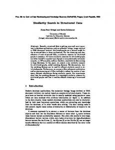
In applications domains like bioinformatics or multimedia data management, objects appear which cannot be described by a single tuple in a relational database. Examples of such data objects are molecules, images or audio data. Those data objects have a complex internal structure, e. g. atoms in a molecule or objects in an image (cf. figure 1.1. Additionally, those objects are often characterized by internal interaction operations, like chemical interactions. To store such objects in relational databases, they have to be decomposed in their substructures which often entails serious performance problems for the database applications. Consequently, the support for complex abstract data types which can be used to describe such objects is essential and lead to the development of object-oriented and object-relational database systems. The internal structure of complex data objects varies from applica-

1.2. CHALLENGES FOR MODERN DATABASE SYSTEMS

5

Figure 1.1: Examples of complex structured data objects: a protein and an image.

tion to application, but often it can be described by using the abstract concepts of graphs and trees. Figure 1.2 shows two examples of such data objects. The support of complex graphs-structured data types is an important feature of today’s database systems. Data objects of the above type are naturally modeled as attributed graphs or trees and, therefore, those data types are the main focus of this thesis. O

C C

C C

C

O

C C

O H

C C H

O

William Shakespeare Romeo and Juliette

H

drama ...

Figure 1.2: Graph structured and tree structured objects: a molecule and an XML document.

6

Figure


1.3:

Growth

of

the

GenBank

database

(source:

http://www.ncbi.nlm.nih.gov).

1.2.2

The Fast Growing Size of Databases

Another problem in conjunction with modern databases is their fast growing size. The amount of data produced in areas like bioinformatics [BKML+ 03, BWF+ 00] or high energy physics [Jar03] are enormous. Figure 1.3 shows the growth of the GenBank database [BKML+ 03], a database of genetic sequences, in the past twenty years. What has to be noted is that the size of this database doubled almost every twelve months in the past ten years.

1.2. CHALLENGES FOR MODERN DATABASE SYSTEMS

7

Figure 1.4: The KDD process.

According to Moore’s Law, the performance of computer chips doubles every two years which means that the size of GenBank grows faster than the computing power. Consequently, it is vital to develop more efficient algorithms for databases like GenBank in order to ensure effective knowledge discovery in those databases.

1.2.3

New Database Tasks

A third challenge for modern database systems is the support for new tasks like Internet connectivity and, especially, knowledge discovery in databases (KDD). KDD is the process of extracting new, valid and potentially useful knowledge from databases [FPSS96]. Particularly in a world of large and fast growing databases, a process to automatically or at least semi-automatically extract knowledge from those databases is essential. The KDD process, as defined by Fayyad, Piatetsky-Shapiro and Smyth [FPSS96], has several steps which are depicted in figure 1.4. After a selection and preprocessing of the relevant data, it is transformed in a suitable format. In the data mining step, patterns in the

8


data are extracted and later evluated by the user, to gain knowlwedge. At the center of the KDD process is the data mining step, where the automatic detection of the information takes place. Several different subtasks of data mining have been identified, including clustering and object classification. Clustering is the task of grouping objects, where the similarity of objects within a group has to be maximized, while the similarity of objects in different groups has to be minimized. Obviously, the clustering of objects in a database depends on efficient and effective methods to identify similar objects in the database, or in other words, it depends on similarity search methods. But those methods also play a major role in object classification, where new objects have to be assigned to a class based on the knowledge extracted from a database of already classified objects. In this context, so-called nearest neighbor classifiers were successfully used, which assign an object to the class of its nearest neighbors in the database. This means that similarity search is an important basic technique for data mining in general.

1.3

Graphs

The previous sections can be summarized by the statement that there is a strong need to develop effective and efficient similarity search methods for structured data in large databases. Structured data in this context means data that is modeled as attributed graphs or attributed trees. In this section we present the definitions of several important terms,

1.3. GRAPHS

9

starting with the definition of graphs. Since we use graphs to model finite data objects, we consider only finite graphs. Definition 1.1 (graph, attributed graph) A graph G(V, E) is a pair of a finite set of vertices V and a finite set of unordered pairs E ⊆ V × V , called edges. An attributed graph is a graph whose vertices each have associated a vector of attributes Av ⊂ IRn and whose edges each have associated a vector of attributes Ae ⊂ IRm , with n, m ∈ IN . A subgraph of a graph G(V, E) is a graph G0 = (V 0 , E 0 ) where V 0 ⊆ V and the following condition holds: ∀e ∈ E : e = (v, w), v ∈ V 0 , w ∈ V 0 ⇒ e ∈ E 0 A graph G(V, E) is said to be directed if all elements of E are ordered pairs. Although we define attributes to be real numbers, this type of attributed graph is not limited to real numbers since categorical attributes can be mapped into IR.

1.3.1

Important Properties of Graphs

The different similarity models and algorithms in the following chapters are all based on the graph properties which we define in this section. There are several figures used to describe graphs, e.g.chromatic number or girth. Most important for the discussions in the following chapters are the order and size of a graph and the degree of a vertex.

10


Definition 1.2 (order, size, degree) Let there be a graph G(V, E) . The number of vertices of G, denoted as |V |, is called the order of G. The number of edges of G, denoted as |E|, is called the size of G. An edge e = (v, w) is called incident to the vertices v and w. Two vertices are said to be adjacent if there exists an edge that is incident to both of them. The number of edges incident to a vertex v is called the degree of v, denoted by degree(v). Another important property of a graph is, whether it is connected or not. Definition 1.3 (connectedness) A walk from vertex vi to vertex vj in a graph is an alternating sequence hv1 , ei+1 , vi+1 , ei+2 , . . . , vj−1 , ej , vj i of vertices and edges in the graph, such that ek = (vk−1 , vk ) for k = i+1, . . . , j. A graph G(V, E) is said to be connected, if G contains a walk between each pair of vertices v and w with v, w ∈ V In many application domains objects contain circle-like structures, as for example the molecule in figure 1.2. Therefore, the notion of a cycle in a graph is important. Definition 1.4 (cyclic graph) A walk is said to be a path if it does not contain any vertex twice. A graph is said to contain a cycle if it contains a path with more than three vertices and an edge incident to the first and to the last vertex on the path. For the similarity model presented in chapter 7, the concept of a bipartite graph is essential.

1.3. GRAPHS

11

Figure 1.5: A bipartite graph.

Definition 1.5 (bipartite graph) A graph G(V, E) is said to be bipartite if V can be decomposed into two subsets U and W , such that for all (v, w) ∈ E, v ∈ U and w ∈ W or v ∈ W and w ∈ U . G is said to complete bipartite if for all v ∈ U, w ∈ W : (v, w) ∈ E. Figure 1.5 shows a bipartite graph. Trees are a very important type of graph and, therefore, we will discuss similarity of trees more thoroughly in chapter 6. In discrete mathematics trees are usually defined as undirected, acyclic and connected graphs and trees with a designated root vertex are seen as a special type of tree. Other than in mathematics, we define trees to be directed and rooted. This definition is the most common in computer science and takes into account that by far the most treestructured data objects in computer science are directed and rooted. Therefore, we define this case as the general one. Definition 1.6 A connected and directed graph G(V, E) is called a tree if the underlying undirected graph is acyclic and there is a special

12


vertex r ∈ V , called the root of the tree for which there exists a path from r to all other vertices v ∈ V . The vertices in a tree are usually called nodes.

1.3.2

Storing Graphs

Storing graphs in a database can basically be done in two ways which are the use of adjacency matrices or of adjacency lists. While vertices are always stored in an appropriate structure for sets, the two approaches differ in the way edges are stored. When using an adjacency matrix to store a graph with n vertices, a n × n-matrix is created and an entry in this matrix at position (i, j) that differs from zero means that there is an edge between the vertices i and j. The advantage of this approach is that it can be tested very efficiently if two vertices are adjacent and, therefore, navigation through the graph can be done very efficiently. The high storage utilization even for sparse graphs is one of the disadvantages of the adjacency matrix approach. Another drawback of this approach is that an attribute vector associated with an edge cannot be stored together with that edge since the edges are not materialized. When using adjacency lists, a list containing all vertices which are adjacent to v is stored for each vertex v in a graph. With this approach the complete adjacency list of a vertex has to be scanned in the worst case, in order to decide whether two vertices are adjacent or not. Therefore, navigation through the graph is rather expensive. Nevertheless, adjacency lists have the advantage that edge attributes can be stored with the respective entry in an adjacency list and, con-

1.4. EXAMPLE APPLICATIONS

13

sequently, can be retrieved efficiently together with the accompanying edge. For this reason, we prefer the adjacency list approach for our implementations.

1.4

Example Applications

Structured data appears in many application domains, for eample in face recognition [WFKvdM97], shape retrieval [SKK01] or biochemistry [BKAW97]. In this section we describe two applications from the image retrieval and bioinformatics domain which are both based on structured data. The data and the requirements of those applications will be used throughout the thesis to evaluate the similarity search models and algorithms that are presented.

1.4.1

Content-Based Image Similarity

The task of content-based image similarity search is to find all similar or the most similar images in the database relative to a given query image. For content-based image similarity not only colors or shapes are important, but also the topological relation between shapes is of importance. When searching for images, e.g.depicting cars, it is not sufficient to find images containing tires, windows and car bodies. Instead, the parts have to be in the correct relative position to each other. This topological relation of the parts is modeled as an attributed graph in our example application. The structure of an image is extracted automatically in a two-step process. To extract the structure data from an image, it is segmented,

14


Figure 1.6: An image and the extracted graph. The size attribute is not shown.

using an appropriate segmentation algorithm. While there could be used virtually any algorithm that produces a segmentation of an image, we use a region-growing algorithm which divides the image into arbitrarily shaped, connected regions of similar color. The second step of the structure extraction process is the construction of a graph from the image segments, which is also done in a two-step process. First, a vertex is generated for each segment and is associated with a vector containing the segment’s attributes. Those attributes are the average color of the segment, the size relative to the image size and in some cases also the horizontal and vertical extension of the segment relative to the image extensions. In the second step, the vertices that represent neighboring segments are connected by edges. This way, a graph is created which represents the topological relations of the segments present in an image. Figure 1.6 shows an example of an image and the


15

number

order

size

of graphs

min.

avg.

max.

min.

avg.

max

TV images

9898

1

9.03

28

0

11.71

74

commercial color images

8536

1

47.76

325

0

90.03

548

pictographs

705

2

10.97

93

1

9.16

92

Table 1.1: Statistics of the image data sets. extracted graph. We applied our structure extraction method to various sets of images, whic are a set of TV snapshots, commercially available color images and black and white pictographs. Table 1.1 shows some statistics about the resulting databases of graphs.

1.4.2

Bioinformatics

The research work presented in this thesis was mainly done with funding from the German Science Foundation (DFG) under grant number KR 670/9-1 and KR 670/9-2 and with funding from the German Ministry of Education and Research (BMBF) under grant number 031U112F. Those projects were concerned with the 1:n-docking of flexible proteins and the functional classification of protein structures. Consequently, the second application example is from the field of bioinformatics and deals with protein similarity search and protein docking. Proteins are large biomolecules consisting of several hundred up to several thousand atoms. They are important building blocks of any living organism, being responsible for the stability of the organism as

16


Figure 1.7: Example of two docking proteins.

well as for the regulation of most processes in an organism. All those functions are performed through the docking of proteins which is the building of a loose compound by two or more proteins. Therefore, questions like with which other proteins a query protein can dock and how the docking complex looks like are very important for biological and medical research, for example in the field of drug design. Figure 1.7 illustrates the docking of two proteins. Additionally, similarity search in protein structures is an important tool for biologists to determine the function of newly detected proteins. For this task, it has to be searched for so-called homologous proteins, i.e. structurally similar proteins with known function in a database. Studies have shown that homologous proteins usually also have similar function and, consequently, it can be inferred that a newly detected protein has a similar function as homologous pro-


17

Figure 1.8: Functional classification of proteins.

teins from the database. This way a functional classification of newly detected proteins is achieved. The process of functional classification of proteins is shown in figure 1.8. The unclassified protein is transformed into a suitable representation for the classification algorithm. For structured data this is a graph representation. Afterwards, the classification takes place based on a similarity search in the database of proteins with known function. For the function of a protein, two properties are important, which are the shape and the chemical properties of the protein surface. Only if the geometric shape of the surfaces are inverse to each other and the chemical properties are appropriate, two proteins can dock. A consequence for protein models is that the model has to be capable of representing the structure of the surface as well as certain biochemical attributes of a protein. Attributed graphs are one way to fulfill this requirement. To evaluate our similarity search methods in the context of protein docking and functional classification of proteins, we used the threedimensional protein structure data from the PDB database [BWF+ 00]

18


which is one of the most important sources of protein data in molecular biology. Our first application is a model for protein docking which is based on a graph representation of potential docking sites, i.e. a region on the protein surface that may take part in a docking of two proteins. To identify those potential docking sites, we used a technique presented by Meier et al. [MAH+ 95] which produces a set of potential docking sites for a protein, each represented as a set of surface points called a region. Those regions are transformed into graphs in a two-step process. First, critical points, which are points either in very concave or in very convex parts of the region, are identified. This identificaton is done be searching points with high or low solid angle values. The solid angle of a point is the percentage of a probe sphere around the critical point which is filled by protein surface points. Each critical point is represented by one vertex in the created graph. For our experiments, we concentrated on the geometric aspects of the protein docking problem. Therefore, no biochemical attributes have been integrated so far. Instead, each vertex is assigned the solid angle value of the critical point as an attribute. In the second step of the graph extraction process, those vertices representing neighboring critical points are connected by edges. The edges have associated the Euclidean distance of the critical points which are connected by the edge. It has to be noted that this process does not always yield connected graphs. Instead, a region can be modeled by a set of connected components. Therefore, the similarity search methods applied to this problem have to be capable of handling

1.5. CONCLUSIONS AND OUTLINE OF THE THESIS number

order

19 size

of graphs

min.

avg.

max.

min.

avg.

max.

functional classification data

800

2

68.89

134

0

90.75

440

docking data

3480

7

22.24

44

6

85.17

268

Table 1.2: Statistics of the protein data sets. objects modeled in this way. For the functional classification problem, entire proteins from the PDB are modeled by attributed graphs. The generation of the graphs for the proteins is also done in several steps. First, potential docking sites are identified, using the previously technique of Meier et al., again. Afterwards, one vertex is generated for each potential docking site, which has the site’s hydrophobicity and its character as attributes. The hydrophobicity of an protein surface region is a biochemical property of the region which has been proven to play a major role in protein docking. The character of a region is a value representing, whether the region is concave, convex or flat. The table 1.2 summarizes some of the characteristics of the data sets we used in our experiments.

1.5

Conclusions and Outline of the Thesis

In this chapter, we presented some of the challenges of modern database systems. Those challenges include support for complex data types, the rapidly increasing size of databases and new applications for database systems. We demonstrated that there is a need for efficient

20


and effective similarity search methods in large databases of graph structured data. The aim of this thesis is to improve the efficiency of known similarity search methods and provide new approaches to solve the efficiency and effectiveness problems of the existing methods. The thesis is organized as follows: In chapter 2, we present important concepts of similarity search. This includes query types, similarity models and index structures to support efficient query processing in similarity search systems. Furthermore, we develop a set of requirements which similarity search methods for attributed graphs have to fulfill in order to meet the demands of modern database applications. Afterwards, the main part of the thesis begins with a discussion of existing similarity search methods for graphs in chapter 3. Among the presented measures, the edit distance stands out, since it is common in several application domains. Consequently, the strengths and weaknesses of the edit distance are discussed in detail in chapter 4. Following the discussion of existing similarity search measures for graphs, we present techniques to improve the query processing time when the edit distance is used as similarity measure. Our experimental evaluation of those techniques also shows that the edit distance can only be used for large databases if the number of distance calculations is kept at a minimum. In chapter 6, techniques for efficient similarity search in large databases of attributed trees are presented. Attributed trees are an important subclass of attributed graphs and are used in applications with hierarchically structured data objects. In this chapter, we also present

1.5. CONCLUSIONS AND OUTLINE OF THE THESIS

21

an application from the area of web site mining. A new similarity measure for attributed graphs, called the edge matching distance, is introduced in chapter 7. We demonstrate the effectiveness of the edge matching distance in experiments and provide new methods for efficient similarity search in large databases of attributed graphs using the edge matching distance as similarity measure. The thesis closes with a conclusion summarizing the main contribution of this work. Additionally, an outlook on future research directions is given.

22


Chapter 2

Similarity Search In the previous chapter, the relevance of similarity search for modern database applications was already highlighted. The basic task of a similarity search application is to find objects in the database which are similar to a query object. In this chapter, we will discuss the different aspects of this task.

2.1

Similarity Models

The first important aspect of similarity search is the concept of similarity itself. A formal concept of similarity is a necessary basis for any application in this field. In the literature, two concepts of similarity have been applied successfully which are the feature vector approach and the concept of distance-based similarity. We will present the two concepts in this section and discuss invariance and adaptability issues of similarity models. 23

24

CHAPTER 2. SIMILARITY SEARCH

object space

feature space

Figure 2.1: Similarity based on the feature vector approach.

2.1.1

The Feature Vector Approach

A very common way to define the similarity of objects is the feature vector approach. For this approach, a domain expert chooses a set of single-valued object features that describe an object from that application domain. Those features span a so-called feature space and objects are represented as points in this space. This is done by creating a feature vector for each object which contains the feature values of the specific object. Then, the similarity or dissimilarity of two objects is defined as their distance in the feature space. The feature vector approach for similarity, whose idea is illustrated in figure 2.1, has been successfully applied in several application domains like medical imaging [KSF+ 98] and protein similarity [AKKT99]. To determine the distance between two points in the feature space, several measures are used. Most often it is a variant of the Lp -norms,

2.1. SIMILARITY MODELS

25

which are defined as follows: Definition 2.1 (Lp -norms) Let there be two vectors x = (x1 , . . . , xn ), x ∈ IRn , and y = (y1 , . . . , yn ), y ∈ IRn . The Lp -norms between x and y are defined as:

n X 1 Lp (x, y) = ( |xi − yi |p ) p i=1

For p = 1 and p = 2 the Lp -norms are the well-known Manhattan distance and the Euclidean distance, respectively. Most often, the Euclidean distance is used in similarity search applications based on the feature vector approach. A problem of the Lp -norms is that all dimensions of the feature space are considered to be independent of each other. Consequently, no relationships between the features, for example substitutability, may be regarded by the similarity process. But often such relationships exist, like in the case of color features where orange is certainly more similar to red or yellow than to blue. To overcome this disadvantage, Niblack et al. [NBE+ 93] suggested to use the quadratic form distance instead of the usual Euclidean distance. The quadratic form distance of two vectors x and y is defined as d2A (x, y) = (x − y) · A · (x − y)T where A is a positive definite similarity matrix and (x−y)T is the transpose of (x − y). When using the identity matrix as similarity matrix, the quadratic form distance becomes the classic Euclidean distance since (L2 (x, y))2 = (x − y) · (x − y)T

26

CHAPTER 2. SIMILARITY SEARCH By altering the similarity matrix A, it is possible to express re-

lationships between the dimensions of the feature space which is the desired effect. For methods to ensure efficient query processing with the quadratic form distance see [Sei97]. Feature Vectors of Attributed Graphs Because of the set-like internal structure of a graph it is difficult, to apply the feature vector approach to data modeled as attributed graphs. This internal structure prevents a unique describtion of the graph structure with few feature values. The same is the case for the attribute part of an attributed graph. Consequently, many features have to be extracted from a graph in order to yield a description with sufficient discriminatory power to distinguish between separate objects and leads to extremely high-dimensional feature vectors. But the high dimensionality of the feature vectors can make efficient similarity search in the database impossible due to a number of effects. For example, an increasing dimensionality leads to a larger volume of the data space and to higher distances between the data objects. Those and other effects are usually described by the term ’curse of dimensionality’. Additionally, when coosing the features one has to take into account that any of the simple Lp -norms or the quadratic forms distance yield sensible results for a similarity search. This fact even worsens the problem of picking the right features. The distance-based similarity model, which we describe in the following section, avoids the choice of any features at all.


d

27

nce ista

.5

=2

nce

dista

nce =

=1

dista

3

object space

Figure 2.2: The concept of distance-based similarity.

2.1.2

Distance-Based Similarity

The distance-based similarity model is a generalization of the feature vector model. Instead of transforming the data objects into a feature space and measuring the distance of the objects in the feature space, a distance measure for the data objects themselves is defined. This means that no feature extraction and no choice of features is necessary. Furthermore, a distance measure which is defined for the structured data objects can take all object properties into account. The concept of distance-based similarity is illustrated in figure 2.2. Obviously, the increased flexibility also means a higher complexity, since the complete objects have to be managed and, therefore, the computational complexity of the similarity measure has to be chosen carefully to ensure efficiency.

28

CHAPTER 2. SIMILARITY SEARCH The great flexibility of the distance-based approach is founded in

the similarity distance measure. If O is the domain of the objects 0 in the database, a similarity distance dsim : O × O 7→ IR+ is needed

which means the only restriction for the similarity measure is positivity. While this very high flexibility may be useful in certain special applications, it usually makes sense to impose some restrictions on the similarity distance measure in order to ensure that efficient query processing is possible. The restrictions imposed on the similarity measure can be summarized by demanding the measure to be a metric, which also justifies to call it a similarity distance. This requirment implies that the similarty measure has to fulfill the four metric properties: 1. Positivity: ∀x, y : dsim (x, y) ≥ 0 2. Definiteness: ∀x, y : dsim (x, y) = 0 ⇔ x = y 3. Symmetry: ∀x, y : dsim (x, y) = dsim (y, x) 4. Triangle inequality: ∀x, y, z : dsim (x, z) ≤ dsim (x, y) + dsim (y, z) The requirements of positivity and definiteness for the similarity distance reflect the idea that a low distance means high similarity and, therefore, identical objects should be assigned the lowest possible similarity distance. The idea that objects are mutually similar is expressed by the symmetry requirement. The triangle inequality ensures that no object can be very similar to two very dissimilar objects at the same time.


29

Demanding metric properties from a similarity distance also has the advantage that efficient access methods and search algorithms can be applied, as described in section 2.3.

2.1.3

Invariance against Transformations

Another important topic in the context of similarity models is robustness against geometric transformations of the original data objects. Similarity search is often done in databases containing geometric descriptions of real-world objects, like molecules, images or mechanical parts. Our example applications are also from such application domains, so we discuss the robustness against geometric transformations. By ’robustness against geometric transformations’ we mean invariance against transformations such as translation, rotation or scaling. Depending on the application, specific invariances are either necessary or have to be avoided. An example application is similarity search in a database of proteins. Since there is no standard position or orientation of proteins defined, the proteins in the database have arbitrary orientation and position in 3D space. Consequently, invariance against translation and rotation are essential to identify similar proteins. On the other hand, invariance against scaling is unwanted, because proteins with different size but similar shape have different properties and should not be considered as similar. When modeling objects as attributed graphs, invariance against rotation, scaling, transformation or mirror reflection are fulfilled automatically by the model, since position information is not included in the graph model. If these invariances are unwanted, the position

30


information can easily be included via attributes. An example for this technique is the data model for proteins which we described for an protein docking application in section 1.4.2. The protein surfaces are modeled as vertices, representing critical points on the surface which are connected by edges, carrying the Euclidean distance of the critical points as attributes. Since only the information about the relative positions of the critical points is stored in the graph structure, the model is obviously invariant against translation and rotation. But invariance against scaling is not fulfilled, assuming that the similarity distance measure takes the edge attribute into account, which is not invariant against scaling. This example demonstrates another advantage of modeling real-world objects as attributed graphs.

2.1.4

Adaptable Similarity Search

In the previous sections, the adaptability of the different models and techniques was highlighted several times. This adaptability is of great importance for similarity search applications, because the exact definition of what is to be considered similar depends on two factors, which are the application domain and the user. An example of application requirements is our protein docking application, where we saw that invariance against translation and rotation is necessary while invariance against scaling has to be avoided. Therefore, the similarity model and the similarity measure have to provide enough flexibility to allow adaption to the specific needs of an application. Apart from the application needs, the notion of similarity can differ between individual users or even for a single user in different situations.


31

Similarity search is often an explorative process during which the user refines his notion of similarity more and more. The adaption to the application’s needs can be considered during the design phase of the application and an adaption of the similarity model is possible in this phase. This approach can not be followed for the adaption to the users needs, since those can change between two similarity queries. Consequently, the similarity measure has to provide the flexibility to allow the necessary adaption at runtime. Obviously, this should be possible with as little influence on query runtimes as possible, to support the explorative nature of the similarity search process. We already discussed the quadratic form distance as an example for such a measure. In [Sei97] efficient query processing techniques are presented which allow an adaption of the similarity matrix for this measure without influencing the processing time negatively. But for a purposeful adaption of the similarity measure, another point gains importance. The user has to be able to understand why objects are considered similar by the application in order to change parameters appropriately. Consequently, the user should be provided with an explanation of the similarity distance value to support his understanding. Obviously, a simple numerical value does not fulfill this requirement. Instead, an explanation how this value comes about is necessary, which is preferably presented visually for a quick and easy understanding.

32

2.2


Similarity Query Types

In similarity search applications, the query types differ from those in standard database applications. Questions like which database objects are most similar to a query object or which database objects are similar to a certain degree, cannot be answered by using exactmatch or partial-match queries. Instead, query algorithms returning database objects in a certain similarity distance to a query object are needed. In this section, we will present those query types which are most important in similarity search applications. For the presentation of the query types, we assume that O is the universe of all objects that may appear in a database and that a similarity distance function 0 is defined on the universe O. Furthermore, we dsim : O × O 7→ IR+

presume that there is a database DB ⊆ O given. It has to be noted that we do not assume a specific similarity model and the discussions below hold for applications based on the feature vector model as well as for applications using the distance-based similarity model.

2.2.1

Similarity Range Query

A basic task in similarity search is to find all objects which are within a certain similarity distance from a query object. Examples where this problem has to be solved are density-based clustering methods like DBSCAN [EKSX96] or OPTICS [ABKS99]. In density-based clustering, an object o is put into a cluster if there are enough other objects within a predefined similarity distance to o. To determine a clustering of a database, for each object in the database the objects within the

2.2. SIMILARITY QUERY TYPES

33

q

Figure 2.3: Result of a range query for object q.

predefined similarity distance have to be found. This is done by using similarity range queries. Figure 2.3 illustrates the idea of the similarity range query. With this intuitive understanding of a similarity range query, we can define it formally in the following way: Definition 2.2 (similarity range query) For a query object q ∈ O 0 and a query range ∈ IR+ , the result of a similarity range query is

defined as sim (q) = {o ∈ DB|dsim (q, o) ≤ } Obviously, with this definition the number of results for a similarity range query is not fixed in advance, but can be anything between zero and the size of the database. Consequently, the choice of an inappropriate value for the query range leads to very few or too many query results and it remains to the user to re-run the query

34


q

Figure 2.4: Result of a nearest-neighbor query with two nearest neighbors for query object q. The gray circle represents the equivalent range query.

with an adapted query range. This problem is another reason, why a similarity measure should also include an explanation of the distance value to allow an adaption of the query range.

2.2.2

Nearest-Neighbor Query

Another important task in similarity search applications is to find the database object which is most similar to a query object. An example for this query type is to find the most similar protein with known function in a database, given a query protein with unknown function. This type of query is called nearest-neighbor query and can be defined informally as the task to find the database object with the smallest similarity distance to the query object. Figure 2.4 illustrates the idea of the nearest-neighbor query.


35

But this informal definition ignores the problem that the database object with the smallest distance may not be unique. In this case, one of the objects with the smallest similarity distance to the query object may be chosen randomly. But then query processing is no longer deterministic and important results may be missed. Therefore, the nearest-neighbor query is defined in a way that allows a set of results which possibly contains more than one element. Definition 2.3 (nearest-neighbor query) For a query object q, the result of a nearest-neighbor query is defined as simnn (q) = {o ∈ DB|∀p ∈ DB : dsim (q, o) ≤ dsim (q, p)} With this definition, it remains to the user to resolve the ambiguity problem, but still, the result is at least a non-empty set. Especially when exploring a database manually, the guaranteed result is an advantage over the similarity range query for the user. The following lemma reveals another relationship between nearest-neighbor and range queries. Lemma 2.1 For every query object q ∈ O, the following holds: nn = min{dsim (q, o), o ∈ DB} ⇒ simnn (q) = simnn (q) Proof. For every object o ∈ DB the following equivalences hold: o ∈ simnn (q) ⇔ ∀p ∈ DB : dsim (q, o) ≤ dsim (q, p) ⇔ dsim (q, o) ≤ min{dsim (q, p), p ∈ DB}

36

CHAPTER 2. SIMILARITY SEARCH ⇔ dsim (q, o) ≤ nn ⇔ o ∈ simnn (q) The above lemma shows that every nearest-neighbor query can

be transformed into a similarity range query, although the nearestneighbor distance nn is generally not known in advance.

2.2.3

k-Nearest-Neighbor Query

The k-nearest-neighbor query is an extension of the nearest-neighbor query in case, a result set with more than one element is desired. An example of such a case is the functional classification of proteins. To improve classification accuracy for nearest-neighbor classification, a protein is not assigned to the functional class of the most similar protein in the database but to the class of the majority of the k most similar proteins. The idea of the k-nearest-neighbor query is illustrated in figure 2.5. Like the nearest neighbor for a query object, the k-th nearest neighbor may not be unique and, therefore, the result of a k-nearest-neighbor query may contain more than k elements.

Definition 2.4 (k-nearest-neighbor query) For every query object q ∈ O and a query parameter k, the result of a k-nearest-neighbor query is defined as


37

q

Figure 2.5: Result of a k-nearest-neighbor query for object q and k = 5. The gray circle represents the equivalent range query.

simknn (q) = {o | o ∈ Nk (q) ⊆ DB ∧ ∀o ∈ Nk (q), ∀p ∈ (DB − Nk (q)) : dsim (q, o) < dsim (q, p)} Obviously, lemma 2.1 holds analogously for the k-nearest-neighbor query which means that every k-nearest-neighbor query can also be transformed into a similarity range query with the same result.

2.2.4

Similarity Ranking Query

A final important similarity query type is the similarity ranking query which is needed in cases where the exact number of desired results is not known in advance. The idea of this query type is to iteratively retrieve the next closest objects of a query object from the database, starting

38


at the nearest neighbor. This type of query appears, for example when the user interactively explores the database and retrieves the nearest neighbors of a query object one after another. Such queries could be done by issuing k-nearest-neighbor queries with increasing parameter k. But this would result in retrieving the nearest neighbor and other objects several times, i.e. again and again for each k-nearest-neighbor query. Therefore, an algorithm for similarity ranking queries should not start over again for each request of a new object and should not perform all the similarity searching while processing the first request to ensure interactive response times. Hijaltason and Samet presented an algorithm with those properties in [HS95].

2.3

Efficient Similarity Search

The size of modern databases and the complexity of the similarity searching task make efficiency an important issue for any similarity search application. In this section, we will present two techniques to speed up the query processing in similarity search applications. The two techniques, the use of index structures, and the use of a multi-step query processing architecture, are not meant to be mutually exclusive. Instead, they can both be applied in parallel or at different stages of the query processing.

2.3.1

Index Structures

The use of index structures is a standard technique to improve query processing times in database systems. Numerous different index struc-

2.3. EFFICIENT SIMILARITY SEARCH

39

tures have been proposed for many different data types and applications. For similarity search in structured data two types of structures are important: structures for high-dimensional vector spaces and for metric spaces. The first category is useful whenever the feature vector approach is used as similarity model, but we will see in the second part of the thesis that it can also be applied to speed up certain subtasks when using the distance-based similarity model. Metric index structures, on the other hand, can be applied if the distance-based similarity model is chosen, provided that the similarity measure fulfills the metric properties. But especially for the distancebased similarity model, where the similarity measure is often complex, speeding up the query processing is essential. In the following, we will present the principles of important index structures for vector spaces as well as metric spaces. Indexing Vector Spaces The two main paradigms for index structures are hashing and tree structures. While there exist hashing approaches for vector spaces [NHS84, KS86], the vast majority of index structures for vector spaces are hierarchical data organizing structures. The idea behind those structures is to organize the vector data in a tree like directory to ensure logarithmic time complexity of index updates and search accesses. To achieve a tree structure for the index, the data vectors are grouped into pages which are described by a page region covering the entire subspace occupied by the data vectors on the page. The data pages are grouped into directory pages in the same manner until this recursive

40


process yields a single root page. The many index structures following this approach differ in the shape and size of the page regions, the strategy for splitting pages and the insertion strategies. Examples of index structures following this paradigm are, among many others, the members of the R-tree family [Gut84, BKSS90], the X-tree variants [BKK96, Sch99] and the IQ-tree [BBJ+ 00]. Indexing Metric Spaces Index structures for metric spaces are more general than structures for vector spaces in the sense that they can also be applied to vector spaces, since every vector space is also a metric space. Like structures for vector spaces, index structures for metric spaces also group the data objects into data pages. But since there is only a distance measure given between pairs of objects, no arbitrarily formed page regions are possible. The limitation of the distance measure results in ball-shaped or ring-shaped page regions. For the description of the page regions, one or more representatives from the data objects together with a radius have to be chosen. The many index structures for metric spaces mainly differ in the way, those representatives are chosen. Examples of index structures for metric spaces are GNAT [Bri95] or the family of ¨ vantage-point trees [Uhl, Yia93, BO97]. Chávez et al. give an overview over existing approaches for indexing metric spaces in [CNBYM01]. Since even in data mining applications regular updates of the database are common, dynamic index structures for metric spaces are the most important variants for our similarity search applications. The M-tree [CPZ97] and its variant the Slim-tree [TTSF00] are specifically

2.3. EFFICIENT SIMILARITY SEARCH

41

designed to allow dynamic updates. Furthermore, those structures are also designed to reduce the number of similarity distance calculations which is especially important for complex similarity measures like they are common for structured data. Therefore, we will compare our techniques for efficient similarity search with the M-tree in the following chapters.

2.3.2

Multi-step Query Processing

The complexity of the similarity distance measure is often a problem for efficient query processing in similarity search applications. Index structures are one way to exclude unnecessary parts of the database from scanning, which reduces the number of necessary similarity distance calculations. Another way to reach this reduction goal is to employ a multi-step query processing architecture. To reduce the number of necessary distance calculations, the query processing in a multi-step query processing architecture, as depicted in figure 2.6, is performed in two or more steps. The first step is a filter step which returns a number of candidate objects from the database. For those candidate objects, the exact similarity distance is then determined in the refinement step and the objects fulfilling the query predicate are reported. To reduce the overall search time, the filter step has to fulfill certain constraints. First, it is essential that the filter predicate is considerably easier to evaluate than the exact similarity measure. Second, a substantial part of the database objects must be filtered out. Obviously, it depends on the complexity of the similarity measure which filter selectivity is sufficient. Only if

42


candidates filter

refinement

result

Figure 2.6: Schema of a multi-step query processing architecture.

both conditions are satisfied, the performance gain through filtering is greater than the cost for the extra processing step. Additionally, the completeness of the filter step is essential. Completeness in this context means that all database objects satisfying the query condition are included in the candidate set or in other words, it must be guaranteed that no false drops occur during the filter step. Available similarity search algorithms guarantee completeness if the distance function in the filter step fulfills the lower-bounding property.

Definition 2.5 (lower-bounding property) For any two objects p and q, a lower-bounding distance function dlb (p, q) in the filter step has to return a value that is not larger than the exact distance de of p and q, i.e. ∀p, q : dlb (p, q) ≤ de (p, q). With a lower-bounding distance function it is possible to safely filter out all database objects which have a filter distance larger than the current query range, because the similarity distance of those objects cannot be less than the query range. Using a multi-step query architecture requires efficient algorithms that actually use the filter steps. Agrawal, Faloutsos and Swami pro-

2.4. REQUIREMENTS FOR SIMILARITY MEASURES

43

posed such an algorithm for range queries [AFS93]. In [SK98] and [KSF+ 98] multi-step algorithms for k-nearest-neighbor search were presented which are optimal in the sense that the minimal number of exact distance calculations are performed during query processing. We employ the latter algorithms in order to ensure efficient query processing whenever applying a multi-step query processing architecture.

2.4

Requirements for Similarity Measures

In the preceeding sections, we discussed several aspects of similarity search applications. From those discussion, we can now derive a few requirements which a similarity measure for structured data should fulfill. All similarity measures in the second part of the thesis are evaluated based on those requirements. One requirement for a similarity measure for structured data is that structural as well as content-related information has to be taken into account. Therefore, the measure should be defined also for attributed graphs and not only for simple graphs. In section 2.1.4, we showed that the similarity measure should be adaptable to the needs of specific applications and to the needs of the users. This adaption should be possible between two queries without negative effects on the performance of the query processing step. Another requirement is closely related to the first one. It is necessary to provide an explanation of the similarity distance value between two data objects, to allow the user a purposeful and easy adaption of the parameters of the similarity distance measure.

44

CHAPTER 2. SIMILARITY SEARCH The final two requirements are concerned with the efficiency of the

query processing in similarity search applications. First, the measure should be of moderate time complexity, since it has to be evaluated often, especially in today’s large and fast growing databases. Finally, a similarity distance measure should be a metric in order to allow the use of index structures and multi-step query processing techniques.

2.5

Conclusion

In this chapter, we discussed several aspects of similarity search applications. In the beginning, we presented two different models for the similarity of objects, namely the feature vector approach and the distance-based model. We discussed the strengths and weaknesses of those models and showed that the distance-based model has advantages especially for structured data. Furthermore, the problems of invariance against transformations and of adaptability to application and user needs were discussed. Afterwards, we presented query types which are important in similarity search applications. Those query types form the basis for the evaluation of the similarity measures in the later chapters. Two different techniques to ensure efficient query processing were presented in section 2.3. Finally, the discussions lead to five requirements which a similarity measure for structured data should fulfill in order to be useful in modern database systems.

Part II

Similarity of Structured Data

45

Chapter 3

Similarity Measures for Graphs Graphs are a very universal and flexible data model and are used in many different application domains. This fact lead to the development of several similarity measures for graphs, which are optimized for different applications and graph types. In this chapter we will discuss such similarity measures for structured data from the literature. The focus of the discussion will be on the requirements for similarity measure that we defined in the preceeding chapter and on the universal usability of the measure for many graph types and applications.

3.1

Measures for Graphs

There exist several similarity measures for graphs. They differ in the types of graphs for which they are defined and whether they take at47

48

CHAPTER 3. SIMILARITY MEASURES FOR GRAPHS

tribute information into account or not. But most of the measures have one thing in common, which is that they are based on some sort of edit operations. The basic idea of all those measures is to define the similarity of graphs based on the effort needed to make the graphs identical. This effort is measured in number of primitive operations which are needed to make the graphs identical. In the following sections will present the similarity measures for graphs from the literature and discuss, how the different approaches define the identity of graphs and the effort to achieve it.

3.1.1

The Edit Distance for Graphs

The edit distance for graphs is an extension of the well known edit distance for strings [Lev66, WF74] to graphs. Sanfeliu and Fu first introduced the edit distance for attributed graphs in [SF83]. The edit distance is a very common similarity measure for graphs and variants of it have been used successfully in many application domains such as face recognition [WFKvdM97] or object recognition [KKV90]. The edit distance between two graphs is the minimum number of edit operations which are necessary to transform the graphs into each other. Edit operations may be the deletion or insertion of vertices or edges or the change of vertex or edge attributes. There exist many variants of the edit distance for graphs which differ in the edit operations that are allowed or whether attributes are considered or not. Due to its great importance, we will discuss the edit distance for graphs more thoroughly in chapter 4, where the edit distance is also defined formally.

3.1. MEASURES FOR GRAPHS

3.1.2

49

The Measure of Papadopoulos and Manolopoulos

In [PM99] Papadopoulos and Manolopoulos present a similarity measure for graphs, which is also based on the concept of edit operations. They propose three different primitive operations, which are vertex insertion, vertex deletion and vertex update. While vertex insertions or deletions have the obvious meaning, the update operation is needed to insert or delete edges incident to a vertex. Additionally they introduce the degree sequence of a graph, i.e. the non-increasing sequence of the degrees of the vertices in a graph. The similarity distance between two graphs is defined as the minimum number of primitive operations which are required so that the two graphs have the same degree sequence. To calculate the similarity measure, the sorted graph histogram is introduced, which is a histogram of the degrees of the vertices in a graph increased by one and sorted in non-increasing order. Papadopoulos and Manolopoulos show that the L1 -distance between two sorted graph histograms equals their similarity distance of the corresponding graphs. Additionally it is proven that the similarity distance satisfies the metric properties. Obviously, the sorted degree histograms of the graphs in a database are of different dimensionality if not all graphs are of the same order. To allow the use of index structures for vector spaces, Papadopoulos and Manolopoulos introduce a histogram folding technique to achieve a constant dimensionality of the histograms for all graphs. To create a folded histogram from a sorted degree histogram, the maximum order

50

hf

} } } } }

hs


Figure 3.1: The histogram folding technique of Papadopoulos and Manolopoulos.

of all graphs in the database and in the queries has to be known in advance. In the beginning the desired dimensionality n of the folded histograms is fixed and for graphs with less vertices than this dimensionality, the sorted degree histogram is simply padded with zeros. In all other cases, a new folded histogram hf is deduced from a sorted degree histogram hs by assigning the sum of the values in the first n-th of the bins in hs to the first bin in hf and so on, until the sum of the values in the last n-th of hs is assigned to the n-th bin of hf . Figure 3.1 illustrates the folding technique.

In [PM99] it is shown that the L1 -distance of two folded histograms is a lower bound for the L1 -distance of the corresponding sorted degree histograms. This allows to use the folded histograms in a filter step of a multi-step query processing architecture. In chapter 6 we will present an alternative folding technique for histograms, which does not require the knowledge of the maximum order of all database and query graphs in advance.


51

Discussion Obviously, the similarity measure of Papadopoulos and Manolopoulos does not take attribute data into account. Furthermore, there is no apparent way to integrate attribute information into the measure without having to develop a new algorithm to calculate the measure. Therefore, this similarity measure is only useful for non-attributed graphs, where only the structure of the data objects influences the similarity of the objects. Adaptability to application and user needs is one of the requirements a similarity measure for structured data has to fulfill. Apparently, the measure of Papadopoulos and Manolopoulos has no adaptable parameters and even the integration of a simple weighting scheme for the primitive operations would require a new algorithm to calculate the measure. The algorithm presented by Papadopoulos and Manolopoulos does not allow to distinguish between the number of different primitive operations which are necessary. Consequently, the measure is adaptable neither to application requirements nor to user needs. An explanation of the similarity distance between two graphs could be provided, since the measure is based on primitive operations. Therefore, one sequence of primitive operations with minimal length, which results in equal degree sequences, could be presented to the user. Unfortunately, the algorithm for calculating the similarity measure only determines the number of necessary primitive operations, but no sequence of this length is acquired. Determining such a sequence would require either a new calculation method for the measure or a separate

52


processing step, which would influence the processing time negatively. The time complexity of the similarity measure, is obviously linear in the maximum order of the graphs. This low time complexity allows to use the measure even for very large databases. Additionally, a filter is available which can be used in a multi-step query processing architecture to further enhance the processing time. Finally, the measure fulfills the metric properties and, therefore, index structures for metric spaces can be used in conjunction with this measure. Summarizing the discussion, it has to be stated that the similarity measure for graphs by Papadopoulos and Manolopoulos fulfills some of the requirements for similarity measures for attributed graphs. Nevertheless, it has severe shortcomings, which limit its usefulness to certain graph types and applications.

3.1.3

The φ-distance Similarity Measure

Another similarity measure for graphs is proposed by Chartrand, Kubicki and Schultz in [CKS98]. This measure is based on mappings between the vertex sets of the graphs, which are compared, and is defined for connected graphs of the same order. Before the similarity measure can be defined, the φ-distance has to be introduced.

Definition 3.1 (φ-distance) Let there be two connected graphs G1 (V1 , E1 ) and G2 (V2 , E2 ) of the same order n and a one-to-one


53

mapping φ : V1 7→ V2 . The φ-distance between G1 and G2 is defined as distφ (G1 , G2 ) =

X

where the sum is taken over all

|lp (u, v) − lp (φu, φv)| n 2

unordered pairs u, v of distinct

vertices in G1 and lp (u, v) is the length of the shortest path between u and v in G1 . The φ-distance similarity measure is defined as follows: Definition 3.2 (φ-distance similarity measure) The

φ-distance

similarity measure between two connected graphs G1 and G2 of the same order is defined as: dφ (G1 , G2 ) = min{distφ (G1 , G2 ) | φ is a one − to − one mapping between V1 and V2 } Chartrand, Kubicki and Schultz show that the φ-distance similarity measure is a metric, but they do not provide an algorithm for calculating the φ-distance similarity measure for graphs. Instead, they present a lower bounding filter for the similarity measure. This filter is based on the total distance td(G) of a connected graph G of order n, which is defined as td(G) = where the sum is taken over all

X n 2

lp (u, v) unordered pairs u, v of distinct

vertices of G. In [CKS98] it is shown that for any two connected graphs G1 and G2 of the same order, the following holds: |td(G1 ) − td(G2 )| ≤ dφ (G1 , G2 )

54

CHAPTER 3. SIMILARITY MEASURES FOR GRAPHS If G1 is a connected spanning subgraph of G2 it even can be shown

that dφ (G1 , G2 ) = td(G1 ) − td(G2 ). Obviously, calculating the total distance of a graph is very time consuming, since n2 many pairs of vertices have to be considered. But this calculation can be done in advance so that the total distance can be used as filter value for a graph. Nevertheless, the calculation of the exact φ-distance measure remains a complex task, since there exist n! one-to-one mappings between the vertex sets of two graphs with order n. Even if an efficient way to find an optimal one-to-one mapping would be known, the distance calculation would still have quadratic time complexity in the order of the graphs.

Discussion The φ-distance similarity measure is only defined for connected graphs of the same order and does not take attribute information into account. The integration of attribute information would be possible by using a distance function which takes attribute information into account instead of the lengths of paths between the pairs of vertices. The choice of this distance function would have to be done carefully in order to preserve the metric property of the φ-distance similarity measure. Nevertheless, the limitation to connected graphs of the same order remains, which limits the applicability of the φ-distance similarity measure to special cases where the requirements are fulfilled.


55

Additionally, the measure has no parameter and, therefore, cannot be adapted to application requirements and user needs. Just like the integration of attribute information, adaptability could be achieved by introducing another distance function for vertex pairs. Again, the choice of this function would have to done with special care to preserve the metric properties. When calculating the φ-distance similarity measure, the requirement of an explanation component could be fulfilled, if the calculation algorithm also determines one of the mappings, which has minimum cost. Obviously, this requirement is only sensible, if adaptability is achieved through an appropriate new distance function. Finally, the time complexity of the measure remains an open issue. But since there is no algorithm with polynomial time complexity known, which calculates the φ-distance similarity measure, a moderate time complexity of this measure cannot be approved. Therefore, the φ-distance similarity measure is limited to very special applications providing data modeled as connected graphs with a small and fixed order.

3.1.4

Similarity Based on the Maximal Common Subgraph

Another similarity measure for attribute graphs was proposed by Bunke and Shearer in [BS98]. Their similarity measure is based on the maximal common subgraph of the two graphs. A graph G is called a common subgraph of two graphs G1 and G2 , if it is a subgraph of G1

56


and G2 , respectively. A common subgraph G of two graphs G1 and G2 is maximal if there exists no other common subgraph of G1 and G2 with a higher order than G. The maximal common subgraph of G1 and G2 is denoted by mcs(G1 , G2 ). The similarity distance by Bunke and Shearer is defined as follows: Definition 3.3 (maximal common subgraph similarity distance) The maximal common subgraph distance between two non-empty graphs G1 and G2 is defined as dmcs (G1 , G2 ) = 1 −

|mcs(G1 , G2 )| max{|G1 |, |G2 |}

It has to be noted that this similarity measure takes attribute information into account, since a graph is only a subgraph if also the attribute information is identical. In [BS98] it is shown that the maximal common subgraph similarity distance is metric. Unfortunately, the maximal common subgraph problem is NP-complete [GJ79]. Consequently, determining the maximal common subgraph similarity distance between two graphs has exponential runtime. An algorithm with worst case time complexity of O(2n ) has been presented also by Shearer and Bunke in [SB97]. Discussion Other than the similarity measure of Papadopoulos and Manolopoulos and the φ-distance similarity measure, the maximal common subgraph similarity distance is defined for attributed graphs and is not restricted to certain graph types.


57

In [BS98], it is stated as a design goal for the development of the measure to avoid the need for a cost function within the similarity measure. As a reason for this, the complexity of choosing the best cost function for edit distance based similarity measure is mentioned. But because of the lack of any cost function, the maximal common subgraph similarity distance cannot be adapted to specific applications and user needs. This fact greatly limits the usability of the measure for many applications. An explanation for the similarity distance could be provided by presenting the maximal common subgraph determined during the calculation. But obviously, this is no longer an important requirement, since the measure has no parameters which can be adapted. While the measure fulfills the metric properties, it can only be calculated with exponential time complexity. Therefore, it does not fulfill the requirement of moderate computational complexity.

3.1.5

Error-Correcting Graph Matching

A problem closely related to similarity search in databases of attributed graphs is graph matching. The term ’graph matching’ is used for the task to find the model graph in a database which corresponds to a query graph. Graph matching is used in face recognition [WFKvdM97], video indexing [SB97] or schema matching [MGMR02]. In ideal situations, graph matching is equivalent to finding a model graph which is isomorphic to the query graph, but in real applications, the data is usually erroneous and incomplete. Consequently, the concept of error-correcting subgraph isomorphism becomes important. It

58


can be described informally as finding the most similar model graph in the database with respect to a query graph. This task is equivalent to a nearest neighbor similarity search. In [Mes96], Messmer presents an algorithm for error-correcting subgraph isomorphism detection in databases of attributed graphs. The algorithm is based on the idea to decompose the model graphs in the database into smaller subgraphs and to represent the database graphs in terms of those subgraphs. Subgraphs which are common to several model graphs are stored only once. This recoding of the database graphs is done in a preprocessing step and should be repeated each time, significant parts of the database are updated, to ensure consistent query response times. During query processing, the subgraph isomorphism determination can be greatly simplified, since matchings with common subgraphs have to be calculated only once. Discussion While error-correcting graph matching is related to the problem of nearest neighbor similarity search, the approaches from this domain are no alternative for similarity measures for attributed graphs. Since all the approaches are optimized to solve only the nearest neighbor problem, other similarity query types are not directly supported. Furthermore, the underlying problem of subgraph isomorphism is NPcomplete and, therefore, all exact graph matching algorithms have exponential time complexity, which prohibits their application to large and even growing databases. Additionally, many graph isomorphism algorithms are based upon

3.2. SIMILARITY MEASURES FOR TREES

59

the edit distance, which can be used directly as similarity measure for attributed graphs.

3.2

Similarity Measures for Trees

It is obvious that every similarity distance measure for attributed graphs can also be used for attributed trees. Nevertheless, several specialized similarity measures for attributed trees have been presented in the literature. One reason for this is the great importance of tree structured data in practice and another reason probably is the high computational complexity of most known similarity measures for attributed graphs. Furthermore, similarity search in tree structured data often requires to take special properties of tree structured data into account. For example, it is usually more important for the similarity of the data objects that the structure and attributes near the root of the tree are similar to each other, than at the leaf level. Due to the great importance of tree structured data in practice, we will thoroughly discuss similarity measures and efficient query processing techniques for tree structured data in chapter 6.

60


Chapter 4

The Edit Distance The most common similarity measure for graphs is certainly the edit distance. This has several reasons. First, it is a very intuitive measure, which means that the user can easily understand how the distance between two objects comes about. As a consequence, the user can adapt parameters systematically if the results of a similarity search are not satisfying. This allows to apply the edit distance in a broad range of applications and strengthens the trust of the user in the results. Furthermore, the calculation of the edit distance also produces a mapping between the vertices of the two compared graphs, which can be visualized for the user. This supports the user in the often explorative similarity search process and again, in adapting the necessary parameters. Another property of the edit distance which also increases its adaptability for different applications and users, is the fact that many variants of the edit distance are available. Those variants are based on different weights for the edit operations, a restriction of the allowed edit operations, or on a combination of those two techniques. 61

62

CHAPTER 4. THE EDIT DISTANCE Because of the importance of the edit distance as a similarity mea-

sure for graphs, we will investigate it more thoroughly in this chapter. After defining the edit distance formally, we will present its important properties and discuss some of its variants. Finally, we will present some results on the time complexity of calculating the edit distance and present an algorithm to calculate this measure.

4.1

The Edit Distance Between Attributed Graphs

While the edit distance is a very intuitive measure, it is nontheless necessary to define exactly what we mean by the term ’edit distance’ between attributed graphs. This is especially important to understand the numerous variants and their specific properties. Important concepts for the definition of the edit distance are single edit operations and sequences of edit operations. Definition 4.1 (edit operation, edit sequence) Let G = (V, E) be an attributed graph. An edit operation is the insertion, the deletion or the change of a label (relabeling) of a vertex or edge in G. The insertion of a vertex or edge x is denoted by (λ → x), the deletion of x is denoted by (x → λ) and the relabeling of x to y is denoted by (x → y). An edit sequence S is a sequence of edit operations, S = he0 , . . . , em i, which can be applied to G. The result of the application of an edit sequence S to a graph G, S(G), is an edited graph G0 . An important detail of this definition is that a single relabeling can

4.1. DEFINITION

63

change the entire label vector of a vertex or edge. Consequently, a single edit operation can change several data values associated with a vertex or node. The next step towards the definition of the edit distance is a cost function for the edit operations. Most variants of the edit distance differ in the cost function they use. Definition 4.2 (edit cost funtion) Each edit operation e is assigned a non-negative cost c(e). The cost of a sequence of edit operations S = he0 , . . . , em i, c(S), is defined as the sum of the cost of each edit P operation in S, i.e. c(S) = m i=0 c(ei ). Before we can define the edit distance, we also have to introduce the concept of graph isomorphism which provides some sort of equivalence of graphs. Definition 4.3 (graph isomorphism) Two graphs G1 = (V1 , E1 ) and G2 = (V2 , E2 ) are isomorphic, denoted by G1 ∼ = G2 , if there is a bijection M ⊆ V1 × V2 such that for every pair of vertices vi , vj ∈ V1 and wi , wj ∈ V2 with (vi , wi ) ∈ M and (vj , wj ) ∈ M , (vi , vj) ∈ E1 if and only if (wi , wj ) ∈ E2 . In such case, M is a graph isomorphism of G1 and G2 . Two attributed graphs G1 and G2 are called isomorphic if there exists a graph isomorphism M of G1 and G2 and the attributes associated with corresponding vertices and edges in M are identical, too. Now, we are finally able to define the edit distance between attributed graphs.

64

CHAPTER 4. THE EDIT DISTANCE

A

B

A

C

G1

C

δedit G1 G2 4

D

C

G2

Figure 4.1: Simple edit distance between two graphs. The distance is calculated with unit cost for all edit operations.

Definition 4.4 (edit distance) The edit distance between two attributed graphs G1 and G2 , dedit (G1 , G2 ), is the minimum cost of all edit sequences S that make G1 and G2 isomorphic: dedit (G1 , G2 ) = min{c(S)|S(G1 ) ∼ = G2 } Figure 4.1 illustrates the idea of the edit distance between two graphs G1 and G2 . Edges and vertices touched by a dashed line are assigned to each other which means that they have to be relabeled if they do not carry the same label. All vertices and edges not touched by a dashed line have to be inserted or deleted, respectively. In the following we call the basis of all variants of the edit distance

4.1. DEFINITION

65

’simple edit distance’. The simple edit distance is uniformly weighted which means that every edit operation is assigned the same cost, which is usually 1. An important property of the simple edit distance and the reason why it is called edit distance is presented in the following theorem. For the theorem it is important to recall that we consider two graphs as identical, if they are isomorphic.

Theorem 4.1 The simple edit distance for attributed graphs is a metric.

Proof. Let G1 , G2 and G3 be attributed graphs. To proof the theorem, we have to show the three metric properties: 1. dedit (G1 , G2 ) ≥ 0 and dedit (G1 , G2 ) = 0 ⇔ G1 = G2 (positivity and definiteness): As the cost for an edit operation is positive, the cost for every edit sequence and, therefore, the edit distance between any two graphs is always positive. As two graphs can only have an edit distance of zero, if they are isomorphic, the second condition is also fulfilled. 2. dedit (G1 , G2 ) = dedit (G2 , G1 ) (symmetry): Assume that dedit (G1 , G2 ) 6= dedit (G2 , G1 ). In this case, there exists an edit sequence S1 = he0 , . . . , em i with S1 (G1 ) ∼ = G2 and c(S1 ) = dedit (G1 , G2 ) 6= dedit (G2 , G1 ). Without loss of generality, we assume that c(S1 ) < dedit (G2 , G1 ). We construct an edit

66

CHAPTER 4. THE EDIT DISTANCE sequence S2 = he00 , . . . , e0m i, with     (b → a) , if em−i = (a → b) e0i = (a → λ) , if em−i = (λ → a)    (λ → b) , if e m−i = (b → λ) The edit sequence S2 is the reversion of sequence S1 . As S1 (G1 ) ∼ = G2 , it is obvious that S2 (G2 ) ∼ = G1 . For the simple edit distance, it is clear that c(S1 ) = c(S2 ) ≥ dedit (G2 , G1 ) which contradicts the assumption. 3. dedit (G1 , G3 ) ≤ dedit (G1 , G2 ) + dedit (G2 , G3 ) (triangle inequality): Assume that dedit (G1 , G3 ) > dedit (G1 , G2 ) + dedit (G2 , G3 ). For each pair of graphs Ga and Gb there exists a cost minimal edit sequence S with S(Ga ) ∼ = Gb . Therefore, there must exist cost minimal edit sequences S1 , S2 and S3 with S1 (G1 ) ∼ = G3 , S2 (G1 ) ∼ = G2 and S3 (G2 ) ∼ = G3 and c(S1 ) > c(S2 )+c(S3 ). But the edit sequence S4 = S2 S3 , c(S4 ) = c(S2 ) + c(S3 ) obviously also makes G1 and G3 isomorphic, i.e S4 (G1 ) ∼ = G3 . This means that c(S2 ) + c(S3 ) = c(S4 ) < c(S1 ) which contradicts the fact that S1 is cost minimal.

4.2

Variants of the Edit Distance

As already mentioned, several variants of the edit distance exist. In this section, we will further investigate a few important examples of those variants.

4.2. VARIANTS OF THE EDIT DISTANCE

4.2.1

67

Weighted Edit Distance

The simplest and most common variant of the edit distance is the weighted edit distance. It differs from the simple edit distance in the cost function for edit operations. While for the simple edit distance, each edit operation is assigned the same cost, in the weighted case, the cost for insertion, deletion and relabeling operations can differ. It is even possible that the cost for an edit operation depends on the individual objects involved in the edit operation. The cost for a relabeling, for example, may be proportional to how much the values of the labels are changed. The use of a weighted edit distance allows to adapt the similarity measure for individual applications and users, but for efficient similarity search, certain properties should be fulfilled by the similarity measure. One of those is the metric property which is a precondition to efficient similarity search algorithms. This raises the question, which properties a cost function for edit operations must have, in order to ensure the metric property of the weighted edit distance. Theorem 4.2 Only if the cost function c fulfills the following two conditions, the resulting weighted edit distance can be a metric: 1. f or all edit operations e : c(e) > 0 2. The cost for deletion and insertion of an object x are identical. Proof. To proof the theorem, we show that the weighted edit distance looses the metric properties if the cost function violates any of the above mentioned properties:

68

CHAPTER 4. THE EDIT DISTANCE 1. f or all edit operation e : c(e) > 0: Assume that this property is violated. The cost function has to be non-negative by definition (see definition 4.2). Therefore, this property can only be violated if there exists an edit operation e with c(e) = 0. But then, it is possible to construct two graphs G1 and G2 with G1 ∼ 6= G2 and e(G1 ) ∼ = G2 . This means that G1 and G2 are not isomorphic but have an edit distance of zero. This violates the metric property of definiteness. 2. The cost for deletion and insertion of an object x are identical: Assume that this property is violated. This means that the operation e of inserting a vertex or edge x, e = (λ → x), and the operation e0 of deleting the same vertex or edge x, e0 = (x → λ), are not assigned the same cost, i.e. c(e) 6= c(e0 ). Obviously, it is possible to construct two graphs G1 and G2 with G1 ∼ 6 = G2 , e(G1 ) ∼ = G2 and G1 ∼ = e0 (G2 ), as the insertion and the deletion of an object are inverse operations. But this means that: dedit (G1 , G2 ) = c(e) 6= c(e0 ) = dedit (G2 , G1 ) Consequently, an edit distance based on such a cost function does not fulfill the metric property of symmetry.

4.2.2

Edit Distance for Trees

In practice, trees are probably the most important subset of graphs, since many data objects have a hierarchical structure. This includes

4.2. VARIANTS OF THE EDIT DISTANCE

69

XML documents, chemical compounds and content-oriented image data. The edit distance for graphs can also be used to measure the similarity of trees, as every tree is also a graph. But often this is unwanted, as in this case the special properties of tree structured data are not taken into account. One such property is the fact that edges in trees usually do not carry any attributes but serve only as a representation of the hierarchical relationship between vertices. Therefore, edit operations for the edit distance for trees are only defined for vertices. The edges adjacent to an edited vertex are implicitly changed. Additionally, insert and delete operations have to be defined in a different way than for graphs. This is due to the fact that trees are always connected and, therefore, the definition of an insert or delete operation has to ensure that a tree remains connected after the operation. This can be guaranteed if the definition of the deletion of non-leaf vertex v implies the deletion of the entire subtree rooted at v. Obviously, such a definition does not yield a useful similarity measure, because with this measure every two trees could be transformed into each other with a maximum of two edit operations. This could be done by deleting the root of one tree and afterwards inserting the entire other tree. Therefore, the insertion and deletion of vertices in a tree are usually defined in the following way: Definition 4.5 (edit operations for trees) Let t be an attributed tree and p a vertex within t. Through the insertion of a vertex n below p, n becomes a successor of p and the elemnts of a subset of p’s successors become successors of n. A deletion is the reverse operation of an insertion.

70

CHAPTER 4. THE EDIT DISTANCE In chapter 6 we will discuss the edit distance for trees and demon-

strate how large databases of tree structured objects can be queried efficiently.

4.2.3

The Measure of Papadopoulos and Manolopoulos

The similarity measure for graphs from Papadopoulos and Manolopoulos [PM99], as already described in section 3.1.2, also represents a special form of edit distance. But in contrast to the measures presented in the previous sections, they do not define an insert or delete operation for edges, but introduce a vertex update operation. Consequently, the deletion of a single edge takes two edit operations which are the update operations for the two incident vertices. Consequently, graphs with different size are considered less similar with Papadopoulos’ and Manolopoulos’ measure than with the normal edit distance. Additionally, the measure is only defined for non-attributed graphs. While this problem could be solved by introducing an appropriate relabeling operation, the resulting measure would be incompatible with the efficient search methods presented in [PM99].

4.3

The Time Complexity of the Edit Distance

In the context of database systems, the computational complexity of a similarity measure is of great interest. As in a database system

4.3. THE TIME COMPLEXITY OF THE EDIT DISTANCE

71

thousands or even millions of objects are stored, the similarity measure potentially has to be evaluated very often during the processing of a single similarity query. The efficiency of the query process is greatly influenced by how fast those evaluations can be made. While there are many different types of edit distance functions, they all have one aspect in common: They all measure the cost for making the compared graphs isomorphic. Therefore, it makes sense to investigate the problem of graph isomorphism before considering the computational complexity of the edit distance as a whole.

4.3.1

Graph Isomorphism

The problem of graph isomorphism is a long studied problem in mathematics and computer science. It is the problem to decide if two graphs are isomorphic according to definition 4.3. The computational complexity of the graph isomorphism problem has been intensely studied [KST93], but so far, it was neither possible to classify it as NP-complete nor to be within P. Jacobo Torán showed in [Tor00] that the graph isomorphism problem is hard under logarithmic space many-one reductions for several complexity classes. While this gives an idea of the complexity of the problem, the general question on the complexity of the graph isomorphism problem remains unanswered. Valiente states that ’[...] graph isomorphism is one of the few NP problems believed neither to be in P nor to be NP-complete.’ ([Val02], p.354). To sum up, there is no algorithm with polynomial runtime for the general graph isomorphism problem known. For some graph classes more efficient algorithms have been pre-

72


sented. Examples are planar graphs [HT71], graphs with bounded degree [Luk82] or graphs with limited eigenvalue multiplicity [BGM82]. However, the general problem remains unsolved.

4.3.2

Time Complexity of the Edit Distance

The fact that the graph isomorphism problem is computationally very complex, has immediate consequences for the complexity of the edit distance problem. As only isomorphic graphs have an edit distance of zero, an efficient algorithm for the edit distance would also provide an efficient isomorphism test for graphs. Consequently, it is not surprising that no efficient algorithm for determining the edit distance between graphs is known. Quite to the contrary, Zhang and colleagues [ZSS92, ZJ94] showed that computing the edit distance between unordered trees is MAX SNP-hard which means that it has no polynomial approximation scheme unless P = N P . But especially in similarity search, it is of great importance that the similarity measure can be evaluated efficiently, as the measure typically has to be evaluated for a large number of objects during one search run. As common data mining techniques issue one similarity query for each database object in the worst case, it becomes clear that the complexity of the edit distance is too high. Consequently, techniques that reduce the complexity of the query processing become indispensible when using the edit distance. A first simple approach to reduce the complexity of the similarity search process when using the edit distance, is to limit the size and order of the graphs. As the worst-case time complexity of an edit

4.3. THE TIME COMPLEXITY OF THE EDIT DISTANCE

73

distance calculation is exponential in the order of the graphs, reducing the order of the graphs in the database would drastically reduce the query evaluation time. But obviously, this approach is unattractive because a limitation of the graph order would also limit the amount of information that can be stored in the graphs. This results in very coarsely modeled database objects and, consequently, in a coarse and often inappropriate similarity model. Apart from that, the number and complexity of the edit distance calculations is not reduced by this approach. The use of a completely different similarity measure, other than the edit distance, can also be considered. We will thoroughly investigate this possibility in chapter 7. As described there, other measures also have certain shortcomings and, therefore, other techniques to reduce the complexity of the similarity distance calculations are called for. A possibility to reduce the number of edit distance calculations during query processing and together with this, the query runtime, is the use of index structures. Most index structures, like the B-tree [BM72], require a complete ordering of the data set or that the data space is a vector space. Examples of the latter category are the many index structures for high-dimensional data, like the R-tree [Gut84], the X-tree [BKK96] or the VA-file [WSB98]. Unfortunately, attributed graphs together with the edit distance do not form a vector space, but as theorem 4.1 shows, they form a metric space. This allows us to use index structures for metric spaces, like the M-tree [CPZ97] or one of ¨ the vantage-point approaches, for example from [Bri95] or [BO97], to speed up similarity search in large databases of attributed graphs with

74


edit distance as similarity measure. To our best knowledge, the M-tree is the only fully dynamic index structure for metric spaces. But as we will show in section 5.3, the use of the M-tree does not reduce the number of necessary distance calculations far enough to allow the use of this similarity measure in large databases of tree-structured objects. All the above mentioned techniques to reduce the complexity of similarity query processing in conjunction with the edit distance have major drawbacks. Therefore, we follow a different approach based on the concept of multi-step query processing, as described in 2.3.2. The necessary filter methods are presented in the following chapter.

4.4

Determining the Edit Distance

Since no efficient algorithms for the calculation of the edit distance are known, general algorithmic paradigms have to be applied to this problem. Dynamic programming and search techniques are common paradigms used to calculate the edit distance between graphs. Here we present a solution based on a search technique, which means we have to find the cost-minimal edit sequence that makes the two compared graphs isomorphic within the space of all possible edit sequences. The basic idea of the algorithm is to find a mapping between the vertices and edges of the two graphs that are compared. All vertices and edges mapped to a corresponding vertex or edge in the other graph have to be relabeled, while vertices and edges without a partner in the other graph have to be inserted or deleted, respectively. Starting with an empty edit sequence, we generate all possible extensions of the

4.4. DETERMINING THE EDIT DISTANCE

75

EDIT DISTANCE(Graph G1 , Graph G2 ){ PriorityQueue sequenceQueue; init sequence queue(); while (complete sequence not found){ s = remove best sequence(sequenceQueue); while (extensions left){ es = extend(s); sequenceQueue.insert(es,cost(es)); } } } Figure 4.2: Algorithm for calculating the edit distance between two graphs current edit sequence and determine their edit cost. The edit sequence with the minimal cost so far is the next one to be extended. This procedure is repeated until all vertices and edges of the smaller graph have either been mapped to a partner or been marked for insertion or deletion. Figure 4.2 shows the algorithm in pseudo-code. This algorithm returns a cost-minimal edit sequence between G1 and G2 . This is ensured by choosing the best edit sequence created so far at every stage, and because the algorithm does not terminate before an edit sequence that makes G1 and G2 isomorphic has been found. Obviously, this algorithm is fast for graphs which have a small edit distance, or in other words, which are similar. For rather dissimilar graphs, the calculation can take very long. But this cannot

76


be completely avoided, because of the complexity of the edit distance measure. Again, that is a reason why unnecessary calculations of the edit distance should be avoided. All the methods presented in the following chapters aim at avoiding unnecessary distance calculations. A major advantage of the above algorithm is its great flexibility. Depending on the exact form of the edit distance that is used as similarity measure, only the cost for matching two vertices has to be adapted. This means that all variants of the edit distance which we investigated can be calculated with this one approach.

4.5

Summary

In this chapter we took a closer look at the edit distance for attributed graphs as a similarity measure for structured data. We showed that the simple edit distance is a metric and presented some conditions which have to be fulfilled by the variants of the edit distance in order to be a metric, too. Additionally, we presented an algorithm which allows to calculate the edit distance and most of its variants. Furthermore, we described some important variants of the edit distance and discussed the computational complexity of the measure. It turns out that the edit distance for graphs is a very common, but extremely complex similarity measure. Therefore, it is necessary to develop alternatives and to speed up the query processing step in order to allow for efficient similarity searching in structured data.

Chapter 5

Efficient Similarity Search with the Edit Distance In the previous chapter, we saw that the edit distance for attributed graphs fulfills almost all of the requirements of a similarity measure which we defined in chapter 3. But unfortunately, the time complexity of the edit distance and its variants is extremely high. In this chapter we will present some techniques to allow efficient similarity search in large databases with the edit distance as similarity measure. 77

78

CHAPTER 5. EDIT DISTANCE SIMILARITY

5.1

Handling the Computational Complexity

There are several ways to deal with similarity measures of high computational complexity. A simple one is to reduce the problem size which means in our case to limit the size and order of the graphs. Obviously, this approach has many disadvantages, since it is not possible to limit the size and order of the object graphs in every application. Besides, this approach does not scale well, because a larger database would require even smaller graphs to maintain acceptable runtimes which eventually leads to a graph that does no longer contain sufficient information. Therefore, the limitation of the graph size and order can only be applied in special cases. Another way to tackle the complexity problem is to use a completely different data model instead of attributed graphs for which similarity measures with lower time complexity are known. But as we already discussed in chapter 1, this is often undesirable or even impossible. A promising approach is the use of index structures in order to reduce the number of necessary edit distance calculations. Obviously, only index structures for metric spaces have to be considered, as the edit distance and attributed graphs only form a metric space but no vector space. In section 2.3.1, such index structures are described. While the use of an index structure reduces the number of necessary distance calculation, this approach still suffers from the time complexity problem in a special way. All the index structures for metric spaces

5.1. HANDLING THE COMPUTATIONAL COMPLEXITY

79

are based on the same idea. Certain objects from the database are chosen as routing objects and during the query processing the distance to at least some of the routing objects have to be determined. Especially in the beginning of the index traversal, when the search space has not yet been narrowed very much, the routing objects are often far away from the query object. But determining the edit distance of graphs which have a high edit distance is much more expensive than determining the edit distance for graphs which are close together. This is due to the fact that all algorithms for calculating the edit distance have to solve a search problem in the solution space. Solving this search problem takes longer if the solution is further away from the starting point of the search which means for the calculation the edit distance that it takes longer to calculate edit distances which are higher. We measured computations times of over one hour for one distance calculation between distant graphs in our experiments. Computation times in this order make a metric index structure practically useless for similarity search in large databases. Consequently, the goal is not only to reduce the number of distance calculations, but also to carry out only distance calculations which can be done quickly, if possible. In similarity search applications, the task is usually to find objects which are close to the query object. Therefore, only calculations of short distances are unavoidable and our goal is at least theoretically reachable. To achieve it, we propose a multi-step query processing architecture with a filter step and a refinement step, as described in 2.3.2. This approach has the great advantage that the edit distance has to be

80


calculated only for objects which passed the filter step and, therefore, are already close to the query object.

5.2

Filters for the Edit Distance

To take advantage of the benefits of a multi-step query processing architecture, we need effective and efficient filter methods for attributed graphs with the edit distance as similarity measure. To ensure that a broad range of applications can profit from the speed-up of the filterrefinement architecture, we developed filters for the simple edit distance as well as the weighted edit distance.

5.2.1

Filters for the Simple Edit Distance

To be effective, a filter for the edit distance has to take the structure as well as the content information of attributed graphs into account. There are several features to describe different aspects of the graph structure, like the order and size or the number of connected components. For the edit distance, two of those features are of special interest: the size and the order of a graph. Since the edit distance of two graphs is the minimum number of edit operations to make the two graphs isomorphic, the difference in size and order of the graphs are both obvious lower bounds for the edit distance. Therefore, we store the order as well as the size of each graph in the database in a two-dimensional feature vector. Similar to the situation for structural information, a single feature value is usually not enough to represent the content information

5.2. FILTERS FOR THE EDIT DISTANCE

81

within a graph. Instead, the distribution of attribute values in graphs is necessary to estimate the difference in content information and, consequently, the edit distance between graphs. A common tool to represent a distribution of values are histograms and, therefore, we use histograms to represent the content information in graphs. As isomorphic graphs have the same distribution of attribute values, the difference between two attribute histograms can be used to measure the similarity of graphs. We use the L1 - or Manhattan distance as distance measure between histograms. For two histograms H1 and H2 the distance of H1 and H2 is defined as dL1 (H1 , H2 ) =

n X

|H1i − H2i |

i=1

with H1i and H2i being the components of the two n-dimensional histograms. In conjunction with attribute histograms and the L1 -distance the special problem arises that a single relabeling operation can affect two bins of an attribute histogram. This is the case when the relabeling changes the attribute value so much that it is assigned to another bin. Then the value in one histogram bin is decreased by one whereas the value of another histogram bin is increased by one and the L1 -distance between the original and the new histogram is two. Figure 5.1 illustrates the situation. Since insert and delete operations obviously affect exactly one attribute histogram bin, the L1 -distance of two attribute histograms has to be divided by two in order to be a lower bound for the edit distance of the corresponding graphs. Finally, all the filter distance values have to be combined in order to result in a single filter distance for the two graphs which is still a lower

82

CHAPTER 5. EDIT DISTANCE SIMILARITY D

A B

A

B

C

B

C

D

A

C

B

C

D

Figure 5.1: Example of two graphs that have an edit distance of 1 while their attribute histograms have an L1 -distance of 2.

bound for the edit distance between the graphs. For this task, we could use the maximum of all the filter distances. Since each of the filter distance values is a lower bound for the edit distance, the maximum of those values is also a lower bound for the edit distance. But it is possible to derive a better overall filter value from the structural feature vector and the attribute histogram distances. An important observation in this context is that the change of an attribute label can be achieved in two different ways. Of course, an attribute value can be changed by a relabeling operation, but for example the deletion of a vertex followed by the insertion of a new vertex with different attribute values at the same position in the graph has the same effect as a relabeling of the vertex. Therefore, an L1 -distance of x between the corresponding attribute histograms of two graphs does not necessarily mean that x relabeling operations have to be per-


83

formed in order to make the graphs isomorphic. Some of the required attribute changes may also be achieved through insertions or deletions of vertices and edges. Only if more attribute changes than insertions or deletions are necessary, those surplus attribute changes can solely be achieved through relabeling operations. Consequently, the number of necessary deletions or insertions has to be subtracted from the number of relabelings of an attribute. Fortunately, this information can be derived from the structural feature vectors, as they contain the number of vertices and edges in each graph. Additionally, we have to take into account that a single relabeling operation can change several attribute values that are associated with a vertex or edge. This means that it is not possible to add all the distances of the attribute histograms to determine the number of necessary relabeling operations. But since the distances of the attribute histograms for all attributes are lower bounding for the number of required attribute changes, the maximum of those attribute histogram distances gives us a lower bound for the number of necessary attribute changes. All the above considerations lead us to the following definition of a filter distance between attributed graphs for the simple edit distance. Definition 5.1 Filter for the component edit distance df ilter (G1 , G2 ) = dL1 (H1s , H2s ) + max{dvertex (H1V Ai , H2V Ai ))} i

+ max{dedge (H1EAi , H2EAi ))} i

with ( dvertex (H1V Ai , H2V Ai ) =

dv = ( 21 · dL1 (H1V Ai , H2V Ai )) − #delv , if dv > 0 0

otherwise

84


and ( dedge (H1EAi , H2EAi ) =

de = ( 21 · dL1 (H1EAi , H2EAi )) − #dele , if de > 0 0

otherwise

Here, H1s denotes the structural histogram of graph G1 , H1V Ai denotes the histogram for the i-th vertex attribute of G1 and H1EAi is the same for edge attributes. #delv denotes the difference between the number of vertices in G1 and G2 as derived from the structural histograms. #dele has the corresponding meaning for edges. The following lemma allows us to use our filter distance in a multistep query processing architecture. Lemma 5.1 (Lower bounding property) df ilter (G1 , G2 ) ≤ dedit (G1 , G2 ) Proof.

Let G1 = (V1 , E1 ) and G2 = (V2 , E2 ) be two attributed

graphs. dedit (G1 , G2 ) is the minimal number of edit operations that are necessary to make G1 and G2 isomorphic. Two isomorphic attributed graphs have the same number of vertices and edges and the attributes of corresponding vertices and edges are equal. Therefore, the edit distance between G1 and G2 is greater than or equal to the number of insertion or deletion operations such that |V1 | = |V2 | and |E1 | = |E2 | plus the number of relabeling operations such that corresponding vertices and edges in G1 and G2 have the same attribute vectors. The number of necessary insertion and deletion operations is ||V1 | − |V2 || + ||E1 | − |E2 || = dL1 (H1Ai , H2Ai ). The attribute vector of a vertex or edge can be changed in two ways. Either by relabeling the vertex or edge or by deleting it and inserting


85

it with the changed labels. Obviously, an insertion plus a deletion is more expensive than a single relabeling. Thus, the number of necessary relabelings for one attribute is certainly greater than or equal to the number of attribute vectors in the two graphs that differ in this attribute minus the number of deletions and insertions. This in turn is greater or equal to dv = ( 21 · dL1 (H1V Ai , H2V Ai )) − #delv and de = ( 21 · dL1 (H1EAi , H2EAi )) − #dele . Thus df ilter (G1 , G2 ) ≤ dedit (G1 , G2 ). Obviously, the n attribute histograms and the structural feature vector of a graph with n attributes can be concatenated and stored in one feature vector. To search efficiently within such concatenated feature vectors, one of the well-known index structures for high-dimensional spaces together with our filter distance function can be used.

5.2.2

Filters for the Weighted Edit Distance

Our filter function determines the minimal number of structural and attribute mismatches between graphs. This allows us to extend it towards a filter function for the weighted edit distance between graphs. Even when a weighted edit distance is used, the above considerations on the minimal number of edit operations necessary to match two graphs are still valid. Therefore, the distance values for the partial histograms just have to be multiplied with the appropriate weight factor. Only the minimal number of vertex and edge insertions and deletions has to be determined separately as they may have different weights. But these values have to be determined anyway while calculating the

86


filter distances for the relabeling operations. Thus, the filtering function for a weighted edit distance is as follows: dW f ilter (G1 , G2 ) = w(delv ) · #delv + w(dele ) · #dele +w(changeV Amax ) · max{dvertex (H1V Ai , H2V Ai )} i

+w(changeEAmax ) · max{dedge (H1EAi , H2EAi )} i

Here #delv denotes the difference between the number of vertices in G1 and G2 for the graph matching and w(delv ) denotes the respective weight factor. w(dele ) and #dele are analogously defined for edge changes. w(changeV Amax ) and w(changeEAmax ) represent the weights for changing the vertex and edge attributes that require the most relabeling operations. This filtering distance is a lower bound for the edit distance between two graphs under the assumption that a relabeling operation is cheaper than a deletion operation followed by an insertion operation. The proof, which is similar to the one for the simple edit distance, is omitted here due to space limitations. This precondition for the lower bounding property does not limit the applicability of our method as it normally will be fulfilled. If it would not be fulfilled, each relabeling operation would have to be replaced by a deletion followed by an insertion when determining the minimal cost edit sequence. This in turn would mean that labels have no meaning for the similarity of the graphs in the application and hence a filter method for unlabeled graphs should be used. This could be the L1 -distance of the structural histograms or the method presented in [PM99]. The filter distance function for the weighted edit distance can even be improved if the sum of all weights for relabelings is guaranteed to

5.3. EVALUATION OF THE FILTER METHODS

87

be less than the cost for an insertion followed by a deletion. In this case, it is guaranteed that no relabeling operation can be replaced by a deletion and a subsequent insertion operation. This allows us to use the following filter distance function while maintaining the lower bounding property: dW f ilter (G1 , G2 ) = w(delv ) · #delv + w(dele ) · #dele P + {w(changeV Ai ) · dvertex (H1V Ai , H2V Ai )} i P + {w(changeEAi ) · dedge (H1EAi , H2EAi )} i

An advantage of our approach is that the weights are only considered at the time of the distance calculation but not during the creation of the feature vectors. This implies that the weights can be changed between two queries without the need to rebuild the index. Therefore, the notion of similarity can be changed by the user at query time by adjusting the weight factors for the different edit operations without any performance penalty.

5.3

Evaluation of the Filter Methods

To demonstrate the effectiveness and efficency of our filter methods, we conducted several experiments. We implemented a multi-step query processing architecture and tested our methods with the image retrieval application described in chapter 1. The experiments were carried out with a database of 705 black-and-white pictographs and a database of 8,536 commercially available full-color images. We implemented all methods in Java and performed our tests on a workstation

88


with a 2.4 GHz Xeon processor and 4GB of RAM. The extraction of attributed graphs from the images in the databases was done in the same way as described in section 1.4.1. Each vertex in a graph, representing a region of the corresponding image, was assigned the color, size, height and width of the region as attributes. The values of the last three attributes were expressed as a percentage relative to the image size, height and width in order to make the measure invariant to scaling. Our experiments revealed that the very high computational complexity of the edit distance prohibits to use this measure without any efficient query processing technique. A comparison of our multi-step query processing architecture with a metric index structure for example was not possible, due to the excessive building time for the index. After three days of computation time, the index creation was stopped. We compared our approach with the measure suggested by Papadopoulos and Manolopoulos for which also a filter method exists. While the two approaches are based on different similarity measures, a comparison is still able to demonstrate the effectiveness of the filter methods for their measure, respectively. In order to measure just the potential of the filter methods, no index structure was used for any of the experiments. In a first experiment, we measured the average number of candidates that were returned by the filter step during an exact match query. As can be seen in figure 5.2, our filter method rarely generates more than one candidate even when using only concatenated histograms of 10 dimensions. The method presented in [PM99] generated candidate

5.3. EVALUATION OF THE FILTER METHODS Papadopoulos/Manolopoulos

89

edit filter

number of candidates

25 20 15 10 5 0 10

14

18

22

26

index dimension

Figure 5.2: Average number of candidates for exact match queries (color images). sets with an average size of 22 in this experiment. As can be expected, this factor drops to about 3.9 when the size of the histograms is stepwise raised to 26 for both methods. In order to compare the specificity of the two filter methods, we measured the precision value for exact-match-queries. Precision is a measure from the field of information retrieval that indicates which percentage of the reported candidates is part of the answer set. It is defined as the number of objects in the candidate set that are also in the result set divided by the size of the candidate set. Since both filter methods guarantee no false drops, this definition is equivalent to the ratio of the size of the result set divided by the size of the candidate set. As can be seen in figure 5.3, our filter method reaches a precision level of over 90% and that already with 10-dimensional histograms.

90


precision

Papadopoulos/Manolopoulos

edit filter

100% 90% 80% 70% 60% 50% 40% 30% 20% 10% 0% 10

14

18

22

26

index dimension

Figure 5.3: Average precision for exact match queries (color images). The filter method of Papadopoulos and Manolopoulos reaches only a precision value between 45% and 77% in this test. As expected, the precision value increases with a growing number of index dimensions for both filter methods. In another experiment, we compared the filter efficiency of the two approaches for a fixed histogram dimensionality and various query ranges. The results are shown in figure 5.4. Naturally, the number of candidates after the filter step increases with growing query range, but for every query range, our filter method produces significantly less candidates than the filter method of Papadopoulos and Manolopoulos. For a query range of 4, the filter of Papadopoulos and Manolopoulos produces as much as 11 times more candidates than our filter method for the same number of exact results. This underlines the good filter effectivity of our method. The impact of weights on the edit distance is demonstrated in figure

5.3. EVALUATION OF THE FILTER METHODS Papadopoulos/Manolopoulos

91

edit filter

50 45


40 35 30 25 20 15 10 5 0 0

1

2

3

4

5

query range

Figure 5.4: Average number of candidates for various query ranges and 26-dimensional histograms (color images). 5.5 and table 5.1 and 5.2. Table 5.1 shows the distances of the three pictographs when using the simple edit distance, whereas table 5.2 shows the distances between the objects when using a weighted edit distance. In this example, the weights were chosen to make the change of the

(a)

(b)

(c)

Figure 5.5: An example of three similar pictographs

92


color attribute and the size attribute cheaper. Obviously, the mutual distance decreases with these weights. As changing the color attribute of a vertex becomes cheaper, the distance between picture (a) and picture (c) decreases more than the other distance values. But still, the distance between the picture (a) and (c) is larger than between picture (b) and (c). edit distance without weights Pic. (a) Pic. (b) Pic (c) Pic. (a)

0

19

20

Pic. (b)

19

0

14

Pic. (c)

20

14

0

Table 5.1: Edit distance of the pictographs in figure 5.5.

edit distance without weights Pic. (a) Pic. (b) Pic (c) Pic. (a)

0

18

18.75

Pic. (b)

18

0

13

Pic. (c)

18.75

13

0

Table 5.2: Weighted edit distance of the pictographs in figure 5.5.

5.4

Conclusion

In this chapter, we presented an effective and efficient filter method for similarity searching in graph databases with the edit distance as similarity measure. Our filter methods and similarity measure are not

5.4. CONCLUSION

93

restricted to any special type of graph and also take the attributes into account which are associated with the vertices and edges. The effectiveness of our approach was demonstrated with experiments on real data from a content-based image retrieval application. Our experiments showed that the edit distance for attributed graphs can only be used for similarity search in large databases in conjunction with an effective technique to reduce the number of expensive edit distance calculations. Our filter methods for a multi-step query processing architecture fulfill this requirement. For exact match queries, they achieve a precision of over 90% even for histograms with only 10 dimensions. We also showed that the use of a weighted edit distance is beneficial for similarity search.

94


Chapter 6

Similarity of Tree-Structured Objects Within structured data, tree-structured data is certainly the most important subtype. Hierarchically structured data, like XML-documents, chemical compounds, web sites or even image data appears in many application domains. While similarity search methods for general graphs can always be used for tree-structured data, too, those techniques are sometimes not sufficient. For example, it is necessary to ensure that ancestor relationships, given implicitly by the tree structure, are taken into account by the similarity measure. In this chapter we discuss some similarity measures for tree-structured objects and present techniques to ensure efficient query processing when using these measures. Our techniques are thoroughly evaluated and tested with real-world data from the domains of image retrieval and web-site mining. Parts of the material in this chapter was published in [KKSS04]. 95

96

CHAPTER 6. SIMILARITY OF TREES

6.1

Similarity Measures for Trees

Like for general graphs, there are several similarity measures for trees. Here we will discuss three of those measures which are the edit distance for trees, a measure based on tree alignment and the degree-2 edit distance for trees. Conforming with definition 1.6 on page 11, we will call the vertices of trees nodes in this chapter.

6.1.1

The Edit Distance for Trees

As already described in section 4.2.2, the edit distance for trees is a very common similarity measure for trees. An edit distance for trees has to take the special properties of trees into account. The most important property is that trees are connected by definition. Therefore, the edit operations have to be defined in a way to ensure that the result of an edit operation applied to a tree is still a tree. Furthermore, in trees usually only the nodes carry attribute information. This results in the fact that for trees the only possible edit operations are the insertion, deletion or relabeling of nodes. As the connectedness has to be ensured at all times, the deletion of a node implicitly includes the deletion of the necessary edge to its predecessor. A major disadvantage of the edit distance for trees is its computational time complexity. As Zhang and colleagues showed [ZSS92, ZJ94], the edit distance between unordered attributed trees is MAX-SNPhard and even for the edit distance between ordered trees, the best known algorithm has a time complexity which is greater than the product of the sizes of the compared trees. Clearly, such a complex measure


97

is not suitable for similarity search in large databases without applying techniques to avoid unnecessary distance calculations. On the other hand, the advantages of the edit distance for graphs apply here, too. Those are the intuitive definition, the implicit interpretation of the similarity distance computed and the easy adaption for specific application needs. Therefore, algorithms and methods to improve the query processing time are highly desirable when the edit distance for trees is used as similarity measure.

6.1.2

Tree Alignment

Another way to measure the similarity of attributed trees is the alignment of trees as presented by Jiang, Wang and Zhang in [JWZ94]. The alignment of trees is an extension of the well known alignment of string sequences [NW70, SM81, Got82]. The idea is to find a cost-minimal overlay of two trees and use the cost of this overlay as measure for the similarity of the two trees. The first step of an alignment of trees is to insert nodes with empty labels into both trees to achieve trees which are, apart from the node labels, identical. Then, the trees are overlaid and the cost for this overlaying is computed. An example for an alignment between two trees is depicted in figure 6.1. The relationship between the edit distance and the alignment of trees is different from the relationship between edit distance and alignment for strings. The edit distance between two strings is equal to the value of an optimal alignment of the strings. In the case of trees, the edit distance is a lower bound for the value of the optimal alignment of the trees. This is due to the fact that an alignment of trees corresponds

98

CHAPTER 6. SIMILARITY OF TREES A

B

D

C

E

(A, A)

A

D

(B, _)

F

E

C (D, D)

T1

(_, F)

T2

(E, _)

(_, E)

(C, C)

alignment

Figure 6.1: An example of an alignment of the two trees T1 and T2 .

to an edit sequence between those trees, where all insertions are done before any deletions. In other words, tree alignment is a restricted edit distance between trees. In [JWZ94], Jiang et al. state that tree alignment seems to penalize structural dissimilarity at the top levels of the trees more than at the lower levels. The edit distance on the other hand, treats all levels equally. For ordered trees, the authors present an algorithm with time complexity O(|t1 | · |t2 | · (degree(t1 ) + degree(t2 ))2 ), where |ti | means the size of tree ti and degree(ti ) is the maximal degree of a node in tree ti . For unordered trees with a bounded degree, the algorithm has a time complexity of O(|t1 | · |t2 |) while for unordered trees with unbounded degree Jiang et al. proof that the alignment problem is NP-hard. Obviously, the alignment of trees can be computed in polynomial time for most relevant data, but the complexity is still very high. Apart from that, we can see that a lower-bounding filter for the edit distance is also lower-bounding for the alignment between trees and, therefore, can be used in a multi-step query processing architecture to reduce the number of expensive distance calculations; even if tree alignment


99

is used as similarity measure.

6.1.3

The Degree-2 Edit Distance

A great advantage of using the edit distance is that along with the distance value, a mapping between the nodes in both trees is provided by the edit sequence. The mapping can be visualized and can serve as an explanation of the similarity distance to the user. This is important in the context of similarity search, where different users often have a different notion of similarity in mind. Here, an explanation component can help the user to adapt weights for the distance measure in order to reflect the individual notion of similarity. But as already mentioned, computing the edit distance between unordered labeled trees is NPcomplete [ZSS92], which makes it unsuitable for large databases. To overcome this problem, Zhang [Zha96] proposed a constrained edit distance between trees, the degree-2 edit distance. The main idea behind this distance measure is that only insertions or deletions of nodes with a maximum number of two neighbors are allowed. Definition 6.1 (degree-2 edit distance) The degree-2 edit distance between two trees t1 and t2 , ED2 (t1 , t2 ), is the minimum cost of all degree-2 edit sequences that transform t1 into t2 or vice versa. A degree2 edit sequence consists only of insertions or deletions of nodes n with degree(n) ≤ 2, or of relabelings: ED2 (t1 , t2 ) = min{c(S) | S is a degree2 edit sequence transf orming t1 into t2 }

100


One should note that the degree-2 edit distance is well defined in the sense that two trees can always be transformed into each other using only degree-2 edit operations. The key observation in this context is that every tree can be built and completely deleted by using only degree-2 edit operations. When building a tree, this can for example be achieved by inserting the nodes in depth-first or in breadth-first order. As the deletion of a node is the reverse operation of the insertion, deleting the nodes of a tree in reverse depth-first or reverse breadthfirst order ensures that the entire tree is deleted by using only degree-2 edit operations. Therefore, it is always possible to delete t1 completely and then build t2 from scratch which results in a degree-2 distance value for this pair of trees. In [ZWS96] an algorithm is presented to compute the degree-2 edit distance in O(|t1 ||t2 |D) time, where D is the maximum of the degrees of t1 and t2 and |ti | denotes the number of nodes in ti . Whereas this measure has a polynomial time complexity, it is still too complex for the use in large databases, especially if the size of the trees is large or the maximum degree is high. To overcome this problem, we extend the paradigm of filter-refinement architectures as presented in section 2.3.2 to the context of structural similarity search and propose a set of filter methods for the edit distance and the degree-2 edit distance.

6.2. FILTERS FOR UNORDERED TREES

6.2

101

Structural and Content-based Filters for Unordered Trees

In this section, we introduce several filtering techniques that support efficient similarity search for tree-structured data. Whereas singlevalued features, including the height of a tree, the number of nodes or the degree of a tree, are of limited use, as we learned from preliminary experiments, we propose the use of feature histograms in order to represent structural information of trees in a database. The advantage of this extension is that more information is provided to the filter step for the purpose of generating candidates and, thus, the discriminative power is increased. Additionally, a variety of multidimensional index structures like the R-tree [Gut84], the X-tree [BKK96] or the VA-File [WSB98] and efficient search algorithms [RKV95, HS95] are available for vector data including histograms. The particular feature histograms which we propose in the following are based on the height of the nodes in the tree and on the degree of individual nodes.

6.2.1

Filtering Based on the Height of Nodes

A promising way to filter unordered trees based on their structure is to take the height of nodes into account. A very simple technique is to use the height of a tree as a single feature. The difference of the height of two trees is an obvious lower bound for the edit distance between those trees, but this filter clearly is very coarse, as two trees with completely different structure but the same height cannot be distinguished by this filter.

102


Figure 6.2: A single insertion can change the distance to the root for several nodes.

A more fine-grained and more sensitive filter can be obtained by creating a histogram of node heights in a tree and using the difference between those histograms as a filter distance. A first approach is to determine the distance of each node in the tree to the root node and then to store the distribution of those values in a histogram. Unfortunately, the distance between two such histograms is not guaranteed to be a lower bound for the edit distance or the degree-2 edit distance between the original trees. As can be seen in figure 6.2, the insertion of a single node may change the height of all nodes in its subtree. Thus, the number of affected histogram bins is only bounded by the height of the tree. Therefore, we propose a different approach to consider the height of a node. Instead of the distance of a node to the root, its leaf distance is used to approximate the structure of a tree.


103

0 1 2 3 1 1

Figure 6.3: Leaf distance of nodes and leaf distance histogram. Definition 6.2 (leaf distance) The leaf distance dl (n) of a node n is the maximum length of a path from n to any leaf node in the subtree rooted at n. Based on this definition, we introduce the leaf distance histogram of a tree. An example of a leaf distance histogram is depicted in figure 6.3. Definition 6.3 (leaf distance histogram) The leaf distance histogram hl (t) of a tree t is a vector of length k = 1 + height(t) where the value of any bin i ∈ 0, . . . , k is the number of nodes that have the leaf distance i, i.e. hl (t)[i] = |n ∈ t, dl (n) = i|. For the proof of the following theorem the definition of a maximum leaf path proofs to be helpful: Definition 6.4 (maximum leaf path) A maximum leaf path (MLP) of a node n in a tree t is a path of maximum length from n to a leaf node in the subtree rooted by n.

104

CHAPTER 6. SIMILARITY OF TREES An MLP of the root node

0 1 2 3 4 3 1 1 1 0

Figure 6.4: A maximum leaf path. An important observation is that adjacent nodes on an MLP are mapped to adjacent bins in the leaf distance histogram as illustrated in figure 6.4. Theorem 6.1 For any two trees t1 and t2 , the L1 -distance of the leaf distance histograms is a lower bound of the edit distance of t1 and t2 : L1 (hl (t1 ), hl (t2 )) ≤ ED(t1 , t2 ) Proof.

Given two arbitrary trees t0 and tm , let us consider an edit

sequence S = hS1 , . . . , Sm i that transforms t0 to tm . We proceed by induction over the length m = |S|. If m = 0, i.e. S = hi and t0 = tm , the values of L1 (hl (t0 ), hl (tm )) and of c(S) both are equal to zero. For m > 0, let us assume that the lower bounding property already holds for the trees t0 and tm−1 , i.e. L1 (hl (t0 ), hl (tm−1 )) ≤ c(hS1, . . . , Sm−1 i). When extending the sequence hS1 , . . . , Sm−1 i by Sm to S, the right hand side of the inequality is increased by c(Sm) = 1.


105

The situation on the left hand side is as follows. The edit step Sm may be a relabeling, an insert or a delete operation. Obviously, the effect on the leaf distance histogram hl (tm−1 ) is void in case of a relabeling, i.e. hl (tm ) = hl (tm−1 ), and the inequality L1 (hl (t0 ), hl (tm )) = L1 (hl (t0 ), hl (tm−1 )) ≤ c(S) holds. The key observation for an insert or a delete operation is that only a single bin is affected in the histogram in any case. When a node ν is inserted, for all nodes below the insertion point, clearly, the leaf distance does not change. Only the leaf distance of any predecessor of the inserted node may or may not be increased by the insertion. Therefore, if ν does not belong to an MLP of any of its predecessors, only the bin affected by the inserted node is increased by one. This means that in the leaf distance histogram exactly one bin is increased by one. On the other hand, if an MLP of any of the predecessors of ν containing ν exists, then we only have to consider the longest of those MLPs. Due to the insertion, this MLP grows in size by one. As all nodes along the MLP are mapped into consecutive histogram bins, exactly one more bin than before is influenced by the nodes on the MLP. This means that exactly one bin in the leaf distance histogram changes due to the insertion. As insertion and deletion are symmetric operations, the same considerations hold for the deletion of a node. The preceding considerations hold for all edit sequences transforming a tree t1 into a tree t2 and particularly include the minimum cost edit sequence. Therefore, the lower bounding relationship immediately holds for the edit distance ED(t1 , t2 ) of two trees t1 and t2 , too.

106


It should be noticed that the above considerations do not only hold for the edit distance but also for the degree-2 edit distance. Therefore, the following theorem allows us also to use leaf-distance histograms for the degree-2 edit distance. Theorem 6.2 For any two trees t1 and t2 , the L1 -distance of the leaf distance histograms is a lower bound of the degree-2 edit distance of t1 and t2 : L1 (hl (t1 ), hl (t2 )) ≤ ED2 (t1 , t2 ) Proof. Analogously to the proof of theorem 6.1.

Theorem 6.1 and 6.2 also allow us to use leaf distance histograms as a filter for the weighted edit and degree-2 edit distance. The following considerations justify this. As shown above, the L1 -distance of two leaf distance histograms gives a lower bound for the insert and delete operations that are necessary to transform the two corresponding trees into each other. This fact also holds for weighted relabeling operations, as weights do not have any influence on the necessary structural modifications. But even when insert and delete operations are weighted, our filter can be used as long as there exists a smallest possible weight wm in for an insert or delete operation. In this case, the term (L1 (hl (t1 ), hl (t2 )) · wmin ) is a lower bound for the weighted edit and degree-2 edit distance between the trees t1 and t2 . Since we assume metric properties as well as the symmetry of insertions and deletions for the distance, the triangle inequality guarantees the existence of such a minimum weight. Otherwise, any relabeling of a node would


107

be performed cheaper by a deletion and a corresponding insertion operation. Moreover, structural differences of objects would be reflected only weakly if structural changes are not weighted properly. Histogram folding. Another property of leaf distance histograms is that their size is unbounded as long as the size of the trees in the database is also unbounded. This problem arises for several feature vector types, e.g. also for degree histograms as presented in section 6.2.3. Papadopoulos and Manolopoulos [PM99] address this problem by folding the histograms into vectors with fixed dimension. This is done in a piecewise grouping process. For example, when a 5dimensional feature vector is desired, the first 20 percent of the histogram bins are summed up and the result is used as the first component of the feature vector. This is done analogously for the rest of the histogram bins. The above approach could also be used for leaf distance histograms, but it has the disadvantage that the maximal size of all trees in the database has to be known in advance. For dynamic data sets, this precondition cannot be fulfilled. Therefore, we propose a different technique that yields fixed-size n-dimensional histograms by adding up the values of certain entries in the leaf distance histogram. Instead of summing up adjacent bins in the histogram, we add up those with the same index modulo n, as depicted in figure 6.5.

Definition 6.5 (folded histogram) A folded histogram hf n (h) of a histogram h for a given parameter n is a vector of size n where the value of any bin i ∈ 0, . . . , n − 1 is the sum of all bins k in h with

108


Figure 6.5: Folding techniques for histograms: The technique of Papadopoulos and Manolopoulos (top) and the modulo folding technique (bottom). k mod n = i, i.e. X

hf n (h)[i] =

h[k]

k=0...(|h|−1)∧k mod n=i

The following theorem justifies to use folded histograms in a multistep query processing architecture. Theorem 6.3 For any two histograms h1 and h2 and any parameter n ≥ 1, the L1 -distance of the folded histograms of h1 and h2 is a lower bound for the L1 -distance of h1 and h2 : L1 (hf n (h1 ), hf n (h2 )) ≤ L1 (h1 , h2 ) Proof. Let len = n · d max(hn 1 ,h2 ) e be the length of h1 and h2 . If necessary,

h1 and h2 are extended with bins containing 0 until

|h1 | = len and |h2 | = len. Then the following holds: L1 (hf n (h1 ), hf n (h2 ))


109

n−1 X X X h1 [k] − h2 [k] = k=0...((|h2 |−1) i=0 k=0...((|h1 |−1) ∧k M OD n=i ∧k M OD n=i (len DIV n) (len DIV n) −1 −1 n−1 X X X h1 [i + j · n] − h2 [i + j · n] = j=0 j=0 i=0 ≤

n−1 (len DIV X X n)−1 i=0

=

len X

|h1 [i + j · n] − h2 [i + j · n]|

j=0

|h1 [k] − h2 [k]

j=0

= L1 (h1 , h2 )

6.2.2

Filtering Based on the Breadth of Trees

As the height of trees can be used to develop a filter for the edit distance and the degree-2 edit distance between trees, the breadth of trees also seems worth considering. But other than the height, the breadth of a tree can not be defined easily. One possibility is to define the breadth as the maximal number of nodes on the same level within a tree. The difference between two such values is an obvious lower bound for the edit distance between the corresponding trees, but again yields a very coarse filter. Consequently, a histogram of the number of nodes on each level of a tree might be considered. Unfortunately, such a histogram cannot

110


be used to derive a lower-bounding filter for the edit distance. This is due to the fact that a single insertion or deletion changes the level of all nodes below the insertion or deletion point. As the size and structure of this subtree cannot be derived from the histogram, it is impossible to determine how many histogram bins are affected by a single edit operation. Therefore, the breadth of trees is not a useful feature for filtering with the edit distance or the degree-2 edit distance as similarity measure.

6.2.3

Filtering based on degree of nodes

The degrees of the nodes are another structural property of trees which can be used as a filter for the edit distances. Again, a simple filter can be obtained by using the maximal degree of all nodes in a tree t, denoted by degreemax (t), as a single feature. The difference between the maximal degrees of two trees is an obvious lower bound for the edit distance as well as for the degree-2 edit distance. As before, this single-valued filter is very coarse and provides only a low selectivity. Once again, using a degree histogram yields a more fine-grained filter criterion. Definition 6.6 (degree histogram) The degree histogram hd (t) of a tree t is a vector of length k = 1 + degreemax (t) where the value of any bin i ∈ 0, . . . , k is the number of nodes that have the degree i, i.e. hd (t)[i] = |n ∈ t, degree(n) = i|. Theorem 6.4 For any two trees t1 and t2 , the L1 -distance of the degree histograms divided by three is a lower bound of the edit distance


111

of t1 and t2 : L1 (hd (t1 ), hd (t2 )) ≤ ED(t1 , t2 ) 3 Proof.

Given two arbitrary trees t0 and tm , let us consider an edit

sequence S = hS1, . . . , Sm i that transforms t0 into tm . We proceed by induction over the length of the sequence m = |S|. If m = 0, i.e. S = hi and t0 = tm , the values of

L1 (hd (t0 ),hd (tm )) 3

and of c(S) both

are equal to zero. For m > 0, let us assume that the lower bounding property already holds for the trees t0 and tm−1 , i.e. L1 (hd (t0 ), hd (tm−1 )) ≤ c(hS1, . . . , Sm−1 i) 3 When extending the sequence hS1 , . . . , Sm−1 i by Sm to S, the right hand side of the inequality is increased by c(Sm) = 1. The situation on the left hand side is as follows. The edit step Sm may be a relabeling, an insert or a delete operation. Obviously, for a relabeling, the degree histogram hd (tm−1 ) does not change, i.e. hd (tm ) = hd (tm−1 ) and the inequality L1 (hd (t0 ), hd (tm )) L1 (hd (t0 ), hd (tm−1 )) = ≤ c(S) 3 3 holds. The insertion of a single node affects the histogram and the L1 distance of the histograms in the following way: 1. The inserted node n causes an increase in the bin of n’s degree. That may change the L1 -distance by at most one. 2. The degree of n’s parent node p may change. In the worst case this affects two bins. The bin of p’s former degree is decreased by

112

CHAPTER 6. SIMILARITY OF TREES one while the bin of its new degree is increased by one. Therefore, the L1 -distance may additionally be changed by at most two.

3. No other nodes are affected. From the above three points it follows that the L1 -distance of the two histograms hd (tm−1 ) and hd (tm ) changes by at most three. Therefore, the following holds: L1 (hd (t0 ), hd (tm )) 3 L1 (hd (t0 ), hd (tm )) 3 L1 (hd (t0 ), hd (tm )) 3 L1 (hd (t0 ), hd (tm )) 3 L1 (hd (t1 ), hd (t2 )) 3

(L1 (hd (t0 ), hd (tm−1 )) + 3) 3 (L1 (hd (t0 ), hd (tm−1 )) ≤ +1 3 ≤

≤ c(hS1, . . . , Sm−1 i) + 1 ≤ c(hS1, . . . , Sm−1 , Sm i) ≤ ED(t1 , t2 )

As the above considerations also hold for the degree-2 edit distance, theorem 6.4 holds analogously for this similarity measure.

6.2.4

Filtering based on node labels

Apart from the structure of the trees, the content features, expressed through node labels, have an impact on the similarity of attributed trees. The node labels can be used to define a filter function. To be useful in our filter-refinement architecture, this filter method has to deliver a lower bound for the edit cost when transforming two trees


113

into each other. The difference between the distribution of the values within a tree and the distribution of the values in another tree can be used to develop a lower-bounding filter. To ensure efficient evaluation of the filter, the distribution of those values has to be approximated for the filter step. One way to approximate the distribution of values is to use histograms again. In this case, an n-dimensional histogram is derived by dividing the range of the node label into n bins. Then each bin is assigned the number of nodes in the tree whose value is in the range of the bin. To estimate the edit distance or the degree-2 edit distance between two trees, half of the L1 -distance of their corresponding label histograms is appropriate. A single insert or delete operation changes exactly one bin of such a label histogram, a single relabeling operation can influence at most two histogram bins. If a node is assigned to a new bin after relabeling, the entry in the old bin is decreased by one and the entry in the new bin is increased by one (cf. figure 6.6). Otherwise, a relabeling does not change the histogram. This method also works for weighted variants of the edit distance and the degree-2 edit distance as long as there is a minimal weight for a relabeling operation. In this case, the calculated filter value has to be multiplied by this minimal weight in order to gain a lower-bounding filter. This histogram approach applies to discrete label distributions very well. However, for continuous label spaces, the use of a continuous weight function which may become arbitrarily small, can be reasonable. In this case, a discrete histogram approach can not be used. An example for such a weight function is the Euclidean distance in the

114

CHAPTER 6. SIMILARITY OF TREES D

A B

A

B

C

B

C

D

A

C

B

C

D

Figure 6.6: A single relabeling operation may result in a label histogram distance of two.

color space, assuming trees where the node labels are colors. Here, the cost for changing a color value is proportional to the Euclidean distance between the original and the target color. As this distance can be infinitely small, it is impossible to estimate the relabeling cost based on a label histogram as in the above cases. More formally, when using the term ’continuous weight function’ we mean that the cost for changing a node label from value x1 to value x2 is proportional to |x1 − x2 | . Let maxdiff be the maximal possible difference between two attribute values. Then |x1 − x2 | has to be normalized to [0, 1] by dividing it through maxdiff , assuming that the maximal cost for a single insertion, deletion or relabeling is one. To develop a filter method for attributes with such a weight function, we exploit the following property of the edit distance measure. The cost-minimal edit sequence between two trees removes the difference between the distributions of attribute values of those two trees. It does not matter whether this is achieved through relabelings, insertions or

6.2. FILTERS FOR UNORDERED TREES t1

1

t2 0

2

115

5

2

dfilter(t1, t2) = 4/10 = 0.4

7

|f(t1)-f(t2)| f(t2)

3

(maxdiff = 10)

f(t1)

Figure 6.7: Filtering for continuous weight functions. deletions. For our filter function we define the following feature value f (t) for a tree t: f (t) =

|t| X

|xi |

i=1

Here xi is the attribute value of the i-th node in t and |t| is the size of tree t. The absolute difference between two such feature values is an obvious lower bound for the difference between the distribution of attribute values of the corresponding trees. Consequently, we use df ilter (t1 , t2 ) =

|f (t1 ) − f (t2 )| maxdiff

as a filter function for continuous label spaces. Figure 6.7 illustrates the idea. Once more, the above considerations also hold for the degree-2 edit distance. To simplify the presentation, we assumed that a node label consists of just one single attribute. But usually a node will carry several dif-

116


ferent attributes. If possible, the attribute with the highest selectivity can be chosen for filtering. In practice, there is often no such single attribute. In this case, filters for different attributes can be combined with the technique described in the following section.

6.2.5

Combining filter methods

All of the above filters use a single feature of an attributed tree to approximate the edit distance or degree-2 edit distance. As the filters are not equally selective in each situation, we propose a method to combine several of the presented filters. A first idea to combine several filters, is to create a multidimensional histogram for the cross-product of the value range of the filters. This yields a cross-product histogram whose bins contain the number of nodes in a tree with a certain feature combination. However, this approach fails, because the edit distance between two trees cannot be estimated from the differences of two such histograms. The reason for this observation is that, unlike in the one-dimensional case, an indeterminable number of entries in the histogram may change upon a single edit operation. For example, consider a combination of a height and a degree histogram. A single insertion may change the leaf distance of all predecessors of the inserted node. The number depends on the insertion point and cannot be determined in advance. Additionally, the predecessors may have different degrees and therefore, the affected histogram bins can be distributed over the entire histogram. Consequently, the number of affected bins cannot be estimated. Therefore, it is impossible to derive a lower bound for the edit distance between two


117

trees from the distance for their respective cross-product histograms. Hence, we follow a different approach of combining the results of the existing methods which also allows us to integrate our filter for continuous weight functions. A very flexible way of combining different filters, is to follow the inverted list approach, i.e. to apply the different filters independently from each other and then intersect the resulting candidate sets. With this approach, separate index structures for the different filters have to be maintained and for each query, a timeconsuming intersection step is necessary. To avoid those disadvantages, we concatenate the different filter histograms and filter values for each object and use a combined distance function as a similarity function. Definition 6.7 (Combined distance function) Let C = di be a set of distance functions for trees. Then, the combined distance function dc is defined to be the maximum of the component functions: dC (t1 , t2 ) = max{di (t1 , t2 )} Theorem 6.5 For every set of lower-bounding distance functions C = {dlow (t1 , t2 )}, i.e. for all trees t1 and t2 di (t1 , t2 ) ≤ ED(t1 , t2 ), the combined distance function dC is a lower bound of the edit distance function dED : dC (t1 , t2 ) ≤ ED(t1 , t2 ) Proof. For all trees t1 and t2 , the following equivalences hold: dC (t1 , t2 ) ≤ ED(t1 , t2 ) ⇔ max{di (t1 , t2 )} ≤ ED(t1 , t2 ) ⇔ ∀di : di (t1 , t2 ) ≤ ED(t1 , t2 ) The final inequality represents the precondition.

118


Justified by theorem 6.5, we apply each separate filter function to its corresponding component of the combined histogram. The combined distance function is derived from the results of this step. Again, the above considerations also hold for the degree-2 edit distance. Therefore, theorem 6.5 allows us also to use the combined histogram distance function with the degree-2 edit distance as similarity measure.

6.3

Experimental Evaluation

To demonstrate the effectiveness and efficiency of our filtering techniques, we performed extensive experiments with real-world data from two different application domains.

Those application domains are

content-based image retrieval and web site mining, both described in the following sections. For our tests, we implemented a filter and refinement architecture according to the optimal multi-step k-nearest-neighbor search approach as proposed in [SK98]. Naturally, the positive effects which we show in the following experiments for k-nn-queries also hold for range queries and for all algorithms based on range queries or k-nn-queries (e.g. clustering, k-nn-classification). As similarity measure for trees, we implemented the degree-2 edit distance algorithm as presented in [ZWS96]. We favored the degree-2 edit distance over the general edit distance due to its polynomial time complexity which is essential for a similarity measure used in large database systems. The filter histograms were organized by using an X-tree [BKK96]. All algorithms

6.3. EXPERIMENTAL EVALUATION

119

Figure 6.8: Structural and content-based information of a picture represented as a tree. were implemented in Java 1.4 and the experiments were run on a workstation with a Xeon 1.7 GHz processor and 2 GB main memory under Linux.

6.3.1

Image databases

As one example of tree structured objects we used images, because for images, both, content-based as well as structural information are important. Figure 6.8 gives an idea of the two aspects which are present in a picture. For our experiments we used images from three real-world databases: • A set of 705 black and white pictographs

120

CHAPTER 6. SIMILARITY OF TREES number

height maximal

of nodes

of nodes

degree

commercial

max

331

24

206

color

min

1

0

0

images

Ø

30

3

18

color

max

109

13

71

TV-images

min

1

0

0

Ø

24

3

11

black and

max

113

2

112

white

min

3

1

2

pictographs

Ø

13

1

12

Table 6.1: Statistics of the data set. • A set of 8,536 commercially available color images • A set of 43,000 color TV images We extracted trees from those images in a two-step process. First, the images were divided into segments of similar color by a segmentation algorithm. In the second step, a tree was created from those segments by iteratively applying a region-growing algorithm which merges neighboring segments if their colors are similar. This is done until all segments are merged into a single node. As a result, we obtain a set of labeled unordered trees where each node label describes the color, size and horizontal as well as vertical extension of the associated segment. Table 6.1 shows some statistical information about the trees we generated. For the first experiments, we reduced the number of different attribute values to 16 different color values for each color channel and 4

6.3. EXPERIMENTAL EVALUATION height histogram label histogram height/label histogram

400

runtime in sec.

350 300 250 200 150 100 50

70

candidates in % of data set

sequential scan degree histogram height/degree histogram

121

60 50 40 30 20 10 0

0 1

10

100

1

size of k

(a)

10

100

size of k

(b)

Figure 6.9: Runtime and number of candidates for k-nn-queries on 10,000 color TV images. different values each for size and the extensions. We used a relabeling function with a minimal weight of 0.5. While we used label histograms for most of our experiments, we also did some experiments where the different attribute values were not discretized and a continuous weight function for relabeling was used. Comparison of our filter types For our first experiment we used 10,000 TV images. We created 10dimensional height and degree histograms and combined them as described in section 6.2.5. We also built a 24-dimensional combined label histogram which included the color, size and extensions of all node labels (6 attributes with histograms of size 4). Finally, the combination of this combined label histogram and a 4-dimensional height histogram was taken as another filter criterion. We ran 70 k-nearest-neighbor queries (k = 1, 10, 100) for each of our filters. Figure 6.9(b) shows the selectivity of our filters, measured in the

122


average number of candidates with respect to the size of the data set. While the filters based only on the degree or the label information already reduce the number of necessary distance calculations in a range between 35% and 55%, other filtering methods perform significantly better. The filter based on the height of the nodes and especially the combination of the filters based on height and on label information lead to very small candidate sets for the refinement step. When applying the combined filter method, only for 9% - 25% of the database objects the degree-2 edit distance has to be evaluated. Consequently, the average runtime for queries as depicted in figure 6.9(a) is reduced by a factor up to 5 when using the multi-step query processing architecture. A comparison between the two charts in figure 6.9 reveals that the runtime is obviously dominated by the number of necessary similarity distance calculations, whereas the overhead due to the additional filter step is negligible. Influence of histogram size In a next step, we tested to what extent the size of the histogram influences the size of the candidate set and the corresponding runtime. The results for nearest-neighbor queries on 10,000 color TV images are shown in figure 6.10. With increasing dimension, the number of candidates as well as the runtime decrease. The comparison of the two diagrams shows that the runtime is again dominated by the number of candidates, whereas the additional overhead due to higher dimensional histograms is negligible. Nevertheless, our structural filter and combined filters show a good performance, even for low-dimensional

6.3. EXPERIMENTAL EVALUATION height histogram

225 200 175

runtime in sec

60

height / degree histogram candidates in % of data set

degree histogram

150 125 100 75 50

123

50 40 30 20 10

25 0

0 0

5

10

15

20

25

0

5

size of histogram

(a)

10

15

20

25

size of histogram

(b)

Figure 6.10: Influence of dimensionality of histograms and selectivity. histograms. Scalability of filters versus size of data set For this experiment we united all three image data sets and chose three subsets of size 10,000, 25,000 and 50,000. On these subsets we performed several representative 5-nn queries. Figure 6.11 shows that the selectivity of our structural filters does not depend on the size of the data set. Instead, the slight differences in filter selectivity for the three different subsets can only be explained with the inhomogeneity of data sets. Comparison of different filters for continuous weight function As mentioned above, we also tested our filters when using a continuous weight function for relabeling. For this experiment, we used the same 10,000 color images as in our first two experiments. Figure 6.12 shows the average runtime and number of candidates for 200 k-nn-queries. In this case, both the height histogram and the label filter are very

124

CHAPTER 6. SIMILARITY OF TREES height histogram label histogram

height/degree histogram height/label histogram


70 60 50 40 30 20 10 0 0

10000

20000

30000

40000

50000

60000

size of data set

Figure 6.11: Scalability versus size of data set. selective. Unfortunately, the combination of both does not further enhance the runtime. While there is a slight decrease in the number of candidates, this is used up by the additional overhead of evaluating two different filter criteria. A comparison with the results in figure 6.9 shows an even better performance of our filter methods for the continuous weight functions than for the discrete weight functions. For continuous weight functions, the number of candidates and the runtime are further reduced by a factor up to 2. Runtimes for creation of filters For each filter criterion we created an X-tree storing the filter histograms. Figure 6.13 shows the runtimes for the creation of these X-trees for 10,000 color images. Even for the most complex filter cri-

6.3. EXPERIMENTAL EVALUATION height histogram height/label histogram

400 350

runtime in sec.

50


sequential scan label filter

300 250 200 150 100

125

45 40 35 30 25 20 15 10 5

50

0 0

1 1

10

10

100

100

size of k

(a)

size of k

(b)

Figure 6.12: Runtime and number of candidates of different filter methods when using a continuous weight function. terion the creation time is rather moderate. The creation also scales well with an increasing number of images. The creation of an X-tree for a 28-dimensional combined height and label histogram of 50,000 images for example took 733 seconds. Comparison with a metric tree In [CNBYM01] other efficient access methods for similarity search in metric spaces are presented. In order to support dynamic datasets, we used the X-tree that can be updated at any time. Therefore, we chose to compare our filter methods to the M-tree which, analogously, is a dynamic index structure for metric spaces. We implemented the M-tree as described in [CPZ97] using mM RAD as split policy. We chose this split policy for the M-tree, because according to [CPZ97], trees created with this policy show the best performance concerning k-nn-queries. The creation of an M-tree for 1,000 tree objects already took more

126

CHAPTER 6. SIMILARITY OF TREES 70

runtimes in sec.

60 50 40 30 20 10 0 10-dimensional 10-dimensional 20-dimensional 24-dimensional 28-dimensional height degree height/degree combined label height/label histogram histogram histogram histogram histogram

Figure 6.13: Runtimes for filter creation.

than one day, due to the split policy which has quadratic time-complexity. The time for the creation of the filter vectors, on the other hand, was in the range of a few seconds. As can be seen in figure 6.14, the M-tree outperformed the sequential scan for small result sizes. However, all of our filtering techniques significantly outperformed the sequential scan and the M-tree index for all result set sizes. This observation can be explained with fact that the filtering techniques reduce the number of necessary distance calculations far more than the M-tree index. This behaviour results in speed-up factors between 2.5 and 6.2 compared to the M-tree index and even higher factors compared to a simple sequential scan. It demonstrates that our multistep query processing architecture is a significant improvement over the standard indexing approach.

6.3. EXPERIMENTAL EVALUATION sequential scan

height histogram

heigth/label histogram

M-tree

height histogram

400

heigth/label histogram

M-tree

distance computations (% of DB size)

90,0

350 300 runtime in sec.

127

250 200 150 100 50

80,0 70,0 60,0 50,0 40,0 30,0 20,0 10,0 0,0

0 1

10

100

1

size of k

(a)

10

100

size of k

(b)

Figure 6.14: Runtime and number of distance computations of different filter methods compared to the M-tree.

6.3.2

Web site graphs

As demonstrated in [WZJS94], the degree-2 edit distance is well suitable for approximate web site matching. In web site management it can be used for searching similar web sites. In [EKS02] web site mining is described as a new way to spot competitors, customers and suppliers in the World Wide Web. By choosing the main page as the root, one can represent a web site

Figure 6.15: Part of a web site tree.

128

CHAPTER 6. SIMILARITY OF TREES runtime in sec.


2000

runtime in sec

1750 1500 1250 1000 750 500 250

207 96

152

94

0

sequential scan

height histogram

degree histogram

height/degree histogram

Figure 6.16: Average runtime and number of candidates for 5-nn queries. as a rooted, labeled, unordered tree. Each node in the tree represents a web page of the site and is labeled with the URL of that page. All referenced pages are children of that node. Of course, the borders of the web site must be chosen adequately. See figure 6.15 for an illustration. For our experiment, we used a compressed form of the 207 web sites described in [EKS02]. On the average, the trees have 67 nodes. We ran 5-nn-queries on this data. The results are shown in figure 6.16. It has to be noted that even if the degree filter produces a lot more candidates than the height filter, it results in a better runtime. This is due to the fact that it filters out those trees, where the computation of the degree-2 edit distance is especially time-consuming. Again, the best performance is achieved with the combination of both filter histograms, leading to a speed-up factor of 4 compared to the sequential scan.

6.4. CONCLUSIONS

6.4

129

Conclusions

Attributed trees are an important subclass of structured data. In this chapter, we discussed efficient similarity search in large databases of attributed trees. As trees have special properties, the introduction of new similarity measures for this type of data was justified. To achieve the necessary efficiency for similarity search in large databases, we developed a multi-step query processing architecture. We proposed several filter methods for this architecture and demonstrated their efficiency and effectiveness, both, theoretically and through experiments. The experiments showed that our approach represents a significant improvement over standard indexing techniques.

130


Chapter 7

The Matching Distance 7.1

Introduction

All of the similarity measures for attributed graphs from the literature which were presented in chapter 3 did not fulfill all of the requirements for similarity measures that we defined in chapter 2. In the context of large databases, where the measure is evaluated frequently, the time complexity of the measure is especially important. While the edit distance for graphs is an intuitive measure, that takes structure and attributes into account, its exponential time complexity prevents a broad use in large databases systems. On the other hand, the accompanying edit sequence provides an explanation for an edit distance value and this is a very valuable feature for the user. Therefore, we propose a new similarity measure for attributed graphs in this chapter, which also provides such an explanation of the similarity distance value while having polynomial time complexity. In the following section, we describe the vertex matching distance 131

132

CHAPTER 7. THE MATCHING DISTANCE

which provides the basis for our new similarity measure for attributed graphs. Afterwards, our new measure, the edge matching distance is introduced and its properties are described. In section 7.4 we demonstrate the effectiveness of the edge matching distance as similarity measure for attributed graphs, before we introduce some efficient query processing techniques for the measure in section 7.5. After a thorough evaluation of our approaches in section 7.6, a short conclusion follows. Parts of the material in this chapter was published in [KS03].

7.2

The Vertex Matching Distance

In image retrieval, images are sometimes described as so-called ’attributed relational graphs’. In this case, an image is modeled as an attributed graph, where the vertices of the graph represent regions in the image and the edges represent a neighborhood relation between the regions. Figure 7.1 illustrates the concept of attributed relational graphs. In [Pet02] several similarity measures for attributed relational graphs are compared. One of the presented methods is called the ’Hungarian method’. As the term ’Hungarian method’ is also coomon for an algorithm that is used when determining this similarity measure, we will call it vertex matching distance in the following. The vertex matching distance is only defined for graphs with the same order, i.e. with the same number of nodes. The main idea of the vertex matching distance is to determine a minimal-weight maximum matching between the vertex sets of the graphs for which the similarity is calculated. To achieve

7.2. THE VERTEX MATCHING DISTANCE

133

Figure 7.1: An image and its attributed relational graph (ARG).

this, a complete bipartite graph is built from the sets of vertices of the two compared graphs. Afterwards, each edge in the bipartite graph is assigned a weight by using a cost function. A minimum-weight maximum matching within this bipartite graph is determined, employing the already mentioned Hungarian method introduced by Kuhn [Kuh55] and Munkress [Mun57]. The overall cost of the minimum-weight maximum matching is then used as measure for the similarity of the two compared graphs. The idea of the vertex matching distance is illustrated in figure 7.2. The definition of the vertex matching distance is as follows: Definition 7.1 (vertex matching distance) Let G1 (V1 , E1 ) and G2 (V2 , E2 ) be two attributed graphs of the same order and let there be a cost function c : V1 ×V2 7→ IR0+ , which is a metric. The vertex matching distance between G1 and G2 , denoted dvertex (G1 , G2 ), is defined as the weight of a minimum-weight matching in a complete bipartite graph of

134


Figure 7.2: The general idea of the vertex matching distance.

the two vertex sets V1 and V2 with respect to the cost function c.

7.2.1

Properties of the vertex matching distance

The vertex matching distance has several properties that influence its suitability as a similarity measure. An important property of the vertex matching distance is that all edges within the compared graphs together with their attributes are ignored by the measure. Hence, the structure of graphs does not influence their similarity value. Ignoring the structure of graphs also implies that graphs with identical vertex sets but different edge sets have a vertex matching distance of zero. Or more formally: ∀G1 (V1 , E1 ), G2 (V2 , E2 ) : V1 = V2 ⇒ dvertex (G1 , G2 ) = 0 This property implies that two graphs need not be isomorphic in order to have a vertex matching distance of zero. Consequently, the vertex matching distance can only be considered a metric in the well-known


135

mathematical sense if all graphs with identical vertex sets are considered identical, too. Theorem 7.1 Let us assume that two attributed graphs G1 (V1 , E1 ) and G2 (V2 , E2 ) are identical if V1 = V2 . Then the vertex matching distance for attributed graphs is a metric. Proof.

To show that the vertex matching distance is a metric, we

have to prove the three metric properties for this similarity measure. 1. dvertex (G1 , G2 ) ≥ 0 and dvertex (G1 , G2 ) = 0 ⇔ G1 = G2 : The vertex matching distance between two graphs is the sum of the cost for each matching of two vertices. As the cost function is non-negative, any sum of cost values is also non-negative. Due to the assumption, also the property of definiteness is fulfilled. 2. dvertex (G1 , G2 ) = dvertex (G2 , G1 ): The minimum-weight maximal matching in a bipartite graph is symmetric if the edges in the bipartite graph are undirected. This is equivalent to require that the cost function is symmetric. As the cost function is a metric, the cost for matching two vertices is symmetric. Therefore, the vertex matching distance is symmetric. 3. dvertex (G1 , G3 ) ≤ dvertex (G1 , G2 ) + dvertex (G2 , G3 ): As the cost function is a metric, the triangle inequality holds for each triple of vertices in G1 , G2 and G3 and for those vertices that are mapped to a dummy vertex. The vertex matching distance is

136

CHAPTER 7. THE MATCHING DISTANCE the sum of the cost of the matching of individual vertices. Therefore, the triangle inequality also holds for the vertex matching distance.

For efficient similarity search in large databases the time complexity of the vertex matching distance is also very important. The calculation of the vertex matching distance is divided into two steps. First, a complete bipartite graph has to be built from the vertex sets of the compared graphs. Afterwards, a minimal-weight matching within this bipartite graph has to be found. If n is the size of the largest vertex set, the first step can, obviously, be performed in O(n) time. The minimalweight matching can be determined in O(n3 ) time, using the Hungarian algorithm by Kuhn [Kuh55] and Munkress [Mun57]. Therefore, the time complexity of the vertex matching distance is O(n3 ). Obviously, this is much better than the time complexity of the edit distance for attributed graphs. Nevertheless, it is still too complex for the use in large databases and when the graphs have a high order. Consequently, techniques for efficient query processing are needed to employ this measure in our application scenarios. The only parameter of the vertex matching distance is the cost function for matching two vertices onto each other. By choosing a different cost function, the vertex matching distance can be adapted to the specific needs of an application or to the notion of similarity of a user. Naturally, the cost function also influences the properties of the vertex matching distance. Obviously, the runtime of calculating the


137

vertex matching distance depends on the cost function. As the number of necessary cost function evaluations increases quadratically with the size of the largest of the two compared graphs, the choice of the cost function should also take efficiency considerations into account. As described in chapter 3, an explanation for a similarity measure is important for the user in order to allow a purposeful adaption of the measure’s parameters. For the vertex matching distance, such an explanation is available in form of the matching between the vertex sets. Provided with the matching, the user is able to understand how the similarity distance value comes about and, subsequently, adapt the cost function to reflect the user’s notion of similarity.

7.2.2

Problems of the vertex matching distance

The vertex matching distance satisfies several of the requirements we defined in chapter 3. Especially the polynomial time complexity and the availability of an explanation component make it a good similarity measure for attributed graphs. Nevertheless, it has two major disadvantages. The first problem is that the vertex matching distance does not take the structure of the graphs into account. Consequently, structurally very different graphs with similar vertex sets are considered as similar. This leads to results that often do not reflect the human notion of similarity. Furthermore, the vertex matching distance is only defined for graphs of the same order which forces the user to represent all objects by graphs of the same order which is often not sensible.

138

7.3


The Edge Matching Distance

Since all the known similarity measures for attributed graphs have certain drawbacks, we present a new similarity measure for attributed graphs. This measure is based on the ideas of the edit distance and the vertex matching distance and solves the problems mentioned above. For our similarity measure, called the edge matching distance, we also rely on the principle of graph matching, just like the vertex matching distance. But instead of matching the vertices of two graphs, we propose a cost function for the matching of edges and then derive a minimal weight maximal matching between the edge sets of two graphs. This way not only the attribute distribution, but also the structural relationships of the vertices are taken into account. Figure 7.3 illustrates the idea behind our measure, while the formal definition of the edge matching distance is as follows: Definition 7.2 (edge matching, edge matching distance) Let G1 (V1 , E1 ) and G2 (V2 , E2 ) be two attributed graphs. Without loss of generality, we assume that |E1 | ≥ |E2 |. The bipartite graph Gem (Vem = E1 ∪ E2 ∪ ∆, E1 × (E2 ∪ ∆)) is called the edge matching graph of G1 and G2 , with ∆ representing unmatched edges of the larger graph E1 . An edge matching between G1 and G2 is defined as a maximal matching in Gem . Let there be a non-negative metric cost function c : E1 × (E2 ∪ ∆) 7→ IR0+ . We define the matching distance between G1 and G2 , denoted by dmatch (G1 , G2 ), as the cost of the minimum-weight edge matching between G1 and G2 with respect to the cost function c. It must be noted that the edge matching distance is defined also

7.3. THE EDGE MATCHING DISTANCE

139

G1

G2 ∆

Figure 7.3: An example of an edge matching between the graphs G1 and G2 . for graphs which have not the same size or order. This property of the definition is achieved through the introduction of ∆ symbols in the bipartite graph which represent unmatched edges. Through the use of an appropriate cost function, it is possible to adapt the edge matching distance to the particular application needs. This implies how individual attributes are weighted or how the structural similarity is weighted relative to the attribute similarity.

7.3.1

Properties of the Edge Matching Distance

After defining our new similarity measure for attributed graphs, we have to investigate its properties more closely. Especially the requirements for similarity measures that we defined in chapter 3 have to be checked. One of those requirements is the adaptability of the similarity measure to the needs of specific applications or users. As we just stated, the edge matching distance can be adapted to the needs of

140


∆

Figure 7.4: Presentation of an edge mapping for the user.

the user by choosing an appropriate cost function. The cost function chosen by the user has to fulfill only a few properties which we will describe in this section. Another requirement for a similarity measure, is the need for an explanation of the measure in order to allow the user a purposeful adaption of the cost function. For the edge matching distance, such an explanation of the measure exists in the form of the matching between the edges of the two graphs that are compared. This matching can be presented to the user even in a graphical form as depicted in figure 7.4. Therefore, the edge matching distance also fulfills the requirement of an explanation of the measure. In chapters 3 and 4 we already demonstrated that the time complexity of similarity measures for attributed graphs is often a crucial point. Especially in the context of data mining applications, the time complexity of the similarity measure is important. The following theorem describes the time complexity of the edge matching distance and the accompanying proof also provides a way to calculate the edge matching distance between two attributed graphs efficiently.


141

Theorem 7.2 The matching distance can be calculated in O(n3 ) time in the worst case. Proof.

To calculate the matching distance between two attributed

graphs G1 and G2 , a minimum-weight edge matching between the two graphs has to be determined. This is equivalent to determining a minimum-weight maximal matching in the edge matching graph of G1 and G2 . To achieve this, the method of Kuhn [Kuh55] and Munkres [Mun57] can be used. This algorithm, also known as the Hungarian method, has a worst case complexity of O(n3 ), where n is the number of edges in the larger one of the two graphs.

Apart from the complexity of the edge matching distance itself, it is also important that there are efficient search algorithms and index structures to support the use in large databases. In the context of similarity search, two query types are most important, which are range queries and (k)-nearest-neighbor queries. Especially for knearest-neighbor search, Roussopoulos, Kelley and Vincent [RKV95] and Hjaltason and Samet [HS95] proposed efficient algorithms. Both of these require that the similarity measure is a metric. Additionally, those algorithms rely on an index structure for the metric objects, such as the M-tree [CPZ97]. Therefore, the following theorem is of great importance for the practical application of the edge matching distance. Theorem 7.3 Let us assume that two attributed graphs G1 (V1 , E1 ) and G2 (V2 , E2 ) are identical if E1 = E2 . Then the edge matching distance for attributed graphs is a metric.

142


Proof. To show that the edge matching distance is a metric, we have to prove the three metric properties for this similarity measure. 1. dmatch (G1 , G2 ) ≥ 0 and dmatch (G1 , G2 ) = 0 ⇔ G1 = G2 : The edge matching distance between two graphs is the sum of the cost for each edge matching. As the cost function is nonnegative, any sum of cost values is also non-negative. Due to the assumption, the property of definiteness is fulfilled, too. 2. dmatch (G1 , G2 ) = dmatch (G2 , G1 ): The minimum-weight maximal matching in a bipartite graph is symmetric if the edges in the bipartite graph are undirected. This is equivalent to the cost function being symmetric. As the cost function is a metric, the cost for matching two edges is symmetric. Therefore, the edge matching distance is symmetric. 3. dmatch (G1 , G3 ) ≤ dmatch (G1 , G2 ) + dmatch (G2 , G3 ): As the cost function is a metric, the triangle inequality holds for each triple of edges in G1 , G2 and G3 and for those edges that are mapped to an empty edge. The edge matching distance is the sum of the cost of the matching of individual edges. Therefore, the triangle inequality also holds for the edge matching distance. Definition 7.2 does not require that the two graphs are isomorphic in order to have a matching distance of zero. But the matching of the edges together with an appropriate cost function ensures that graphs with a matching distance of zero have a very high structural similarity.


143

But even if the application requires that only isomorphic graphs are considered identical, the matching distance is still of great use. The following lemma allows us to use the matching distance between two graphs as a filter for the edit distance in a filter refinement architecture as described in 2.3.2. This way, the number of expensive edit distance calculations during query processing can be significantly reduced. Lemma 7.1 Given a cost function for the edge matching which is always less than or equal to the cost for editing an edge, the matching distance between attributed graphs is a lower bound for the edit distance between attributed graphs: ∀G1 , G2 : dmatch (G1 , G2 ) ≤ dED (G1 , G2 ) Proof.

Let there be two graphs G1 (V1 , E1 ) and G2 (V2 , E2 ) . Let

there also be two cost functions cmatch : (E1 ∪ ∆) × (E2 ∪ ∆) 7→ IR0+ and cED : (E1 ∪ ∆) × (E2 ∪ ∆) 7→ IR0+ for the matching distance and the edit distance respectively, with ∀e1 ∈ (E1 ∪ ∆), e2 ∈ (E2 ∪ ∆) : cmatch (e1 , e2 ) ≤ cED (e1 , e2 ) We distinguishe two cases. In the first case, dmatch (G1 , G2 ) = 0. In this case, the inequality of the lemma is trivally fulfilled, since the edit distance is a metric and, therefore, positive. In the second case, when dmatch (G1 , G2 ) > 0, the following holds: This case can only occur, if edges e1 and e2 have to be matched onto each other with cmatch (e1 , e2 ) > 0. This, in turn, is only possible if the the edges differ in some form and, therefore, cED (e1 , e2 ) > 0.

144


But the edit operation (e1 → e2 ) or another operation with equal or higher cost has to be in the cost minimal edit sequence for the graphs G1 and G2 . Otherwise, a matching with lower cost, induced by this edit sequence with lower cost, would be possible which contradicts the minimality of the edge matching distance. Obviously, the above considerations hold for all pairs e1 and e2 with cmatch (e1 , e2 ) > 0. Since cmatch (e1 , e2 ) ≤ cED (e1 , e2 ) in all cases and the edge matching distance as well as the edit distance between two graphs are the sum of the cost for the individual operations, it follows that ∀G1 , G2 : dmatch (G1 , G2 ) ≤ dED (G1 , G2 ) Finally, it has to be investigated whether the edge matching distance is capable of reflecting a human notion of similarity and whether the results are an actual improvement over the existing measures. The results of this investigation are described in the following section.

7.4

Effectiveness of the Matching Distance

To evaluate our new methods, we chose an image retrieval application and ran tests on a number of real-world data sets: • 705 black-and-white pictographs • 9818 full-color TV images To extract graphs from the images, they were segmented with a region growing technique and neighboring segments were connected by edges

7.4. EFFECTIVENESS OF THE MATCHING DISTANCE

145

to represent the neighboring relationship. Each segment was assigned four attribute values, which are the size, the height and width of the bounding box and the color of the segment. The values of the first three attributes were expressed as a percentage relative to the image size, height and width in order to make the measure invariant to scaling. We implemented all methods in Java 1.4 and performed our tests on a workstation with a 2.4 GHz Xeon processor and 4GB RAM. To calculate the cost for matching two edges, we added the difference between the values of the attributes of the corresponding terminal vertices of the two edges divided by the maximal possible difference for the respective attribute. This way, relatively small differences in the attribute values of the vertices result in a small matching cost for the compared edges. When matching an edge with an empty edge, the cost is twice the sum of the maximal difference of all vertex attributes plus the sum of the maximal difference of all edge attributes. This results in a cost function which fulfills the metric properties. Figure 7.5 shows a comparison between the results of a 10-nearestneighbor query in the pictograph data set with the edge matching distance and the vertex matching distance. As can be seen, the result obtained with the edge matching distance contains less false positives due to the fact that the structural properties were taken into account when using this measure. It is important to note that this better result was obtained, even though the runtime of the query processing increases by as little as 5%. To demonstrate the usefulness of the edge matching distance for data mining tasks, we determined clusterings of the TV images by us-

146


Figure 7.5: Result of a 10-nearest-neighbor query for the pictograph data set. The query object is shown on top, the result for the vertex matching distance is in the middle row and the result for the edge matching distance is at the bottom. ing the density-based clustering algorithm DBSCAN [EKSX96]. Figure 7.6 shows one cluster found with the edge matching distance. Although, the cluster contains some other objects, it clearly consists mainly of portraits. When clustering with the vertex matching distance, no comparable cluster could be found, i.e. this cluster could only be found with the edge matching distance as similarity measure. To compare the results for the edge matching distance with those of another image similarity measure, we implemented the color-based image similarity search system presented by Seidl and Kriegel in [SK97]. With this system we also performed clustering experiments. Like with the vertex matching distance, the cluster depicted in figure 7.6 could also not be found with the color-based similarity measure. Instead, the images of the cluster in figure 7.6 were assigned to several differ-

7.5. EFFICIENT QUERY PROCESSING

147

Figure 7.6: A cluster of portraits in the TV images.

ent clusters when using the color-based similarity model. This result demonstrates the usefulness of the edge matching distance for contentbased image retrieval.

7.5

Efficient Query Processing with the Matching Distance

While the edge matching distance already has a polynomial time complexity, it is still too complex for the use in large databases without support for efficient query processing. Especially in the context of data mining, where many similarity queries are executed within one mining task, efficient query processing becomes vital. In this section, we will investigate how efficient query processing can be done with the edge matching distance.

148

7.5.1


Metric Index Structures

As described in chapter 2, the use of index structures is a standard approach to speed up query processing for similarity search. Since the matching distance together with attributed graphs forms no vector space but a metric space, index structures for metric spaces are needed to speed up query processing with the edge matching distance as similarity measure. Additionally, the index structures should be fully dynamic in the sense that the insertion of a single graph to the database does never require a complete reorganization of the index structure. In other words, update operations on the index structure should be possible efficiently. One reason for this requirement is that databases are usually updated very often. Therefore, also index updates have to be carried out often. But even in application scenarios where updates are performed only periodically, like in data warehouses, dynamic properties of the index structure are important. In those applications, an effective and efficient index structure is necessary for the acceptable performance of subsequent data mining steps. Obviously, the update of the index structure must not take longer than the time gained by the use of an index structure in the data mining step. Otherwise, the positive effects of using an index structure are used up by excessive index update times. Static index structures which have to be rebuilt after each database update usually cannot fulfill this requirement. Consequently, dynamic index structures for metric spaces are needed in conjunction with the edge matching distance as similarity measure. To our best knowledge, the members of the M-tree family, which are


149

the M-tree [CPZ97] and the Slim-tree [TTSF00], are the only examples of such index structures. For complex similarity measures, the M-tree is especially suitable, as the query algorithms for this structure try to minimize the number of distance calculations which are necessary during query processing.

7.5.2

Filter Methods for the Edge Matching Distance

Another way to improve the query processing performance of similarity search applications is to introduce a multi-step query processing architecture as described in section 2.3.2. In order to use it in conjunction with the edge matching distance, filters for the edge matching distance measure are needed. Since the edge matching distance measures the structural and attribute similarity of graphs, those filters have to cover both aspects in order to be effective. Therefore, we propose a filter for each of those aspects and demonstrate how they can be combined. Filtering Based on the Structure of Graphs One way to derive a filter for a similarity measure is to approximate the database objects and then determine the similarity of those approximations. As an approximation for the structure of a graph G, we use the size of that graph, denoted by s(G), i.e. the number of edges in the graph. We define the following similarity measure for our structural approximation of attributed graphs: dstruct (G1 , G2 ) = |s(G1 ) − s(G2 )| · wmismatch

150


Here wmismatch is the cost for matching an edge with an empty edge. When the edge matching distance between two graphs is determined, all edges of the larger graph, which are not mapped onto an edge of the smaller graph, are mapped onto an empty dummy edge. Therefore, the above measure fulfills the lower bounding property, i.e. ∀G1 , G2 : dstruct (G1 , G2 ) ≤ dmatch (G1 , G2 )

Filtering Based on the Attributes of Graphs For trees we already presented filtering methods based on the attributes of the vertices (cf. section 6.2.4). The basic idea behind those filters was that a lower-bounding filter could be derived from the difference of the attribute distributions of two trees. The same principle also forms the basis of our filter methods for the attribute part of graphs when using the edge matching distance. When determining the edge matching distance between two graphs, edges from both graphs are mapped onto each other. Consequently, the edge matching distance between two graphs is the smaller the more edges with the same attribute values the two graphs have in common, i.e. the more similar their attribute value distributions are. Obviously, it is too complex to determine the exact difference of the attribute distributions of two graphs in order to use this as a filter and an approximation of those distributions is needed. A histogram of the values of one attribute in a graph is one possible approximation of the distribution of attribute values in a graph. From the difference between two such histograms, it is possible to estimate the difference of the


151

A

D

B

A

C

B

C

B

D

A

C

B

C

D

Figure 7.7: The change of a single attribute in a graph can change two bins of the attribute histogram. distribution of attribute values and, therefore, the edge matching distance between the corresponding graphs. The difference between two histograms can be measured by using the L1 -distance, also known as Manhattan distance. In order to derive a lower bounding filter value from the L1 -distance of two histograms, several points have to be taken into account. One such point is the observation that the L1 -distance of two histograms is not a lower bound for the number of differing attribute values in the corresponding graphs. Instead, it is a lower bound for twice the number of differing attribute values, as the change of a single attribute value can change two histogram bins. If the attribute value changes so much that it falls in a new histogram bin, the value in the former bin is reduced by one, whereas the value in the new bin is increased by one. Consequently, the change of a single attribute value changes two bins of the attribute histogram. Figure 7.7 illustrates the situation.

152


Furthermore, it has to be mentioned that the size and resolution of the attribute histograms can be chosen by the user independently of the graph size or the graph order. Consequently, no histogram folding techniques like the ones presented in chapter 6.2.1 are needed to achieve histograms of a fixed size. Another aspect of the attribute histogram approach is that the cost function used in the edge matching distance has to be taken into account. This task is straight forward, if the cost for matching two attribute values is independent of the values of other attributes of the graphs. In this case, half the L1 -distance of the histograms only has to be multiplied with a weighting factor. This weighting factor represents the fraction that the considered attribute contributes to the overall cost for matching two edges. If this fraction of the cost is not independent of other graph attributes, the situation has to be analyzed carefully for the specific cost function that is used in order to ensure the lower bounding property of the filter method. Fortunately, such cost functions are rare in practice, because it is also difficult to ensure the metric property of the cost function in that case. For attributes associated with the vertices of the graphs, a specialty of the edge matching distance becomes important. The matching of edges during the distance calculation has the effect that a vertex v is compared with several vertices of the second graph, namely exactly degree(v) many vertices. Therefore, when a histogram for an attribute of a graph is created, the bin which covers the attribute value of a vertex v has to be increased by degree(v) instead of only by one. Finally, the problem of how to combine the filters for the different


153

attributes and the filter for the structural aspect of attributed graphs has to be solved. This problem has already been addressed in section 6.2.5 and techniques presented there can also be applied here without change. Even when all of the above topics are considered, the simple histogram approach for filtering can fail. This is the case, when the cost for changing attribute value a1 into attribute value a2 is proportional to |a1 − a2 |, i.e. if that cost can become arbitrarily small. In other words, the approach fails if the fraction that the cost for changing a specific attribute contributes to the overall matching cost is variable and may even become zero. In the following, we will call such cost functions continuous cost functions. Continuous cost functions are often sensible, for example in image retrieval, where the cost for changing a color value may be proportional to the distance of the original and the new color within the color space. Therefore, we propose a different approach to derive filter methods for attributes when a continuous cost function is used in conjunction with the edge matching distance. Our filter for attributes with a continuous cost function also aims at estimating the difference of the distributions of attribute values within the graphs that are compared. Since the cost function is proportional to the difference between the attribute values of edges that are assigned to each other, the overall cost is proportional to the sum of all the single attribute value differences. Therefore, our filter method has to provide a lower bound for this sum. To achieve this, we exploit the following fact: ∀x, y ∈ IR : ||x| − |y|| ≤ |x − y|

154


From this fact it follows that: ∀x, y ∈ IR, n ∈ IN :

P

||xn | − |yn || ≤

P

|xn − yn |

n

n

⇔ ∀x, y ∈ IR, n ∈ IN : |

P n

|xn | −

P n

|yn || ≤

P

|xn − yn |

n

This allows us to calculate a lower bounding value for the sum of all attribute value differences between two graphs by calculating the difference between the sums of the absolute attribute values within each graph. For attributes which are associated with edges, we can simply add all the absolute values for an attribute in the graphs. For two graphs G1 and G2 with s(G1 ) = s(G2 ), the difference between those sums, denoted by da (G1 , G2 ), is the minimum total difference between G1 and G2 for the respective attribute. Weighted appropriately according to the cost function which is used, this is a lower bound for the edge matching distance. For graphs of different size this is no longer true, as an edge causing the attribute difference could also be assigned to an empty edge. Therefore, the difference in size of the graphs multiplied with the maximum cost for this attribute has to be subtracted from da (G1 , G2 ) in order to be lower bounding in all cases. Attributes associated with the vertices of graphs need agian a special consideration. The fact that a vertex may be matched onto several vertices of the other graph by the edge matching distance has a similar effect as with the histogram approach. To take care of this effect, the absolute attribute value for a vertex attribute has to be multiplied with the degree of the vertex which carries this attribute value. After-


155

wards, the attribute values are added in the same manner as for edge attributes. Obviously, the appropriately weighted size difference has to be subtracted in order to achieve a lower bounding filter value for a node attribute. As a result of the above considerations, we calculate the sum of all absolute values for an attribute within a graph as a feature value for that graph. In case of attributes associated with vertices, each attribute value is multiplied with the degree of the vertex with which it is associated. As we just explained, it is possible to derive a lower bound for the edge matching distance between two graphs from the difference between the feature values of respective graphs. It has to be noted that this technique for filtering in conjunction with continuous cost functions also works in all cases where no continuous cost function is used. Combining Structural and Attribute Filters Finally, the structural filter and the filters for the different attributes have to be combined to determine an overall filter distance. One possibility of combining the different filters is to use the maximum of all the lower bounding filter values as the combined filter value. This technique, which we already described thoroughly in section 6.2.5, does also work well for the edge matching distance. Especially, it also allows to combine attribute filters based on the histogram approach. When using our attribute filtering technique for continuous cost functions, another way of combining the filters is possible. In this case, it is possible to sum up the structural and all the attribute filter

156


distances which have to be weighted appropriately according to the cost function. The resulting sum is still a lower bound for the edge matching distance between the graphs that are compared. This fact becomes clear, when considering that each of the filters only gives a lower bound for the cost induced by a single attribute. But the edge matching distance is the sum of all those costs for the attribute and structural differences. Therefore, the sum of all those lower bounding values for the components of the overall cost is still a lower bound for the overall cost. In order to simplify the handling, all the filter values for a graph can be stored in a single vector.

7.6

Experimental Evaluation

To demonstrate the efficiency of our multi-step query processing architecture together with the edge matching distance, we thoroughly evaluated all the presented techniques experimentally. As described in section 1.4, we use applications from image retrieval and bioinformatics for our evaluation. Additionally, we tested the scalability of our methods for large databases with randomly generated graphs. We compared our multi-step query processing architecture with an index structure for metric spaces. Since our approach is fully dynamic, we chose the M-tree as metric index structure, because it is also fully dynamic in the sense that index updates do not require a complete rebuild of the index structure. We implemented the M-tree as described in [CPZ97], with the best split policy with respect to the query times


157

that is mentioned there. All methods were implemented in Java 1.4 and we performed our tests on a workstation with a 2.4GHz Xeon processor and 4GB RAM. For the edge matching distance, the same cost functions as in section 7.4 were used, to ensure consistent results.

7.6.1

Image retrieval

We tested our methods with the content-based image retrieval application described in section 1.4.1 and also used the same method to extract graphs from images as described there. During the segmentation of the images each segment was assigned four attribute values, which are the size, the height and width of the bounding box and the color of the segment. The values of the first three attributes were expressed as a percentage relative to the image size, height and width in order to make the measure invariant to scaling. As in section 7.4, we used a set of 9,898 TV images and a set of 705 black-and-white pictographs. Table 1.1 on page 15 shows some statistics of those data sets. To measure the selectivity of our filter method, we implemented a multi-step query processing architecture as described in [SK98]. For each of our data sets, we measured the average filter selectivity for 100 queries which retrieved various fractions of the database. The results for the experiment when using the full-color TV images is depicted in figure 7.8. It shows that the selectivity of our filter is very high. For example, for a query result which is 5% of the database size, as little as 13% of the database objects qualify as candidates for the refinement

158

CHAPTER 7. THE MATCHING DISTANCE filter selectivity - TV images

number of candidates (% of DB size)

100 90 80 70 60 50 40 30 20 10 0 0,01

1

2

3

4

5

size of result set (% of DB size)

Figure 7.8: Average filter selectivity for the TV image data set.

step. The results for the pictograph data set, as shown in figure 7.9, emphasize the high selectivity of the filter method. Even for a quite large result size of 10%, more than 82% of the database objects are removed by the filter. Using only the TV image data set, we also compared our multi-step query processing architecture with a system using an M-tree index and with the sequential scan. Figure 7.10 shows the average runtimes for 100 k-nearest-neighbor queries and various values of k. It shows that our approach outperforms the index approach and the sequential scan. It reduces the runtime by a factor between 2.7 and 11.5 compared to the index approach and by a factor between 4 and 35 for the sequential scan. It has to be mentioned that we did not use any index structure for efficient search in the set of filter vectors for this experiment. The use of


159

filter selectivity - pictographs

number of candidates (% of DB size)

100 90 80 70 60 50 40 30 20 10 0 0,1

1

5

10


Figure 7.9: Average filter selectivity for the pictograph data set.

filter method

M-tree

sequential scan

avg. runtime (in sec.)

25 20 15 10 5 0 0,001

1

2

3

4

5

10


Figure 7.10: Comparison of the runtimes between our multi-step query processing architecture, the M-tree index and the sequential scan. The results shown are average values for 100 queries with the TV image data set.

160

CHAPTER 7. THE MATCHING DISTANCE filter method

M-tree

sequential scan

avg. number of distance calculations (% of DB size)

100 90 80 70 60 50 40 30 20 10 0 0,001

1

2

3

4

5

10


Figure 7.11: Comparison of the number of distance calculations between our multi-step query processing architecture, the M-tree index and the sequential scan. The results are average values for 100 queries with the TV image data set.

a suitable index structure should result in an even higher performance gain for our filter method. Figure 7.11 shows the number of distance calculations performed in the course of processing the same queries, which were used to create figure 7.10. A comparison of the two figures shows that the speedup obtained for the multi-step query processing architecture correlates with the reduction of the number of distance calculations. It becomes clear from this comparison that the calculations of the edge matching distance dominate the runtime of the query processing by far. The extra processing step introduced by the multi-step query processing architecture, on the other hand, is negligible for the query processing time.

7.6. EXPERIMENTAL EVALUATION filter method

161 M-tree

120


100 80 60 40 20 0 1

2

3

4

5

10


Figure 7.12: Comparison of the average runtime between our multistep query processing architecture and the M-tree index. The results are average values for 100 queries with the protein data set.

7.6.2

Protein Similarity

In addition to the image retrieval application, we also tested our approach with an application from bioinformatics. For our tests, we used a database for protein classification as described in section 1.4.2. In this section, we also demonstrated the extraction of the graphs from the proteins. In our first experiment, we measured the average runtime for 100 k-nearest-neighbor queries with our multi-step query processing architecture and with the M-tree index. The results, which are shown in figure 7.12, are similar to the results for the image retrieval application. Again, the multi-step query processing architecture is between three and four times faster than the indexing approach. Those speed

162


M-tree

avg. number of distance calculations (% of DB size)

50 45 40 35 30 25 20 15 10 5 0 1

2

3

4

5

10


Figure 7.13: Comparison of the number of distance calculations between our multi-step query processing architecture and the M-tree index. The results are average values for 100 queries with the protein data set.

up factors are quite constant for all sizes of the result set. Like for the image retrieval application, we also measured the average number of distance calculations, which were necessary during query processing for both approaches. Figure 7.13 shows the results and a comparison with figure 7.12 reveals that the main reason for the performance gain of the multi-step query processing architecture is the reduction of the distance calculations. Again, no index structure was used in the multi-step query processing architecture, so that an even greater performance improvement may be achieved with an appropriate index support for the filter step.

7.6. EXPERIMENTAL EVALUATION min.

163

avg. max.

order

2

6.58

20

size

1 13.47

150

Table 7.1: Statistics of the randomly generated graphs.

7.6.3

Scalability

To investigate the effects of different database sizes on the performance of our filter technique, we conducted experiments with databases of randomly generated graphs. The databases contained between 10,000 and 50,000 graphs. The graphs were generated in a two-step process. First, a random number of vertices in a given range was created. Each of the vertices was assigned a single attribute value, also in a predefined range. In a second step, a random number of edges between vertices was created, avoiding parallel edges. Table 7.1 shows some statistics of the databases. We performed 100 k-nearest-neighbor queries with a fixed value for k on all databases. Figure 7.14 shows the average number of distance calculations which were necessary for the filter technique and the index approach. Figure 7.15 shows the average runtimes for the same experiments. Again, the multi-step query processing architecture significantly outperforms the index approach, yielding speed up factors between 3.3 and 3.5. This is mainly caused by the reduction of the necessary distance calculations, as can be seen in figure 7.14. But a comparison of the two figures also reveals that the speed up is higher than the

164


M-tree

avg. number of distance calculations

4000,00 3500,00 3000,00 2500,00 2000,00 1500,00 1000,00 500,00 0,00 10000

20000

30000

40000

50000

DB size

Figure 7.14: Average number of distance calculations for 100 knearest-neighbor queries and various database sizes (k = 100).

filter method

M-tree

12


10 8 6 4 2 0 10000

20000

30000

40000

50000

DB size

Figure 7.15: Average runtime per query for 100 k-nearest-neighbor queries and various database sizes (k = 100).

7.7. CONCLUSIONS

165

reduction of the distance calculations. This can be explained by the fact that distance calculations for objects which are further apart are more expensive than calculations of smaller distances. Since the filter step already eliminates objects which are very dissimilar to the query object, only small distances have to be determined during the refinement step. But in the index structure, some of the routing objects are usually far from the query object which slows down the traversal of the index structure.

7.7

Conclusions

In this chapter, we presented a new similarity measure for attributed graphs. Starting from the vertex matching distance from the field of image retrieval, we developed the so-called edge matching distance which is based on minimum-weight maximum matching of the edge sets of graphs. This measure takes the structural and the attribute properties of attributed graphs into account and can be calculated in O(n3 ) time in the worst case. The moderate time complexity allows to use it in data mining applications, unlike the common edit distance. In our experiments, we demonstrated that the edge matching distance reflects the similarity of graph modeled objects better than the similar vertex matching distance, while having an almost identical runtime. Furthermore, we developed a filter refinement architecture and a filter method for the edge matching distance. Our experiments showed that this architecture significantly reduces the number of necessary distance calculations and the runtime during query processing.

166


Additionally, our approach constitutes a major improvement over the competing index approach and scales well even for very large databases. Finally, the very good results for our processing architecture could be reproduced with data from two different application domains as well as with artifical data. This emphasizes the usefulness of our approach for wide range of applications.

Chapter 8

Conclusions We conclude this thesis by a summary of the theoretical and practical results. After a description of the main contributions, we give an outlook on the potentials and future work in the area of similarity search in structured data.

8.1

Background

In this work, we presented our research on efficient similarity search in large databases of attributed graphs. We started with an analysis of important challenges for modern database systems. One of those challenges is the necessity to support complex, internally structured data, which is founded in the growing importance of database systems as knowledge bases. Attributed graphs are a natural model for such complex data objects and, therefore, were the main topic of this thesis. Another important challenge for modern database systems is the growing demand for new methods to extract knowledge stored in da167

168

CHAPTER 8. CONCLUSIONS

tabases. This task is usually called knowledge discovery in databases. Many knowledge discovery problems, like clustering, outlier detection or classification, are based on some notion of similarity. This makes similarity search in databases an important basic technology. Finally, the size of databases in science and industry is rapidly growing and the growth rate is often higher than the increase in computing power. Consequently, the efficiency of search methods gains more and more importance.

8.2

Contributions

In the first part of the thesis (cf. chapter 2), we investigated the major aspects of similarity search in large databases of structured data. This analysis lead to the formulation of five requirements a similarity measure for structured data has to fulfill in order to be applicable to large databases. Those requirements are: support for arbitrary types of attributed graphs, adaptability, an explanation component for the measure, moderate computational complexity and the metric properties. We started the second part of the thesis with a review of the existing similarity measures for graphs from the literature. Due to its practical importance, a thorough discussion of the edit distance for graphs followed. The review of the existing measures revealed that none of them fulfills all five requirements. Because of the great practical relevance of the edit distance for many similarity search applications, we developed a multi-step query

8.2. CONTRIBUTIONS

169

processing architecture for this measure. We devised efficient filter methods for the edit distance and the weighted edit distance which were used for our query processing architecture. An experimental evaluation of our approach revealed that the edit distance is applicable to large databases only with efficient query processing techniques and that our approach provides the necessary efficiency.

In chapter 6, we investigated efficient similarity search methods for the important subclass of tree structured data. We developed several filter methods, which are applicable to the edit distance for trees as well as to the degree-2 edit distance and provided effective methods to combine several filter methods. By an experimental evaluation, we demonstrated that our approach shows superior performance over existing approaches with data from several different application domains.

Finally, we developed a new similarity measure for attributed graphs, called the edge matching distance, which fulfills all five requirements for a similarity measure. The properties of the edge matching distance were analyzed, both theoretically and by experiments. The usefulness of the new measure for similarity search was demonstrated with a practical application. Furthermore, we developed efficient filter methods for the edge matching distance within a multi-step query processing architecture. The superiority of our query processing approach over existing methods was demonstrated through experiments with artifical data as well as data from bioinformatics and content-based image retrieval.

170

8.3


Future Work

We believe that the results achieved by this work open up ample directions for future research. In our opinion, the following points are of particular interest. A user-adaptable cost function is a key component of the edge matching distance which allows to customize the similarity measure for different applications and user requirements. The effects of different cost functions on the effectiveness of the edge matching distance should be further investigated. This should lead to rules for the design of appropriate cost functions for specific applications. Another direction of future research is the study of other application domains using structured and semi-structured data. Especially the area of semi-structured data receives more and more attention, both, from science and industry. We believe that the principles developed in this work can be helpful in this area. The edge matching distance measure has to be extended to achieve optimal results for similarity search in the growing collections of semi-structured data. Additionally, the question how those extensions influence the effectiveness of the filter methods for efficient query processing is very interesting. Finally, the integration of different efficient query processing techniques provides an interesting field of research. In this work, we showed that the multi-step query processing approach can be applied very successfully to large databases of structured data. But also with standard indexing approaches good results can be achieved for efficient query processing, and those techniques are well established in practice. We

8.3. FUTURE WORK

171

believe that the integration of filtering approaches in index structures would yield significant improvements over both approaches alone.

172


List of Figures 1

2

3

4

Structured Data 1.1 Examples of complex structured data objects. 1.2 Graph structured and tree structured objects. 1.3 Growth of the GenBank database . . . . . . . 1.4 The KDD process. . . . . . . . . . . . . . . . 1.5 A bipartite graph. . . . . . . . . . . . . . . . . 1.6 An image and the extracted graph . . . . . . . 1.7 Example of two docking proteins. . . . . . . . 1.8 Functional classification of proteins. . . . . . .

. . . . . . . .

. . . . . . . .

. . . . . . . .

. . . . . . . .

Similarity Search 2.1 Similarity based on the feature vector approach. . . . 2.2 The concept of distance-based similarity. . . . . . . . 2.3 Result of a range query for object q. . . . . . . . . . 2.4 A nearest-neighbor query. . . . . . . . . . . . . . . . 2.5 A k-nearest-neighbor query. . . . . . . . . . . . . . . 2.6 Schema of a multi-step query processing architecture.

. . . . . . . .

3 5 5 6 7 11 14 16 17

. . . . . .

23 24 27 33 34 37 42

Similarity Measures for Graphs 3.1 The histogram folding technique of Papadopoulos and Manolopoulos. . . . . . . . . . . . . . . . . . . . . . . .

47

The Edit Distance 4.1 Simple edit distance between two graphs. . . . . . . . .

61 64

173

50

174 4.2

5

Algorithm for calculating the edit distance between two graphs . . . . . . . . . . . . . . . . . . . . . . . . . . .

75

Edit Distance Similarity 5.1 L1 -distance of attribute histograms . . . . . . . . . . . 5.2 Average number of candidates for exact match queries. 5.3 Average precision for exact match queries. . . . . . . . 5.4 Average number of candidates for various query ranges. 5.5 An example of three similar pictographs . . . . . . . .

77 82 89 90 91 91

6.1 6.2 6.3 6.4 6.5 6.6 6.7 6.8 6.9 6.10 6.11 6.12 6.13 6.14 6.15 6.16

7

LIST OF FIGURES

Tree alignment example . . . . . . . . . . . . . . . . . A single insertion can affect several nodes . . . . . . . . Leaf distance of nodes and leaf distance histogram. . . A maximum leaf path. . . . . . . . . . . . . . . . . . . Folding techniques for histograms. . . . . . . . . . . . . A single relabeling can change two histogram bins. . . . Filtering for continuous weight functions. . . . . . . . . Structural and content-based information of a picture. . Runtime and number of candidates for k-nn-queries on 10,000 color TV images. . . . . . . . . . . . . . . . . . Influence of dimensionality of histograms and selectivity. Scalability versus size of data set. . . . . . . . . . . . . Runtime and number of candidates of different filter methods when using a continuous weight function. . . . Runtimes for filter creation. . . . . . . . . . . . . . . . Runtime and number of distance computations of different filter methods compared to the M-tree. . . . . . Part of a web site tree. . . . . . . . . . . . . . . . . . . Average runtime and number of candidates for 5-nn queries. . . . . . . . . . . . . . . . . . . . . . . . . . .

98 102 103 104 108 114 115 119 121 123 124 125 126 127 127 128

The Matching Distance 131 7.1 An image and its attributed relational graph (ARG). . 133 7.2 The general idea of the vertex matching distance. . . . 134

LIST OF FIGURES 7.3 7.4 7.5 7.6 7.7 7.8 7.9 7.10 7.11 7.12 7.13 7.14 7.15

175

Example of an edge matching . . . . . . . . . . . . . . 139 Presentation of an edge mapping for the user. . . . . . 140 Effectiveness of the edge matching measure . . . . . . . 146 A cluster of portraits in the TV images. . . . . . . . . 147 Effect of changing a single attribute in a graph . . . . . 151 Average filter selectivity for the TV image data set. . . 158 Average filter selectivity for the pictograph data set. . . 159 Comparison of runtimes (image data). . . . . . . . . . 159 Comparison of the number of distance calculations (image data). . . . . . . . . . . . . . . . . . . . . . . . . . 160 Comparison of the average runtime (protein data). . . . 161 Comparison of the number of distance calculations (protein data). . . . . . . . . . . . . . . . . . . . . . . . . . 162 Average number of distance calculations for 100 k-nearestneighbor queries and various database sizes (k = 100). . 164 Average runtime per query for 100 k-nearest-neighbor queries and various database sizes (k = 100). . . . . . . 164

176

LIST OF FIGURES

List of Tables 1.1 1.2

Statistics of the image data sets. . . . . . . . . . . . . . Statistics of the protein data sets. . . . . . . . . . . . .

15 19

5.1 5.2

Edit distance of the pictographs in figure 5.5. . . . . . Weighted edit distance of the pictographs in figure 5.5.

92 92

6.1

Statistics of the data set. . . . . . . . . . . . . . . . . . 120

7.1

Statistics of the randomly generated graphs. . . . . . . 163

177

178

LIST OF TABLES

References [ABKS99]

Mihael Ankerst, Markus M. Breunig, Hans-Peter Kriegel, and Jörg Sander. Optics: Ordering points to identify the clustering structure. In Alex Delis, Christos Faloutsos, and Shahram Ghandeharizadeh, editors, Proc. ACM SIGMOD Int. Conf. on Managment of Data, pages 49–60. ACM Press, 1999.

[AFS93]

Rakesh Agrawal, Christos Faloutsos, and Arun N. Swami. Efficient similarity search in sequence databases. In D. Lomet, editor, Proceedings of the 4th International Conference of Foundations of Data Organization and Algorithms (FODO), pages 69–84, Chicago, Illinois, 1993. Springer Verlag.

[AKKT99]

M. Ankerst, G. Kastenm¨ uller, H.-P. Kriegel, and Seidl T. Nearest neighbor classification in 3D protein databases. In Proc. 7th Int. Conf. on Intelligent Systems for Molecular Biology (ISMB’99), pages 34–43, Heidelberg, Germany, 1999. AAAI Press.

[BBJ+ 00]

Stefan Berchtold, Christian Böhm, H.V. Jagadish, Hans-Peter Kriegel, and Jörg Sander. Independent quantization: An index compression technique for highdimensional data spaces. In Proccedings of the 16th International Conference on Data Engineering, pages 577–588, 2000. 179

180

REFERENCES

[BGM82]

La´szló Babai, D. Grigoryev, and David M. Mount. Isomorphism of graphs with bounded eigenvalue multiplicity. In Proc. 14th Annual ACM Symposium on Theory of Computing, San Francisco, CA, pages 310–324, 1982.

[BKAW97]

I. Bruno, N. Kemp, P. Artymiuk, and P. Willet. Representation and searching of carbohydrate structures using graph-theoretic techniques. Pattern Recognition Letters, 304:61–67, 1997.

[BKK96]

Stefan Berchtold, Daniel Keim, and Hans-Peter Kriegel. The X-tree: An index structure for high-dimensional data. In 22nd Conference on Very Large Databases, pages 28–39, Bombay, India, 1996.

[BKML+ 03]

Denis A. Benson, Ilene Karsch-Mizrachi, David J. Lipman, James Ostell, and David L. Wheeler. GenBank. Nucleic Acids Research, 31(1):23–27, 2003.

[BKSS90]

Norbert Beckmann, Hans-Peter Kriegel, Ralf Schneider, and Bernhard Seeger. The R∗ -tree: An efficient and robust access method for points and rectangles. In Proc. ACM SIGMOD Int. Conf. on Managment of Data, pages 322–331, Atlantic City, NJ, 1990.

[BM72]

Rudolph Bayer and Edward M. McCreight. Organization and maintenance of large ordered indices. Acta Informatica, 1(3):173–189, 1972.

¨ [BO97]

¨ Tolga Bozkaya and Z. Meral Ozsoyoglu. Distance-based indexing for high-dimensional metric spaces. In Joan Peckham, editor, Proc. ACM SIGMOD Int. Conf. on Managment of Data, pages 357–368. ACM Press, 1997.

[Bri95]

Sergey Brin. Near neighbor search in large metric spaces. In Umeshwar Dayal, Peter M. D. Gray, and Shojiro Nishio, editors, Proc. 21st Int. Conf. on Very

REFERENCES

181

Large Data Bases (VLDB), Zurich, Switzerland, pages 574–584. Morgan Kaufmann, 1995. [BS98]

Horst Bunke and Kim Shearer. A graph distance metric based on the maximal common subgraph. Pattern Recognition Letters, 19(3-4):255–259, 1998.

[BWF+ 00]

H. M. Berman, J. Westbrook, Z. Feng, G. Gilliland, T. N. Bhat, I.N. Shindyalov, and P.E. Bourne. The Protein Data Bank. Nucleic Acids Research, 28:235– 242, 2000.

[CKS98]

G. Chartrand, G. Kubicki, and M. Schultz. Graph similarity and distance in graphs. Aequationes Mathematicae, 55(1-2):129–145, 1998.

[CNBYM01]

E. Chavez, G. Navarro, R. Baeza-Yates, and J.L. Marroquin. Searching in metric spaces. ACM Computing Surveys, 33(3):273–321, 2001.

[CPZ97]

Paolo Ciaccia, Marco Patella, and Pavel Zezula. Mtree: An efficient access method for similarity search in metric spaces. In Matthias Jarke, Michael J. Carey, Klaus R. Dittrich, Frederick H. Lochovsky, Pericles Loucopoulos, and Manfred A. Jeusfeld, editors, VLDB’97, Proc. of 23rd International Conference on Very Large Databases, August 25-29, 1997, Athens, Greece, pages 426–435. Morgan Kaufmann, 1997.

[EKS02]

Martin Ester, Hans-Peter Kriegel, and Matthias Schubert. Web site mining: A new way to spot competitors, customers and suppliers in the world wide web. In Proc. of the ACM SIGKDD int. Conf on Knowledge Discovery in Databases (SIGKDD’02), Edmonton, Alberta, Canada, pages 249–258, 2002.

182

REFERENCES

[EKSX96]

Martin Ester, Hans-Peter Kriegel, Jörg Sander, and Xiaowei Xu. A density-based algorithm for discovering clusters in large spatial databases with noise. In Evangelos Simoudis, Jiawei Han, and Usama Fayyad, editors, Second International Conference on Knowledge Discovery and Data Mining, pages 226–231, Portland, Oregon, 1996. AAAI Press.

[FPSS96]

U. M. Fayyad, G. Piatetsky-Shapiro, and P. Smyth. Knowledge discovery and data mining: Towards a unifying framework. In Proceedings 2nd International Conference on Knowledge Discovery and Data Mining, pages 82–88, 1996.

[GJ79]

M. Garey and D. Johnson. Intractability: A Guide to the Theory of NP-Completeness. Freeman and Company, 1979.

[Got82]

O. Gotoh. An improved algorithm for matching biological sequences. Journal of Molecular Biology, 162:705– 708, 1982.

[Gut84]

Antonin Guttman. R-trees: A dynamic index structure for spatial searching. In Beatrice Yormark, editor, Proc. ACM SIGMOD Int. Conf. on Managment of Data, pages 47–57, 1984.

[HS95]

Gisli R. Hjaltason and Hanan Samet. Ranking in spatial databases. In Max J. Egenhofer and John R. Herring, editors, Advances in Spatial Databases, 4th International Symposium, SSD’95, Portland, Maine, USA, August 6-9, 1995, Proceedings, volume 951 of Lecture Notes in Computer Science, pages 83–95. Springer, 1995.

REFERENCES

183

[HT71]

John E. Hopcroft and Robert E. Tarjan. A V 2 algorithm for determining isomorphism of planar graphs. Information Processing Letters, 1(1):32–34, 1971.

[Jar03]

Sverre Jarp. Storing and processing of huge experimental data at CERN. In Hans W. Meuer, editor, Proceedings of the 18th Internationla Supercomputer Conference ISC2003, Heidelberg, June 25-27 2003.

[JWZ94]

T. Jiang, L. Wang, and K. Zhang. Alignment of trees - an alternative to tree edit. Proc. Int. Conf. on Combinatorial Pattern Matching (CPM), LNCS, 807:75–86, 1994.

[KKSS04]

Karin Kailing, Hans-Peter Kriegel, Stefan Schönauer, and Thomas Seidl. Efficient similarity search in large databases of tree structured objects. In to appear in Proc. ICDE 2004, 2004.

[KKV90]

E. Kubicka, G. Kubicki, and I. Vakalis. Using graph distance in object recognition. In Proc. ACM Computer Science Conference, pages 43–48, 1990.

[KS86]

Hans-Peter Kriegel and Bernhard Seeger. Multidimensional order preserving linear hashing with partial expansions. In Giorgio Ausiello and Paolo Atzeni, editors, Proceedings International Conference on Database Theory (ICDT’86), Rome, Italy, volume 243 of Lecture Notes in Computer Science, pages 203–220. Springer, 1986.

[KS03]

Hans-Peter Kriegel and Stefan Schönauer. Similarity search in structured data. In Yahiko Kambayashi, Mukesh Mohania, and Wolfram Wöß, editors, Proc. 5th International Conference, DaWaK 2003, Prague, Czech Republic, volume 2737 of Lecture Notes in Computer Science, pages 309–319, 2003.

184

REFERENCES

[KSF+ 98]

Flip Korn, Nikolaos Sidiropoulos, Christos Faloutsos, Eliot Siegel, and Zenon Protopapas. Fast and effective retrieval of medical tumor shapes. IEEE Transactions on Knowledge and Data Engineering, 10(6):889– 904, 1998.

[KST93]

J. Köbler, U. Schöning, and J. Torán. The Graph Isomorphism Problem - Its Structural Complexity. Birkhäuser, Boston, 1993.

[Kuh55]

H. Kuhn. The hungarian method for the assignment problem. Naval Research Logistics Quarterly, 2:83–97, 1955.

[Lev66]

V. Levenshtein. Binary codes capable of correcting deletions, insertions and reversals. Soviet Physics-Doklady, 10:707–710, 1966.

[Luk82]

Eugene M. Luks. Isomorphism of graphs of bounded valence can be tested in polynomial time. Journal of Computer and System Sciences, 1(25):42–65, 1982.

[MAH+ 95]

R. Meier, F. Ackermann, G. Hermann, S. Posch, and G. Sagerer. Segmentation of molecular surfaces based on their convex hull. In Proceedings of the International Conference on Image Processing, pages 552–555. IEEE Computer Society Press, 1995.

[Mes96]

Bruno Messmer. Efficient Graph Matching Algorithms for Preprocessed Model Graphs. PhD thesis, University Bern, Switzerland, 1996.

[MGMR02]

Segey Melnik, Hector Garcia-Molina, and Erhard Rahm. Similarity flooding: A versatile graph matching algorithm and ist application to schema matching. In Proceedings of the 18th International Conference on

REFERENCES

185

Data Engineering (ICDE), pages 117–128, San Jose, CA, 2002. [Mun57]

J. Munkres. Algorithms for the assignment and transportation problems. Journal of the SIAM, 6:32–38, 1957.

[NBE+ 93]

W. Niblack, R. Barber, W. Equitz, M. Flickner, E. Glasmann, D. Petkovic, P. Yanker, C. Faloutsos, and G. Taubin. The QBIC project: Querying images by content, using color, texture, and shape. In SPIE 1993 Int. Symposium on Electronic Imaging: Science and Technology Conference, volume 1908, pages 173–187, 1993.

[NHS84]

J¨ urg Nievergelt, Hans Hinterberger, and Kenneth C. Sevcik. The grid file: An adaptable, symmetric multikey file structure. ACM Transactions on Database Systems, 9(1):38–71, 1984.

[NW70]

S.B. Needleman and C.D. Wunsch. A general method applicable to the search for similarities in the amino acid sequence of two proteins. Journal of Molecular Biology, 48:443–453, 1970.

[Pet02]

Euripides Petrakis. Design and evaluation of spatial similarity approaches for image retrieval. Image and Vision Computing, 20(1):59–76, 2002.

[PM99]

A. Papadopoulos and Y. Manolopoulos. Structurebased similarity search with graph histograms. In Proc. DEXA/IWOSS Int. Workshop on Similarity Search, pages 174–178. IEEE Computer Society Press, 1999.

[RKV95]

Nick Roussopoulos, Stephen Kelley, and Frédéic Vincent. Nearest neighbor queries. In Michael J. Carey and Donovan A. Schneider, editors, Proceedings of the 1995

186

REFERENCES ACM SIGMOD International Conference on Management of Data, San Jose, California, May 22-25, 1995, pages 71–79. ACM Press, 1995.

[SB97]

K Shearer and H. Bunke. Efficient graph matching for video indexing. In Proceedings of the IAPR-TC15 Workshop on Graph based Representations, pages 1–6, Lyon, France, 1997.

[Sch99]

Stefan Schönauer. The XO-tree – object oriented design, implementation and evaluation of an index structure for high dimensional data spaces, based on ovaloid approximation. Master’s thesis, Ludwig-Maximilians University, Munich, Germany, 1999.

[Sei97]

Thomas Seidl. Adaptable Similarity Search in 3-D Spatial Database Systems. PhD thesis, University Munich, 1997.

[SF83]

Alberto Sanfeliu and King-Sun Fu. A distance measure between attributed relational graphs for pattern recognition. IEEE Transactions on Systems, Man and Cybernetics, 13(3):353–362, 1983.

[SK97]

Thomas Seidl and Hans-Peter Kriegel. Efficient useradaptable similarity search in large multimedia databases. In Matthias Jarke, Michael J. Carey, Klaus R. Dittrich, Frederick H. Lochovsky, Pericles Loucopoulos, and Manfred A. Jeusfeld, editors, Proceedings of 23rd International Conference on Very Large Data Bases (VLDB’97), pages 506–515, Athens, Greece, 1997. Morgan Kaufmann.

[SK98]

Thomas Seidl and Hans-Peter Kriegel. Optimal multistep k-nearest neighbor search. In Laura M. Haas and Ashutosh Tiwary, editors, Proc. ACM SIGMOD Int.

REFERENCES

187

Conf. on Managment of Data, pages 154–165. ACM Press, 1998. [SKK01]

T. B. Sebastian, P. N. Klein, and B. B. Kimia. Recognition of shapes by editing shock graphs. In Proc. 8th Int. Conf. on Computer Vision (ICCV’01), Vancouver, BC, Canada, volume 1, pages 755–762, 2001.

[SM81]

T.F. Smith and Waterman M.S. Identification of common molecular subsequences. Journal of Molecular Biology, 147:195–197, 1981.

[Tor00]

Jacobo Toran. On the hardness of graph isomorphism. In Proceedings 41st Annual Symposium on Foundations of Computer Science (FOCS), pages 180–186, 2000.

[TTSF00]

Caetano Jr. Traina, Agma Traina, Bernhard Seeger, and Christos Faloutsos. Slim-trees: High performance metric trees minimizing overlap between nodes. In Carlo Zaniolo, Peter C. Lockemann, Marc H. Scholl, and Torsten Grust, editors, Advances in Database Technology - EDBT 2000, 7th International Conference on Extending Database Technology, Konstanz, Germany, March 27-31, 2000, Proceedings, volume 1777 of Lecture Notes in Computer Science, pages 51–65. Springer, 2000.

[Uhl]

J. Uhlmann. Satisfying general proximity/similarity queries with metric trees. Information Processing Letters, 40:175–179.

[Val02]

Gabriel Valiente. Algorithms on Trees and Graphs. Springer-Verlag, Berlin Heidelberg New York, 1 edition, 2002.

188 [WF74]

REFERENCES Robert A. Wagner and Michael J. Fisher. The stringto-string correction problem. Journal of the ACM, 21(1):168–173, 1974.

[WFKvdM97] Laurenz Wiskott, Jean-Marc Fellous, Norbert Kr¨ uger, and Christoph von der Malsburg. Face recognition by elastic bunch graph matching. IEEE Transactions on Pattern Analysis and Machine Intelligence, 19(7):775– 779, 1997. [WSB98]

Roger Weber, Hans-Jörg Schek, and Stephen Blott. A quantitative analysis and performance study for similarity-search methods in high-dimensional spaces. In Ashish Gupta, Oded Shmueli, and Jennifer Widom, editors, Proc. 24th International Conference on Very Large Databases, pages 194–205. Morgan Kaufmann, 1998.

[WZJS94]

J. Wang, K. Zhang, K. Jeong, and D. Shasha. A system for approximate tree matching. IEEE Transactions on Knowledge and Data Engineering, 6(4):559–571, 1994.

[Yia93]

P. Yianilos. Data structures and algorithms for nearest neighbor serch in general metric spaces. In Proc. 4th ACM-SIAM Symposion on Discrete Algorithms (SODA’93), pages 311–321, 1993.

[Zha96]

K. Zhang. A constrained editing distance between unordered labeled trees. Algorithmica, 15(6):205–222, 1996.

[ZJ94]

Kaizhong Zhang and Tao Jiang. Some MAX SNP-hard results concerning unordered labeled trees. Information Processing Letters, 49:249–254, 1994.

REFERENCES

189

[ZSS92]

Kaizhong Zhang, R. Statman, and Dennis Shasha. On the editing distance between unordered labeled trees. Information Processing Letters, 42:133–139, 1992.

[ZWS96]

K. Zhang, J. Wang, and D. Shasha. On the editing distance between undirected acyclic graphs. International Journal of Foundations of Computer Science, 7(1):43– 57, 1996.

190

REFERENCES

Curriculum Vitae

Stefan Schönauer was born on March 4, 1974 in Pfaffenhofen an der Ilm, Germany. He attended primary school and high school in Pfaffenhofen, where he received his high school degree in 1993. He entered the Ludwig-Maximilians-Universität (LMU) in November 1993, studying Computer Science with a minor in Law. In May 1999 he passed the final examination and received his diploma degree. During this time, he worked for the SIEMENS AG several times within internships. His diploma thesis was on the topic ’The XO-tree - Object oriented design, implementation and evaluation of an index structure for high dimensional data spaces, based on ovaloid approximation’ which was supervised by Professor Dr. Hans-Peter Kriegel at the Institute for Computer Science, LMU. In June 1999, Stefan Schönauer joined the research group of Professor Dr. Hans-Peter Kriegel at LMU, where he works as a research 191

192

CURRICULUM VITAE

and teaching assistant. His research interests include similarity search in structured data and database support for bioinformatics.