The subsequent probabilistic approach uses a novel reformulation of classic robotic simultaneous localization and mapping (SLAM) algorithms to map the radio .... Indoor location systems face a somewhat harsher environment, which results in ..... deep-sea pipelines and cables, and robotic guides and helpers for humans.
EFFICIENT WIRELESS LOCATION ESTIMATION THROUGH SIMULTANEOUS LOCALIZATION AND MAPPING
A Dissertation Presented to The Academic Faculty by Yu-Xi Lim
In Partial Fulfillment of the Requirements for the Degree Doctor of Philosophy in Electrical and Computer Engineering
School of Electrical and Computer Engineering Georgia Institute of Technology May 2009
EFFICIENT WIRELESS LOCATION ESTIMATION THROUGH SIMULTANEOUS LOCALIZATION AND MAPPING
Approved by:
Dr. Henry Owen, Advisor
Dr. George Riley
Professor, School of ECE Georgia Institute of Technology
Assoc. Professor, School of ECE Georgia Institute of Technology
Dr. John Copeland
Dr. Jonathon Giffin
Professor, School of ECE Georgia Institute of Technology
Asst. Professor, School of CS Georgia Institute of Technology
Dr. Ayanna Howard Assoc. Professor, School of ECE Georgia Institute of Technology
Date Approved: March 30, 2009
ACKNOWLEDGEMENTS
The dissertation is the culmination of research that began nearly seven years ago. I was first introduced to IEEE 802.11 research through a senior design class with Professor Henry Owen. His patience and encouragement led me to further my research in IEEE 802.11 as a graduate student. It was also at his urging that I decided to enter the doctoral program. He became my advisor for both my master’s and doctoral theses. Now, many years later, I am much indebted and grateful to Professor Owen and his guidance, mentorship, and invaluable assistance. My committee has undergone significant changes. I see this as a blessing since it has given me the opportunity to get valuable feedback from even more of Georgia Tech’s esteemed faculty. The proposal committee was chaired by Dr Joel Jackson, with whom I also had the pleasure of working with as a research assistant for several years. It was with his help that I was able to complete graduate school without worrying about finances and in the process gain valuable research experience. I am also grateful for the advice and support of Dr Randal Abler, who was also on my proposal committee. My defense committee includes Professor John Copeland, Professor Jonathon Giffin, Professor Ayanna Howard, and Professor George Riley. All have provided valuable feedback and insightful questions during my defense. I owe much to Jeannie Lee, who has been at my side for more years than I can count. She has provided for all my needs and given me the much needed emotional and professional support to complete this dissertation. She is credited as the editor of this dissertation. Like me, she is in Georgia Tech for the long haul, and I hope the completion of my dissertation will spur her to complete hers too. If there is one person who deserves the most credit for my achievements, that would
iii
be my dearest mother, Betsy Tan, having first given me the opportunity to study here at Georgia Tech and subsequently given me the strength and encouragement to graduate. I have been at Georgia Tech for nearly a decade and have met and come to know many friends. Though too many to list here, I would like to express my gratitude for their friendship and support and wish them the best in their endeavours.
iv
TABLE OF CONTENTS ACKNOWLEDGEMENTS . . . . . . . . . . . . . . . . . . . . . . . . . . LIST OF FIGURES
iii
. . . . . . . . . . . . . . . . . . . . . . . . . . . . . . viii
LIST OF ABBREVIATIONS . . . . . . . . . . . . . . . . . . . . . . . . .
ix
SUMMARY . . . . . . . . . . . . . . . . . . . . . . . . . . . . . . . . . . . .
xi
1
INTRODUCTION . . . . . . . . . . . . . . . . . . . . . . . . . . . . .
1
2
BACKGROUND INFORMATION . . . . . . . . . . . . . . . . . . .
4
2.1
IEEE 802.11 . . . . . . . . . . . . . . . . . . . . . . . . . . . . . . .
4
2.2
Location Information in IEEE 802.11 . . . . . . . . . . . . . . . . .
4
2.3
Current Location Systems . . . . . . . . . . . . . . . . . . . . . . . .
5
2.3.1
Ad Hoc Systems and Sensor Networks . . . . . . . . . . . . .
6
2.3.2
Infrastructure Systems . . . . . . . . . . . . . . . . . . . . .
7
2.3.3
Radio Map Technique . . . . . . . . . . . . . . . . . . . . . .
8
Problems with Current Technology . . . . . . . . . . . . . . . . . . .
10
2.4 3
4
DETERMINISTIC MODELS FOR LOCATION ESTIMATION
12
3.1
Radio Modeling . . . . . . . . . . . . . . . . . . . . . . . . . . . . .
12
3.2
Trajectory Estimation . . . . . . . . . . . . . . . . . . . . . . . . . .
13
3.3
Map Joining . . . . . . . . . . . . . . . . . . . . . . . . . . . . . . .
13
3.4
Limits of the Deterministic Model . . . . . . . . . . . . . . . . . . .
14
SLAM AND PROBABILISTIC MODELS FOR LOCATION ESTIMATION . . . . . . . . . . . . . . . . . . . . . . . . . . . . . . . . . 16 4.1
SLAM Background . . . . . . . . . . . . . . . . . . . . . . . . . . .
16
4.2
SLAM Algorithms . . . . . . . . . . . . . . . . . . . . . . . . . . . .
17
4.2.1
Particle Filters . . . . . . . . . . . . . . . . . . . . . . . . . .
20
Wi-Fi SLAM . . . . . . . . . . . . . . . . . . . . . . . . . . . . . . .
21
4.3.1
Wi-Fi Sensors . . . . . . . . . . . . . . . . . . . . . . . . . .
22
4.3.2
Radio Map Features . . . . . . . . . . . . . . . . . . . . . . .
22
4.3
v
5
6
4.3.3
Human Agents . . . . . . . . . . . . . . . . . . . . . . . . . .
23
4.3.4
Radio Modeling from the Physical Map . . . . . . . . . . . .
24
4.3.5
Human Motion Modeling . . . . . . . . . . . . . . . . . . . .
25
4.3.6
Radio Environment as a Height Field . . . . . . . . . . . . .
26
4.3.7
Other Issues . . . . . . . . . . . . . . . . . . . . . . . . . . .
30
4.3.8
Algorithm Details . . . . . . . . . . . . . . . . . . . . . . . .
30
EXPERIMENTAL SETUP . . . . . . . . . . . . . . . . . . . . . . . .
36
5.1
Test Environment . . . . . . . . . . . . . . . . . . . . . . . . . . . .
36
5.2
Equipment Used . . . . . . . . . . . . . . . . . . . . . . . . . . . . .
39
5.3
Particle Filter Implementation . . . . . . . . . . . . . . . . . . . . .
41
5.4
Probabilistic Algorithm Parameters . . . . . . . . . . . . . . . . . .
41
5.5
Comparison Metrics . . . . . . . . . . . . . . . . . . . . . . . . . . .
43
5.5.1
k-NN Algorithm . . . . . . . . . . . . . . . . . . . . . . . . .
43
5.5.2
Accuracy . . . . . . . . . . . . . . . . . . . . . . . . . . . . .
43
RESULTS AND DISCUSSION . . . . . . . . . . . . . . . . . . . . .
46
6.1
Deterministic Modeling . . . . . . . . . . . . . . . . . . . . . . . . .
46
6.1.1
Free-Space Model . . . . . . . . . . . . . . . . . . . . . . . .
46
6.1.2
Deterministic Model Performance . . . . . . . . . . . . . . .
50
6.2
7
Probabilistic Modeling
. . . . . . . . . . . . . . . . . . . . . . . . .
51
6.2.1
Radio Map Gradients . . . . . . . . . . . . . . . . . . . . . .
51
6.2.2
Motion Model . . . . . . . . . . . . . . . . . . . . . . . . . .
51
6.2.3
Radio Model . . . . . . . . . . . . . . . . . . . . . . . . . . .
55
6.2.4
Probabilistic Model Performance . . . . . . . . . . . . . . . .
59
6.2.5
Accuracy Improvement . . . . . . . . . . . . . . . . . . . . .
61
6.2.6
Varying Number of APs . . . . . . . . . . . . . . . . . . . . .
64
6.2.7
Comparison with Standard Approach . . . . . . . . . . . . .
64
CONCLUSION . . . . . . . . . . . . . . . . . . . . . . . . . . . . . . .
67
7.1
68
Further Research . . . . . . . . . . . . . . . . . . . . . . . . . . . . .
vi
APPENDIX A
— ALGORITHM PSEUDOCODE . . . . . . . . . .
70
APPENDIX B — TRACKING PERFORMANCE OF THE WI-FI SLAM ALGORITHM . . . . . . . . . . . . . . . . . . . . . . . . . . . 83 REFERENCES . . . . . . . . . . . . . . . . . . . . . . . . . . . . . . . . . . 102
vii
LIST OF FIGURES Figure 1
Typical architecture of an infrastructure-based location estimation system. . . . . . . . . . . . . . . . . . . . . . . . . . . . . . . . . .
7
Figure 2
Regions of approximation and uncertainty. . . . . . . . . . . . . . .
13
Figure 3
Coons warp for points on radio map. . . . . . . . . . . . . . . . . .
14
Figure 4
Movement of registration points toward centroid and warping of neighboring points. . . . . . . . . . . . . . . . . . . . . . . . . . . .
15
Figure 5
Phases of the SLAM algorithm. . . . . . . . . . . . . . . . . . . . .
19
Figure 6
The human motion model and the probability distribution. . . . . .
27
Figure 7
The radio map as a height field. . . . . . . . . . . . . . . . . . . . .
29
Figure 8
Algorithm block diagram. . . . . . . . . . . . . . . . . . . . . . . .
31
Figure 9
Example distribution for walking speed. . . . . . . . . . . . . . . .
33
Figure 10 Example distribution for walking direction. . . . . . . . . . . . . .
34
Figure 11 Simple radio model to predict direction of travel. . . . . . . . . . .
34
Figure 12 Map of sections investigated. . . . . . . . . . . . . . . . . . . . . .
37
Figure 13 Paths used for experiments. . . . . . . . . . . . . . . . . . . . . . .
38
Figure 14 Location of APs on the third floor of the Klaus Advanced Computing building. . . . . . . . . . . . . . . . . . . . . . . . . . . . . . . . . .
40
Figure 15 Gray scale accessibility map overlaid on floor plan. . . . . . . . . .
42
Figure 16 Deviation of free-space models from empirical measurements by AP.
47
Figure 17 Accuracy of the deterministic model. . . . . . . . . . . . . . . . . .
50
Figure 18 Correlation of radio map gradients for different wireless network cards. 52 Figure 19 Correlation between free-space gradient approximations and empirical measurements. . . . . . . . . . . . . . . . . . . . . . . . . . . .
53
Figure 20 Distribution of temporally super-sampled RSS. . . . . . . . . . . .
56
Figure 21 Distribution of temporally super-sampled RSS. . . . . . . . . . . .
59
Figure 22 Distribution of temporally super-sampled RSS in the radio model. .
60
Figure 23 Accuracy of the algorithms over time. . . . . . . . . . . . . . . . .
62
Figure 24 Accuracy of the algorithm with different number of APs. . . . . . .
65
viii
Figure 25 Accuracy of the k-NN algorithm with different k. . . . . . . . . . .
65
Figure 26 Tracking a user moving along a straight hallway. . . . . . . . . . .
84
Figure 27 Tracking a user moving along an S-shaped path. . . . . . . . . . . .
94
ix
LIST OF ABBREVIATIONS k-NN k-nearest neighbor. AOA angle of arrival. AP access point. COO cell of origin. COTS commercial off-the-shelf. E911 enhanced 911. EKF extended Kalman filter. ESS effective sample size. FCC Federal Communications Commission. GIS geographic information system. GPS Global Positioning System. See [27]. HMM hidden Markov model. IDW inverse distance weighting. INS inertial navigation system. LBS location-based service. LOS line of sight.
x
MIMO Multiple in/multiple out. The draft IEEE 802.11n standard that uses multiple antennae to “shape” the radio signal to boost the signal strength and thus the transmission speeds. PF particle filter. RMS root-mean square. RSS Received Signal Strength. Signal strength at the receiver. RTT round trip time. SLAM simultaneous localization and mapping. SSID service set identifier. SVR Support vector regression. Statistical method used for regression analysis of multi-dimensional data sets[12]. TDOA time-difference of arrival. TOA time of arrival. UAV unmanned aerial vehicle. UKF unscented Kalman filter. VoIP voice over IP. WLAN wireless local area network.
xi
SUMMARY
Location estimation for IEEE 802.11 (aka Wi-Fi) networks typically relies on radio fingerprinting which, in turn, requires a radio map, usually acquired through empirical measurements via a process known as a site survey (the less used alternative being a simulated radio model of the environment). The site survey is a lengthy, tedious process, involving a lot of measurements over extended periods of time. This may pose as a barrier to the adoption of location estimation technologies and current research does not adequately reduce this required effort. This research aims to reduce the overall effort for deploying location estimation systems by eliminating the site survey and, to that end, presents a method to perform location estimation without requiring an initial radio map. It was theorized that, given some basic information about the environment (accessible areas, locations of access points (APs)), the initial radio map is not necessary. Two approaches were attempted, one based on a deterministic algorithm and another on a probabilistic one. The initial deterministic algorithm modeled the user and radio measurements close to each AP to obtain small maps in the vicinity of each AP. These small maps were then stitched together to form a complete map of the environment. This approach eventually proved too error-prone and limiting as it still required extensive calibration and site-specific measurements. However, much was learnt from it and that led to the development of the next algorithm. The subsequent probabilistic approach uses a novel reformulation of classic robotic simultaneous localization and mapping (SLAM) algorithms to map the radio environment while providing location estimates. SLAM algorithms are typically used in
xii
autonomous robots and have never been applied to IEEE 802.11 location estimation, especially with human users. This probabilistic approach proved more successful and was able to provide reasonably accurate estimates with minimal initial information about the environment and no radio map. The author’s earlier research [35] also highlighted how different radio characteristics of consumer hardware affected the radio measurements used for radio fingerprinting. This dissertation proposes an alternative way of viewing the radio map in terms of a height field. This technique enables the SLAM algorithm to operate without requiring information about the radio characteristics of the APs and mobile device. The main contributions of this research are: • The identification of the problem with existing IEEE 802.11 location estimation techniques that utilize radio fingerprinting, namely the time-consuming site survey. • The use and adaptation of classic SLAM algorithms from robotics to the context of IEEE 802.11 location estimation, eliminating the need for the site survey. • An alternate view of the radio map, obviating the need for the radio characterization of the transmitters and receivers. This is also key to the functioning of the Wi-Fi SLAM algorithm.
xiii
CHAPTER 1 INTRODUCTION Wireless devices are virtually ubiquitous now and have become prevalent as personal devices, strongly and intimately connected with their users. For the users, the devices provide information and serve as a means of communication with other users. Conversely, for the network, the devices provide a means of communicating with the user and establishing the user’s context. The user’s context typically includes the user’s identity, activity, and location. While the user’s identity is usually trivial to obtain, location and activity are not. In some cases, the determination of the activity is dependent on location information. Location information can be used to provide useful services and information for the user and allow the network to optimize itself around the user’s position. Thus, location information is extremely important and is the focus of this research. Location information for mobile devices has only begun to gain popularity via location-based services (LBSs). There are numerous methods for obtaining this location information, depending on the device, network, and environment. This dissertation is an outgrowth of previous research by the author in the field of IEEE 802.11. Initial research was in the area of IEEE 802.11 security, documented in the author’s earlier papers [36] and [44]. Subsequently, an investigation into the security of IEEE 802.11 location estimation systems was conducted. The author’s master’s thesis [35] discussed the use of a server-centric architecture to mitigate potential security risks. During this in-depth examination of available IEEE 802.11 location estimation technologies, it was realized that actually obtaining the information itself to train the algorithms was extremely time consuming and tedious. This training information is in the form of a radio map, usually acquired through a site survey, and is required by all current radio fingerprinting algorithms.
1
Consequently, research for this doctoral dissertation aimed to address the problem of acquiring location information for indoor IEEE 802.11 networks with minimal effort and time. The new algorithm is an adaptation of simultaneous localization and mapping (SLAM) techniques from robotics and is able to provide positional information while simultaneously establishing a radio map of the environment. No initial radio map is required. Additionally, the dissertation discusses the use of ranked radio maps and radio gradients to provide a hardware-agnostic means of measuring radio signals, a challenge identified from earlier research [35]. Ranked radio maps are used extensively by the new SLAM algorithm. This dissertation is composed of the following sections: Origin and history of the problem This section covers the basics of IEEE 802.11 networking and location estimation using network information. Deterministic approach This section discusses the initial approach to the problem, adapting algorithms from image processing. This approach proved limiting but mistakes made here resulted in improvements which led to the next approach. Probabilistic approach Here we describe the new approach inspired by robotic mapping algorithms. The mathematics, concerns, and final modified SLAM algorithm are presented here. Experimental setup A brief description of the test environment, metrics, and the hardware and software used. Results and discussion The results and corresponding discussions for the new algorithm are presented here. Conclusion Finally, a summary of the research and possible future directions.
2
There are three main contributions of this research. First, the identification of the problems with existing IEEE 802.11 location estimation techniques that utilize radio fingerprinting, namely, the effort involved in acquiring the initial radio map. Second, the core SLAM algorithm itself. While co-opted from established robotics techniques, it is has never been applied to the IEEE 802.11 location estimation problem before and is the main contribution of this research. The algorithm itself has been modified for the unique challenges of Wi-Fi SLAM. Traditional SLAM techniques have distinct predict and update phases where internal and external measurements are respectively utilized, but the Wi-Fi SLAM algorithm uses only external measurements in both phases. Also, instead of modeling the error of the internal measurements, the Wi-Fi SLAM algorithm models human motion. Finally, this dissertation also proposes and demonstrates the use of ranked radio maps and radio map gradients as a unique radio fingerprint, in lieu of direct received signal strength (RSS) measurements. The use of direct RSS measurements requires knowledge of both transmitter and receiver characteristics. Ranked radio maps are crucial to the functioning of the Wi-Fi SLAM algorithm since direct RSS measurements proved too difficult to model.
3
CHAPTER 2 BACKGROUND INFORMATION 2.1
IEEE 802.11
What is commonly known as IEEE 802.11 actually refers to the family of standards that includes the original IEEE 802.11 itself, IEEE 802.11a, IEEE 802.11b, IEEE 802.11g, and, more recently, IEEE 802.11n. Other common names by which the IEEE standard is known include Wi-Fi and the more generic wireless local area network (WLAN). IEEE 802.11 has become the dominant wireless computer networking standard and is poised to enter even the mobile voice communications sector via voice over IP (VoIP). With such significant market penetration, IEEE 802.11 will remain a leader even in the face of the existing competing and emerging standards.
2.2
Location Information in IEEE 802.11
In wired networks, the network address is usually strongly correlated to the physical location of the node. However, with wireless networks, the nodes tend to be highly mobile so this is no longer the case. In spite of this, it is often useful, and sometimes even necessary, to ground the node’s location in the physical world [13]. Location information is useful, and in both fixed and mobile networks, location information is often used for management purposes. However, in a mobile context, the value of location information increases significantly as it provides novel functionality over previously fixed wired networks [39]. Many LBSs and location-aware applications have already been proposed [1, 8] or even commercially deployed [17, 40, 46]. The IEEE 802.11 standard makes no provisions for location information [24]. This deficiency has to be addressed using additional systems to extract location information and present them to the user. The variety of systems that sprung up make this area
4
ripe for research. Location information needs to be placed within some frame of reference. For example, Global Positioning System (GPS) units generally operate using a terrestrial frame of reference, using the Greenwich meridian and the equator. Other systems with smaller coverage areas choose a more appropriate reference frame, such as the south-west corner of the region or even with respect to other users. Location information is complex and not merely a set of Cartesian coordinates [22]. A location service collects and stores location information and provides access to such information. Other applications providing value-added services and information may then obtain the location information from the location service. The location service may even be integrated with other systems providing related data to form a geographic information system (GIS).
2.3
Current Location Systems
A variety of systems provide location information for outdoor, network and nonnetwork use. Probably the most well-known non-network system is GPS [27]. Among the network-oriented systems is the well-publicized enhanced 911 (E911) wireless services established by the Federal Communications Commission (FCC) [15]1 . However, these outdoor systems do not face the same unique technical challenges of similar indoor systems. In fact, many of these systems are highly unsuitable for indoor use where the radio transmissions, such as those from satellites, cannot penetrate effectively. Indoor location systems face a somewhat harsher environment, which results in complex radio propagation patterns in all but the simplest of setups. These propagation patterns are generally site-specific and are characterized by poor line of sight There are concerns for using the E911 system for VoIP phones, even for fixed lines. A location service for wireless networks can help. 1
5
(LOS) and severe multi-path conditions [39]. These greatly limit the use of simple trilateration2 algorithms that form the core of other systems like GPS. Location systems use fixed reference points at known locations from which to determine the location of the user. If there is no existing wireless network infrastructure, most deployments use specialized hardware in the form of beacons or tags operating on RF or infrared. These may use trilateration techniques if several beacons or sensors are deployed in a single small area. Alternatively, the systems may use one or more beacons or sensors to detect presence in a given area, rather than provide precise coordinates. For environments with an existing wireless network, it is generally more cost effective to utilize the equipment which has already been deployed, be it the mobile nodes themselves or other network infrastructure. The use of mobile nodes or fixed infrastructure usually depends on whether the network is operating in ad hoc or infrastructure mode. 2.3.1
Ad Hoc Systems and Sensor Networks
Ad hoc wireless networks may be deployed indoors or outdoors. The outdoor scenario (e.g., for emergency services and military networks) is beyond the scope of this research. They focus mostly on sensor networks and provide coordinates using some form of trilateration using the RSS [34], time of arrival (TOA) [10, 41], and angle of arrival (AOA) [38] measurements, or provide relative location estimation based on connectivity with neighboring nodes [49]. [41] discusses how the indoor scenarios are affected significantly by the presence of reflectors and attenuators. Otherwise, little research has been done on location estimation for ad hoc networks for indoor environments. 2
Commonly misidentified as triangulation, trilateration uses only distances or times, not angles.
6
2.3.2
Infrastructure Systems
IEEE 802.11 infrastructure networks do not afford the same flexibility as ad hoc networks with regard to deployment and are generally in-building systems. Unlike ad hoc networks, infrastructure networks are at least partially fixed, and often the fixed access points are used as reference points for location estimation. The basic components of an infrastructure-based location-estimation system are shown in Figure 1. The human user and mobile device are typically located in close physical proximity and are hereafter treated as a single entity called an agent. The mobile device measures the RSS of signals from the access points (APs) and transmits them to a location server which will perform the actual location estimates. Location estimates may then be sent back to the agent.
Access Point
Mobile Node
Access Point
User Access Point
Server
Figure 1: Typical architecture of an infrastructure-based location estimation system. There are two possible approaches for location estimation when using the fixed infrastructure as reference points. Most commercial systems [2, 3] utilize the simpler method, which is to provide an approximate guess based on the sensor or access point 7
that receives the strongest signal or has connectivity. A similar technique is used by cellular network operators to provide location information and is called cell of origin (COO). The mobile node is then assumed to be in the vicinity of that particular access point or sensor. This method has poor resolution and poor accuracy. It is able to resolve only as many zones as there are sensors. Its accuracy is questionable because it assumes that a strong signal indicates closer physical proximity, which is not always the case in an indoor environment. The more complex method is to use a radio map. This technique factors measurements from multiple sensors or access points and is discussed in greater detail in Section 2.3.3. It is able to provide greater resolution and accuracy than the na¨ıve method described above. There are some commercial systems implementing this method [14, 46] and many research systems [6, 7, 9, 11, 16, 20, 19, 26, 32, 37, 47, 52, 54, 55, 57]. 2.3.3
Radio Map Technique
The radio map technique is founded on the premise that each location can be uniquely identified by a radio “fingerprint” measured at the sensors. Most systems use the RSS measured at each sensor to form a tuple (e.g., (rss1 , rss2 , . . . , rssn )) that serves as the fingerprint. Other possible metrics are connection “quality” (usually some measure of packet loss) and frame round trip time (RTT) [18]. Even in the common case of RSS, the measured values do not vary linearly, or even exponentially, with location. Obviously, in an indoor environment, attenuation is a significant factor. The complex indoor environment also presents a host of reflectors, scatterers, and diffractors, making multi-path effects such as phase cancellation and delay spread a major concern. Unfortunately, most current IEEE 802.11 hardware is only able to measure such effects indirectly using the RSS or vague qualitative measures such as signal quality hence applications using the RSS dominate. In the future, as the radio hardware becomes more complex, such as in IEEE 802.11n (Wi-Fi multiple in/multiple out 8
(MIMO)), it may be possible to obtain more accurate measures of these phenomena. The wavelengths at which IEEE 802.11 operates (approximately 12.5 cm at 2.4 GHz and 5.5 cm at 5 GHz) may result periodic fading (because of phase cancellation) with frequencies on a similar physical scale. Under ideal conditions, it may be possible to exploit this periodic fading to pinpoint the location of the mobile node [55]. The radio map technique typically utilizes empirical measurements obtained via a site survey [6, 7, 9, 11, 16, 20, 26, 19, 32, 47, 54, 55], often called the offline phase. However, the values may also be computed using a mathematical model of the radio environment, a technique known as radio propagation modeling [37, 52, 57]. Both methods have been used in various implementations with varying degrees of success; however, the empirical method is more popular. This is because it is difficult to accurately model the environment, with all details such as building materials and furnishings, and this is made worse by dynamic influences such as doors, electrical appliances, and people. Given the non-linear variations in the RSS, the small signal variations, and numerous other factors that may affect each measurement, it is nearly impossible to simply match results from a previously obtained radio map against current measurements to determine a user’s present location. A certain amount of tolerance to errors in measurement is required. Furthermore, there is a significant limit to the granularity of the map obtained through the empirical method and the values at points between those actually surveyed are not easy to predict. All these mean that matching a new set of measurements to the map has to be done “intelligently.” Various algorithms have been used to do the matching, from reasonably straightforward approaches like k-nearest neighbor (k-NN) to more complex statistical methods like the hidden Markov model (HMM) and other techniques that involve machine learning. Similarly, improving the granularity of the map is usually done by interpolation or time averaging [30, 56].
9
It takes a lot of samples, and thus a long time and considerable effort, to build a usable map of sufficient resolution and with enough samples to adequately train the machine learning algorithms. Various methods have been used to reduce the need for a high-resolution map, such as the use of support vector regression (SVR) to interpolate between widely spaced samples [6, 56]. The use of multiple maps was also suggested by [5, 54]. Multiple maps account for different radio conditions at different times of the day, mostly to accommodate cyclic changes resulting from human activity. The maps can be selected based on the time-of-day or an “environmental probe” to gauge current radio conditions. This also increases the time and effort needed to obtain samples. Typically, a single floor of an average building will require a few days to measure. Some systems, such as those in [4, 25], rely on community effort to map large regions. However, samples may go out of date before a comprehensive map is made and these systems are often of low resolution.
2.4
Problems with Current Technology
In the process of researching IEEE 802.11 location estimation for the author’s master’s thesis [35], it became apparent that considerable time and effort is needed for the initial site survey to establish the radio map. This problem applies to all current techniques that utilize the radio fingerprinting method, since both the site survey and radio propagation modeling techniques are time consuming. Furthermore, another issue with current techniques is the loss of accuracy as the environment evolves over time, but the radio map is not updated to reflect the changes. This research aims to address these problems by minimizing or eliminating the lengthy initial site survey. Instead of building the radio map during a separate offline site survey phase, the radio map will be built incrementally during the single online phase as the user moves through the environment. Initially, the user’s location will
10
be estimated using knowledge of the radio characteristics of the APs and simple radio propagation models. The first approach used a deterministic model for both the user and the radio measurements. Small localized regions around each AP would be mapped using the deterministic model and then combined using algorithms borrowed from image processing. Details of the method are in Chapter 3. The deterministic method worked only under some conditions and, even so, had limited accuracy. However, in the course of developing a better algorithm, parallels between this domain and that of robotics were uncovered, particularly the simultaneous localization and mapping (SLAM) problem. With robotic SLAM, a robot placed in an unknown area is able to determine its position while mapping the area incrementally. If such an algorithm was applied to IEEE 802.11 location estimation, it was theorized that the algorithm would be able to provide location estimates for the users without requiring an initial map. But while the key issues for robotic and Wi-Fi SLAM are the same, there are distinct differences in the requirements of the implementation because those algorithms were intended for robots and not humans and because of the different sensors used. The background for SLAM and the final modified SLAM algorithm are documented in Chapter 4.
11
CHAPTER 3 DETERMINISTIC MODELS FOR LOCATION ESTIMATION Initial attempts to reduce the effort required for the initial site survey did not use contemporary SLAM techniques and instead focused on a deterministic model. The basic assumption was that a small area can be accurately modeled using conventional radio modeling techniques. Location estimates within this area can then be made using this model. Over larger regions, the velocity of the agent can be used to extrapolate its trajectory, and additional radio measurements from these locations can be incorporated into a map. Finally, the resulting maps can be stitched together to form a complete map of the entire environment. The previous steps will generate a radio map of the region. Unlike the radio map generated from a planned site survey, this map will have points at unevenly spaced intervals. Subsequently, any one of a variety of algorithms discussed in Section 2.3.3 can be applied to this map to locate the agent.
3.1
Radio Modeling
The details of the radio model are covered in Section 4.3.4, since it is also relevant to the probabilistic model. Briefly, there are two simple models that require very minimal information about the characteristics of the environment. First is the free-space propagation model, which assumes that the power varies inversely with the square of the distance, and second is the two-ray model, which accounts for interference between the direct path from the transmitter to the receiver, and a reflected path that goes from the transmitter to the ground then to the receiver. Because of the short distances involved (below the Fresnel breakpoint), only the free-space propagation model was used.
12
3.2
Trajectory Estimation
There are many ways to extrapolate the motion of an agent given a few points. However, given the constrained conditions of indoor environments, it is reasonable to assume that most trajectories are linear paths and a simple linear model is sufficient. Outdoor environments are beyond the scope of this research, but many models have been proposed for more open environments, such as the Levy walk [43]. Furthermore, given the way the test set was constructed (details in Chapter 5), linear paths were prevalent.
3.3
Map Joining
Joining of the small maps is not a straightforward task. Close to the AP, the theoretical approximations closely match empirical measurements. Further away, these approximations break down and the estimated location of the agents will diverge further away from their actual locations. Figure 2 depicts the relationship between the different regions and the uncertainty.
Access Point/Transmitter Region of free-space approximation Region where estimated location is certain Region where estimated location is uncertain
Figure 2: Regions of approximation and uncertainty. Each point (location estimate) on any map can be correlated with a point on another map by considering the time of the measurement (and the identity of the agent, if multiple agents are present). When joining maps, corresponding points may not coincide. Borrowing from image processing terminology, the corresponding points 13
on the individual maps are not registered. The maps will then have to be modified to accommodate these differences, such that the points register. Again, borrowing from the image processing field, the modifications were done by warping the individual maps until registration was obtained. Warping is a non-linear transformation applied to all the points in the map. The warping process employs the commonly used bi-linear Coons patch warp, known simply as Coons warp [21] (Figure 3). Each map is initially represented as a square. Warping is defined by four boundary curves. The curves are defined with control points coinciding with the coordinates of the registration points. The registration points are moved to the average (centroid) of their locations (Figure 4). Normal unregistered points will then be warped to a new intermediate position.
(a) Initial radio map
(b) Radio map after warping Registration points Normal points Curve control points
Figure 3: Coons warp for points on radio map.
3.4
Limits of the Deterministic Model
Unfortunately, this approach only worked for very simple environments, given its na¨ıve radio model and model of agent trajectory. The final results of this algorithm can be seen in Section 6.1. The algorithm also had a tendency to accumulate errors 14
Registration point
Registration point
Centroid
Registration point
Figure 4: Movement of registration points toward centroid and warping of neighboring points. as more measurements are incorporated, instead of converging on a location. Joining the individual maps together also required extensive heuristics to accommodate the errors involved. Even though the radio model and agent trajectory model have a high degree of uncertainty, the deterministic model only used the most likely estimate for each. This most likely estimate may not be correct and often, a similar but less likely estimate would have been better. The deterministic approach needs to maintain this uncertainty and not eliminate it at each step. This realization brought the research to the next phase, which uses a probabilistic model, more in line with current developments in the field of robotics. This is discussed in the following chapter.
15
CHAPTER 4 SLAM AND PROBABILISTIC MODELS FOR LOCATION ESTIMATION 4.1
SLAM Background
SLAM itself is a generic name encompassing a variety of algorithms used for robotic navigation. By using SLAM, a robot can incrementally construct a map of the environment it is in while at the same time being able to determine its (relative) location as it moves through the environment. This is very much in line with the main goals of this research, except that the robots are replaced by human users equipped with IEEE 802.11-enabled devices—the previously described agents. There are many uses for robotic SLAM, mostly in the areas of robot or autonomous vehicle navigation. While still a relatively new research area, SLAM has found service in military unmanned aerial vehicles (UAVs), extra-planetary exploration, robots for inspecting deep-sea pipelines and cables, and robotic guides and helpers for humans. The robots and vehicles themselves may be propelled by wings, propellers, wheels, or even legs. Their main purpose is rarely mapping—mapping is merely an intermediate step. Usually, they have other goals, such as following a certain path, tracking a certain object, or getting to a particular location. The robots may need to know their location relative to their destination, or may be required to return to their original position. Other than a means of locomotion through the environment, the robot also needs a means of perception. Robotic sensors provide two forms of perception, one that is purely internal and another that is external. Internal sensors typically measure the relative motion of the robot, aka dead reckoning. These sensors may be an inertial navigation system (INS) or use odometry. External sensors measure the robot in relation to its surroundings. Early SLAM experiments used sonar and though cheap
16
and easy to use, it is quite inaccurate in the small ranges typically experienced by the robots. Later systems have used laser scanners or range finders and even cameras or other vision techniques, including stereoscopic vision, to observe the environment. The measurements from the external sensors are usually processed and the features extracted and represented as landmarks. Landmarks may be objects like a distinctive radio beacon or visual marking or even something as simple as a doorway or a particular corner of the room. Sensors provide not only a measure of distance traveled, but also a sense or orientation. The proposed Wi-Fi SLAM assumes the standard location estimation system architecture as described in Section 2.3.2: one or more moving users (in the role of the robots of conventional SLAM), each with wireless devices capable of taking RSS measurements (serving as sensors) in an area with a known physical layout. As before, the human user together with associated mobile device is called an agent. Each agent reports sensor measurements to a central server that returns an estimate of the agent’s location based on the measurements using the SLAM algorithm. The goal here is to eventually establish a comprehensive map of the radio environment while concurrently providing reliable location estimates.
4.2
SLAM Algorithms
SLAM techniques in their current form were initially suggested in [33]. The article describes a means of determining a robot’s location using beacons in the face of uncertainty in both location and sensory data. Very early research on the robot localization problem used perfectly modeled, deterministic sensors, agents, and environments, which proved to be a vast oversimplification of the problem and resulted in an extremely convoluted or inaccurate solution. This problem was mirrored in earlier approaches for this particular research (as discussed in Chapter 3) where the motion of the agents and the measurements
17
from the sensors were assumed to be perfectly modeled. It was only later that probabilistic methods evolved (in conjunction with other similar developments in machine learning) and that eventually led to the capability not only to localize a robot, but to do so in a previously unknown region. Early research, as in [33], used an extended Kalman filter (EKF) to extract location information from the noisy data, but other probabilistic algorithms are also possible. Typically, the algorithm needs to model two uncertainties and how they correspond to the robot’s actual location: the uncertainty of the internal sensors and the uncertainty of the external sensors. The uncertainty of the internal sensors represents where the robot thinks it is, based on how much it has moved. The latter uncertainty is where the sensors say the robot is in relation to the external environment. In mathematical terms, the SLAM algorithm estimates the a posteriori distribution of the state of the robot and environment at time step k, given an initial state and the measurements in previous steps, Z k = {z k , i = 1..k}:
p(xk |Z k )
(1)
The state of the robot is typically a vector that represents the robot’s location and orientation in all its degrees of freedom, e.g., x = [x, y, θ], aka the robot’s pose. In the mapping scenario, this vector is concatenated with the state vector of the environment, representing the location of all known landmarks, M n = {mk = [xk , yk ], i = 1..n}, where n is the number of landmarks recognized. The actual algorithm takes place in two distinct phases, a prediction phase and an update phase (Figure 5). The prediction phase generates the actual state prediction, i.e., both the location of robot and the landmarks, for the new time step k. The update phase incorporates the new measurements into the model, correcting the errors in the prediction. This cycle repeats for each time step. The prediction phase draws on the motion model to estimate the pose of the robot. 18
Initial State, x0
Prediction Phase, p(xk |Z k−1)
Update Phase, p(xk |Z k )
Figure 5: Phases of the SLAM algorithm. For example, given that the robot’s motors are driven at a certain velocity, one can extrapolate the robot’s new location. This is
p(xk |Z
k−1
)=
Z
p(xk |xk−1 , uk−1 )p(xk−1 |Z k−1 ) d xk−1
(2)
where uk is the control input, typically measurements from the inertial or odometry sensors. This reasonably assumes that the robot’s motion is Markovian and dependent only on its previous state. Also note that Equation (2) derives xk from xk−1 —in effect driving the time step from k − 1 to k. The update phase incorporates measurements from the sensors using the sensor model to obtain p(xk |Z k ). Each measurement z k is assumed to be independent of the previous measurements Z k−1 and is conditioned on xk . Using Bayes theorem, we get:
p(xk |Z k ) = p(z k |xk ) ·
p(xk |Z k−1 ) p(z k |Z k−1 )
(3)
As in Figure 5, given the initial states (the robot’s starting pose), one iteratively solves the equations in both the prediction and update phases as the robot moves through the environment. This will result in the new state estimates converging to one or several well-localized peaks, indicating the possible locations of the robot.
19
There are several variants of this algorithm, each dependent on the representation used for the probability distribution p(xk |Z k ). One common case is the Kalman filter, which assumes a Gaussian distribution and a process that can be described by the linear stochastic difference equation
xk = Axk−1 + Buk + wk−1
(4)
While simple, the basic Kalman filter does have its limitations, most notably with non-linear relationships and non-Gaussian distributions. Another problem, more specifically relevant to Wi-Fi SLAM, is the inability for Kalman filters to provide global localization because of their requirement for Gaussian distributions. Global localization is necessary when there are no initial estimates of the agent’s location. Several variants have evolved, such as the EKF and unscented Kalman filter (UKF), to address these shortcomings. 4.2.1
Particle Filters
To represent arbitrary distributions, the most common approach is a particle filter (PF), aka Monte Carlo filter. PFs use a random sampling of N samples or particles, Sk = sik ; i = 1..N , from the density p(xk |Z k ) to represent the density itself. The problem then becomes one of calculating the samples themselves using the iterative steps for SLAM described above. First, the PF is initialized with k = 0 and a set of samples S0 from the a priori density p(x0 ). The prediction phase for PFs begins with the set of particles from the previous time step Sk−1 . For each particle in the set, one applies the motion model by sampling from the density p(xk |sik−1 , uk−1 ) to get s0ik . The resultant set Sk0 approximates a random sampling of the density p(xk |Z k−1 ). The update phase requires that each particle s0ik be weighted by mik = p(z k |s0ik ).
20
Sampling from the weighted set (importance sampling) then yields Sk , which approximates the random sampling of the density p(xk |Z k ). As mentioned earlier, the process iterates and eventually the particles will converge on the random sampling of the possible states of the robot and environment. With each iteration, most particles (i.e., the ones that are furthest from the agent’s or robot’s true position) will have very low weights. These low weight particles are inordinately represented in the distribution and need to be culled from the population. The effective sample size (ESS) is the size of the population of particles, discounting the low-weight particles. The ESS is determined from the coefficient of variation of the particle weights:
cvt2 = ESSt =
N 1 X var(wt (i)) (N w(i) − 1)2 = 2 N E (wt (i)) i=1
(5)
N 1 + cvt2
(6)
where N is the actual size of the population and w(i) is the weight of particle i. When the ESS falls below a certain threshold (defined as a fraction of the original population size), the population should be resampled. Resampling adjusts the particle distribution to better approximate the particle weights by selectively discarding particles with lower weights and duplicating particles with higher weights.
4.3
Wi-Fi SLAM
The SLAM problem is considered to be largely “solved” in robotics, with the fundamental issues being satisfactorily addressed. Current research in that area focuses on developing better algorithms that are either more computationally efficient, or without the limitations of existing ones. This research, however, focuses on wireless indoor networks, primarily IEEE 802.11, aka Wi-Fi. The research relies on radio-based techniques using commercial 21
off-the-shelf (COTS) hardware and human users. These are in contrast to specialized radar or vision sensors and robots, respectively. Thus, while fundamental principles are similar, there are differences in the algorithms because of the substantial differences in the nature of the sensors and agents. The goal of using SLAM for wireless indoor networks is to provide localization without the hassle of a site survey, unlike the current commonly used practice. As mentioned earlier, the site survey is a labor- and time-intensive process. Using SLAM will greatly reduce or even eliminate this preliminary stage. Furthermore, having an automated process like SLAM allows for frequent updates of the radio map, thus ensuring greater accuracy. 4.3.1
Wi-Fi Sensors
Most location estimation systems for IEEE 802.11 networks are intended for use with COTS networking hardware instead of specialized instruments for radio measurements. This, in addition to the large environmental variances, seriously limits the kinds and quality of measurements that can be made. In typical SLAM setups using Kalman filters, poor-quality measurements (poor accuracy or resolution), usually from cheap sonar sensors, will result in filter divergence issues. This research gets around divergence issues by using PFs instead. 4.3.2
Radio Map Features
Most SLAM algorithms rely on the extraction of features that then become landmarks. These landmarks are used to determine the relative motion of the robot through the environment. Recent research has also included range-only SLAM for radio beacons [28, 31, 48], which removes the directionality requirements for the sensors by using more complex algorithms. In contrast, COTS IEEE 802.11 equipment is unable to sense the direction from which a signal originates and also has limited time resolution so the delay in the
22
signal is also hard to determine. This limits the use of techniques such as distance estimation using parallax or time-difference of arrival (TDOA). Similarly, range-only SLAM techniques, used in radar or range-finder–equipped robots, are not very useful in indoor environments because of the aforementioned attenuation and multi-path issues. In Wi-Fi SLAM, there are no landmarks per se. Instead, each location’s unique fingerprint becomes a landmark. This greatly increases the computational complexity. The landmarks can be inferred (incurring computational costs) from a historical list of positions and radio measurements. Therefore, the state vector x will hold the historical list of positions of the agent and the radio measurements for each position (the latter being common to all samples or particles). The underlying assumption here, of course, is that each location has a unique radio fingerprint. While in practice this may not be possible, the effects may be mitigated by collecting measurements over a period of time to obtain super-samples for a given location. Also, the problem is less of an issue if there is a large spatial separation between points that have the same radio fingerprint, since the motion model will constrain the agent’s location to one of the points. Given the limited range of discrete values measurable by a COTS wireless network card, the ability to discriminate between various positions is also dependent on the number of APs. In the extreme case where there is only one AP servicing the area, there will be many regions with similar radio measurements. However, with each AP added, the number of distinct fingerprints increases until the effects of the limited RSS resolution dominate. 4.3.3
Human Agents
The intended application domain for Wi-Fi SLAM has humans as the agents, not robots, which are more typical of SLAM applications. Unlike robots, humans will not be able to provide odometry, INS measurements, or other internal measurements 23
to the algorithm (the uk component) for dead reckoning to predict motion. Instead, the motion model for a human is designed around heuristics and observed locomotion characteristics. Details of the motion model of humans are discussed in Section 4.3.5. A different issue is the fusion of measurements from multiple agents. Typical SLAM algorithms focus on one agent traversing the environment. However, the use cases for Wi-Fi SLAM are likely to involve multiple human agents. Combining results from multiple agents was not investigated in this research. 4.3.4
Radio Modeling from the Physical Map
One factor ignored in many wireless location estimation systems is the availability of a map of the physical environment. When such a map is used, it is usually to model the radio environment or to plot ground truth for the offline phase of the empirical method. The physical map provides valuable information beyond radio environment modeling. For example, the physical map will influence the initial probability distribution of the starting locations. Based on the physical map, one can eliminate walls, voids, and other sealed off areas from the possible agent positions. Similarly, knowing the location and output of APs or radio transmitters, these can be used to provide a very approximate radio map. This is especially useful at the initial phase of Wi-Fi SLAM when there are not yet enough measurements to provide a reasonable estimate of location. The approximate radio map can be a simple estimate using a free-space model instead of a more complicated but accurate model that considers the physical obstructions in the map. The basic free-space model, popularly known as the inverse-square law, is of the form
Sr = St Gt Gr
�
λ 4πd
�2
(7)
where Sr and St are the received and transmitted power, respectively, Gt and Gr are
24
the transmitter and receiver antenna gain, respectively, λ is the wavelength, and d is the distance between the transmitter and receiver. Expressing in dB units gives Sr (dBW ) = St (dBW ) + Gt (dBi) + Gr (dBi) + 20 log10
�
λ 4π
�
− 20 log10 (d)
(8)
This form requires knowledge of the transmitter and receiver characteristics— information that is not easily available for most consumer equipment. Instead, we consider the form
Sr = Sr,0 − 20 log10
�
d d0
�
(9)
This only requires knowledge of the received power Sr,0 at distance d0 from the transmitter. This, of course, completely ignores the multi-path characteristics that define the indoor environment. More complex models will factor in the interference that results from the multiple path lengths. For example, using the two-ray propagation model, one will get an RSS that varies above and below the free-space value because of constructive and destructive interference, up to the Fresnel breakpoint. More complex models were not used for this research since they require considerably more effort to use effectively, offsetting the benefits of SLAM. Meanwhile, it is important to note that the free-space model is only a very approximate model for the indoor environment. 4.3.5
Human Motion Modeling
The motion model for SLAM localization relates sensor measurements to transitions in the location and orientation of the agent. It is obviously easier to model a robot’s motion than a human’s, especially when the robot is able to report odometry or other similar internal measurements to aid in dead reckoning. Humans have to use approximate models of human locomotion. We can assume several characteristics of humans: 25
• The average velocity is about 1.2 m/s [42]. • There is a tendency to walk along the mid-line of a long corridor than nearer the walls. • There is a tendency to walk along parallel or orthogonal paths, mirroring the layout of hallways in buildings. Multiple paths close together that are nearly parallel are likely to be along the same hallway. • Certain routes will be used frequently by all agents, e.g., the path to the main exit or from the main entrance, or paths to the lobby. Given a previous state xk−1 (Figure 6a), we want to determine the likely distribution for xk . Assuming only a random walk, we will obtain a Gaussian distribution with λ = 1.2 m/s (corresponding to the average walking speed) centered around the last known location (Figure 6b). Also, we will add a physical constraint, such as two walls in a hallway. In Figure 6c, the probability distribution has been distorted by the presence of the walls, since the agent cannot be located in them. This increases the mode of the distribution and decreases the overall deviation or spread, thus improving the location estimate. The final model used factored in an average walk speed (1.35 m/s based on data gathered for the experiments), a preference for walking in a cardinal direction (straight forward, backward, or 90◦ turns) with each direction given a certain weight, and a preference for the center of hallways. 4.3.6
Radio Environment as a Height Field
One issue encountered in [35] is the differences in RSS measured and reported by different wireless network cards. These differences are because of a combination of antenna structure and non-standardized units. In some cases, even cards of seemingly identical make and model will give different measurements. Most research systems 26
xk−2
xk−2
xk−1
xk−1
(a) Previous state
xk−2
(b) Probability distribution with λ = 1.2 m/s.
xk−1
(c) Probability distribution with physical constraints.
Figure 6: The human motion model and the probability distribution.
27
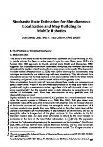
sidestep this issue by using only a single wireless card. Commercial systems usually use coarser COO techniques, thus removing the reliance on the absolute value of the RSS or uniform hardware, too. In [35] it was shown that normalization of the measurements to an appropriate scale goes a long way toward minimizing these differences and the impact they have on the underlying estimation algorithm. This normalization approach works only if each wireless card can be tested and calibrated before the online phase so as to determine the appropriate scale for normalization. Here, we present another possible approach that removes the need for normalization and calibration. By representing the RSS measured from each transmitter as a height at a specific location, one gets a height field reflecting the signal strength over the entire region. The peak of the height field would be at the transmitter where the signal is strongest. (Figure 7)
Figure 7: The radio map as a height field. Each color represents a different transmitter.
28
The RSS at locations other than at the transmitter will not be unique. Similar to a contour in topological terrain maps, RSS at locations other than the transmitter will be similar to some neighboring values, forming a closed loop on the surface of the height field. The agent may move in a few directions. Cardinal directions are clockwise and counter-clockwise along a contour, from a lower contour to a higher one and viceversa. Of course, other directions intermediate to these cardinal ones are possible. Since each transmitter has its own height field, a motion along a contour in one height field may be up a slope in another. This may aid in fingerprinting a location for the radio map technique. This phenomenon can be observed in Figure 7, which uses a small sample of the real experimental data from this research. Also noticeable in the figure is the relative heights (ranks) of each height field. For widely spaced transmitters, certain regions are dominated by a specific transmitter and their relative heights become important in identifying coarse regions. Furthermore, with these techniques, the number of APs has a more profound effect on the ability to resolve different positions. For example, with only one AP, the ranked height field method fails completely, since there is only one region (two, if the lack of any measurable signal is considered as a separate region). However, with each AP added, the number of distinct rankings increases at a factorial rate, corresponding to the number of permutations of the APs. It is also possible that the sizes of the regions are larger than the acceptable resolution of the algorithm. This would be counteracted by the motion model, which will account for motion within the region. In summary, when the radio map is considered as a collection of height fields, two alternative methods of measuring the RSS present themselves. The first method measures the gradient of the height field at each point, while the second considers the nominal ordering (the ranking) of the height fields relative to each other. These
29
methods are more robust predictors for location estimation than the raw RSS values they were derived from. It is necessary to use both gradients and ranked height fields since the gradient of the height field cannot be determined by instantaneous measurements alone and there may still be some ambiguity when relying solely on any one method alone. 4.3.7
Other Issues
In addition to the issues discussed above, Wi-Fi SLAM will need to perform global localization and requires an algorithm capable of representing arbitrary distributions. PFs were chosen for the final Wi-Fi SLAM algorithm because they can handle these requirements. There are also other aspects to Wi-Fi SLAM that are beyond the scope of this dissertation. These are considered hard problems in SLAM: recovery from catastrophic localization failure and operation in dynamic environments. However, PFs have been shown to be capable of recovery from catastrophic failures [50]. 4.3.8
Algorithm Details
An overview of the algorithm is presented in Figure 8. The algorithm starts with the initial particles at the upper-right corner of the figure. A detailed description of the algorithm’s implementation can be found in Appendix A. The particles will represent the possible locations of the agent. Each particle stores a list of positions of the agent, past and current. This differs from typical robotic SLAM, where the particle value is only the robot’s current pose. The historical position information, when combined with a common list of historical radio measurements, will provide enough information to construct a radio map of the environment for each particle. It is a concise way of storing the state of the environment and agent represented by the particle.
30
Particle filter
Initial particles
Site information
AP positions
Accessibility map
Human motion model
Update particle values
Simple radio model Radio measurements Radio model
Update particle weights
SLAM models
Figure 8: Algorithm block diagram. The particle values and weights are derived automatically from the map of the accessible areas of the building. The creation of the accessibility map is itself not currently part of the Wi-Fi SLAM algorithm and relies on manual intervention. Factoring in the presence of walls, hallways, rooms, voids, and other structures, the gray scale map will indicate the likely places a person may be. The next phases are the SLAM particle filter proper. Radio measurements are taken at regular intervals and, together with the models and other static information like the building layout and positions of the APs, are fed to these phases. These phases are repeated as long as there are new radio measurements and each step will yield a distribution of particles—the possible locations of the agent. As more measurements are made available, the user would be localized more precisely. 4.3.8.1
Prediction Phase
The prediction phase relies on the knowledge of the physical environment (building layout and positions of APs), the human motion model, and basic radio model to predict the likely next position of each particle, i.e., p(xk+1 |xk ) where xk and xk+1 31
are the particle position histories for the current and next step, respectively. Computationally, xk+1 is evaluated in a discrete grid instead of computing a continuous distribution. Further computational efficiency is obtained by evaluating xk+1 only within a small distance of xk since larger changes in position become increasingly improbable. This phase can be decomposed into four steps: 1. Use information about the physical structure of the building (walls, voids, etc) to determine accessibility and predict the possible new positions. 2. Use the human motion model (Section 4.3.5) to predict the likely next position. 3. Use information about the positions of the APs and a simple radio model to determine the likely direction and/or distance moved. 4. Combine the predictions from the earlier steps to form the final prediction. The accessibility step uses the static accessibility map derived at the start of the algorithm from the physical map of the building. For each particle, the algorithm will extract the corresponding region around the particle from this gray scale accessibility map. The basics of the motion model were described in Section 4.3.5. The model assumes a preference for a certain walking speed with the possibility of stopping (Figure 9), and that the user will prefer to walk in certain directions—mostly forwards, sometimes directly left or right, and rarely backwards (Figure 10). The walking speed is modeled by a normal distribution with parameters extracted from experimental data. For these particular experiments, there was no stopping, so this was not included in the model, but would be easy to add. Modeling the walking direction is somewhat more complicated. Each cardinal direction is modeled using a separate normal distribution, each with its own µ (centered at the particular cardinal direction) and σ parameters and weighted again to 32
describe the possibility of turns or backtracking. Again, parameters were extracted from experimental data. 0.6 0.5
Probability
0.4 0.3 0.2 0.1 0
0
0.25
0.5
0.75
1
1.25
1.5
Distance (multiple of average walking speed)
Figure 9: Example distribution for walking speed. As suggested in Section 4.3.4, the known positions of the APs, coupled with a simple radio model, can be used to assist in predicting the direction and distance of travel. The implemented algorithm uses a very basic radio model (signal strength decreases moving away from the AP and increases moving towards the AP) to predict the general direction of travel, but not the distance (Figure 11). The three previous steps will each yield a probability distribution of the next position of each particle. The distributions are combined equally to yield a final distribution. From the combined distribution, a position is picked randomly and us used as the new position for each particle. 4.3.8.2
Update Phase
The update phase in turn relies on the measured radio signals and a radio model (Section 6.2.3) to evaluate each particle’s likelihood. The model will express the probability of the measured signal given the model-computed signal at a given particle position, i.e., p(RSS measured |RSS model ). 33
0.01
Probability
0.008
0.006
0.004
0.002
0
0
90
180
270
360
◦
Direction ( clockwise from forward)
Figure 10: Example distribution for walking direction.
AP Equidistance from AP
Region of increasing RSS Region of particle motion
Particle position Region of decreasing RSS
Figure 11: Simple radio model to predict direction of travel.
34
The proposed radio model uses a normal distribution where measured radio signals further from the mean have a greater “spread” in their error distribution. The experimental results to justify this model are presented in Section 6.2.3. The final equations are
1
(RSS measured −RSS model )2 2σ 2 model
√ e σmodel 2π (RSS model −µ)2 1 2σ 2 = √ e− σ 2π
p(RSS measured |RSS model ) = σmodel
−
(10) (11)
It was determined experimentally (Section 6.2.3) that σ = 10 and µ = 30. However, if one uses gradients or ranked height fields as proposed in Section 4.3.6, the error model changes somewhat. Ranked height fields are resistant to environmental and sensor noise, while gradients proved more susceptible. For ranked height fields, the radio model will not model noise—only height fields that match exactly were considered. A suitable model for the radio gradients proved hard to determine since determining the gradients required multiple spatially separated radio measurements. The use of radio gradients may be investigated in future research.
35
CHAPTER 5 EXPERIMENTAL SETUP 5.1
Test Environment
The area being investigated is a section of the third floor of the Klaus Advanced Computing Building (Figure 12). The area chosen consists of primarily long, straight, narrow corridors. The measurements were done over several days. However, each measurement was assumed to be independent of the others and also independent of time. Each measurement was taken at approximately 1.35 m intervals (distance covered in 1 s at the author’s typical walking speed). When used in the algorithm, paths were constructed by selecting the appropriate measurements, simulating a human user walking along that path. Multiple paths could be assembled from the data since each point was measured several times. These paths were then used as input for the algorithm (Figure 13). The paths were chosen to test the performance of the algorithm when operating on long and short paths, turns, and slightly curved paths. All are closed loops so they could be repeated until the algorithm converges. There are hundreds of APs within detection range on the third floor. While this number may not be unusual for a research building, it is much higher than normal for most deployments. To reduce the volume of data and to eliminate transient or moving APs, only APs from the campus-wide GTwireless and FastPass network were used. These were filtered based on their broadcasted service set identifiers (SSIDs) in their beacons. It is important to bear in mind that the performance of the algorithm will depend highly on environmental conditions. A large empty hall with APs at each corner will be trivially easy to map compared to a maze of corridors with only a couple of APs. 36
37 Figure 12: Map of sections investigated.
(a)
(b)
(c)
(d)
Figure 13: Paths used for experiments.
38
The results presented in the subsequent chapter are specific to this environment.
5.2
Equipment Used
The equipment composed of an Apple Macbook laptop with Kismet wireless network monitoring software [29] and custom site-survey software. Multiple wireless network interfaces were used: the laptop’s built-in Atheros-based interface and an external USB RaLink-based dongle. Additional testing for radio gradients utilized another laptop with a built-in RaLink-based interface and a PRISM II-based PC Card with an external high-gain omnidirectional antenna. The Kismet software is capable of utilizing multiple wireless network interfaces monitoring simultaneously, channel hopping, raw packet logging, signal-strength logging, and interfacing with a GPS device via the gpsd [53] interface. Using GPS to aid in the site survey is out of the question—the motivation for this research is the inability to use GPS indoors and the low resolution of GPS. Instead of using a real GPS device, the custom Python software, Watchman, emulates one. Human input is required to indicate the physical location on a floor map (ground truth) and orientation (unused in current implementations of the algorithm). This data is then fed to Kismet to be logged together with the wireless network packets. This leverages the strengths of Kismet without unnecessary duplication of effort that would occur if the site survey software were developed from scratch. Kismet logs were processed by a Python program and stored in a MySQL database. The Wi-Fi SLAM algorithm was implemented using Python and NumPy/SciPy and drew on data from the database, with pre-processing for simulating user motion and calculating gradients. The locations of the APs were confirmed visually. The locations of APs on the third floor are indicated in Figure 14. The accessibility map, needed by the probabilistic algorithm, is shown overlaid on
39
40
Figure 14: Location of APs on the third floor of the Klaus Advanced Computing building.
the floor plan in Figure 15. Previous attempts in [35] used SVR for the estimation algorithm because of the need for interpolated locations between the original sample points. Training the SVR was a lengthy process and unsuitable for the new algorithm introduced here, which causes large changes in the training dataset each time new agent measurements are added. For the deterministic approach, the location estimation algorithm used is the simple k-NN. The probabilistic SLAM algorithm generates a probability distribution for the location of the agent and needs no further location estimation algorithm. For comparison, the same test data from the site survey is used with a k-NN location estimate serving as a control. The k-NN algorithm in both the deterministic approach and control used a simple Euclidean distance in the space of the radio map.
5.3
Particle Filter Implementation
The PF used in the Wi-Fi SLAM algorithm is a standard implementation. The main contribution of the research is not the PF but the models and use of RSS for SLAM. When the ESS of the particles falls below a threshold βN , the particles were resampled using a simple select with replacement algorithm.
5.4
Probabilistic Algorithm Parameters
The probabilistic algorithm has a number of parameters. Most of these were determined experimentally and discussed in Section 6.2. The initial particles were populated based on the accessibility map. The region being investigated is approximately 280 m2 . Assuming the particles are distributed are approximately 0.5 m apart, approximately 357 particles are required. The algorithm was run with 4000 particles to ensure adequate samples.
41
42 Figure 15: Gray scale accessibility map overlaid on floor plan.
5.5
Comparison Metrics
The basis for comparison is the accuracy of the location estimates and of the radio map. The new algorithm was compared with a method that utilizes a site survey in conjunction with a simple k-NN search to match the signal strengths. 5.5.1
k-NN Algorithm
The k-NN algorithm is a simple classifier and is one of the most basic machine learning algorithms available. Given a new object, one calculates the distance metric (typically Euclidean distance in the feature space) from that object to all other objects in the training set. From there, an arbitrary k neighbors are selected and the majority class of these k neighbors is the class of this new object. In terms of radio fingerprinting, one is given a set of radio measurements for the current position. One then finds the set of k measurements, from the measurements obtained during the site survey, that differ the least from the given measurements. Each of these k measurements will be at various positions. The majority position (or in the case of a tie, the average position) is the position of the new measurement. Using k-NN for radio fingerprinting typically limits the resolution of the estimates to the resolution of the site survey (the number of classes). It works well for small areas, but for larger areas with more radio measurements from the site survey and more APs, the distance calculations required become unwieldy. 5.5.2
Accuracy
Accuracy in localization systems, such as GPS, is often defined in terms of the uncertainty in the position. Often, it is assumed that the errors have a Gaussian distribution. Thus, it becomes possible to talk of an error ellipsoid that bounds the 95% (actually, two σ, or two standard deviations) confidence interval of the error region. Many systems will reduce this further to a single radius by taking the root-mean
43
square (RMS) of the horizontal and vertical components of the error region. The error distribution when using PFs is not necessarily Gaussian or elliptical, but can still be approximated by an error ellipse. Ninety-five percent of the particles should fall within this region. This was the primary metric for this research. The deterministic model discussed in the first half of this research makes no predictions as to its accuracy and will give the same estimate each time for the same data set. Instead of a 95% confidence interval, the absolute value of the error between the estimated position and ground truth was used. Where possible, the estimated radio map was compared qualitatively with the measured radio map. The measured radio map used measurements from the previous section but with values interpolated using inverse distance weighting (IDW). Though the radio map is of lesser importance than the actual location estimate, it gives insight to the errors of the location estimate that is derived from it. Briefly, IDW is a simple method for interpolating unevenly spaced 2D data [45]. The algorithm takes the general form of the function PN
u(x) = Pk=0 N
wk (x)uk
k=0 wk (x)
(12)
which basically states that the interpolated value u(x) is the weighted average wk (x) of all known points uk . In the simplest form, the weight is calculated using the inverse power of the distance of the interpolated point from the known point:
wk (x) =
1 d(x, xk )p
(13)
The distance function d is commonly the Euclidean distance and the value of p is commonly 2, corresponding to the inverse square law. There are many variations to the above formulae, especially for computing wk (x), to obtain more accurate interpolations, taking into account the areas of influence and
44
spatial distribution of the points. However, for our purposes, these basic formulae will suffice. When direct comparison of the RSS is used, it is important to note that the units are arbitrary since the wireless network interface itself reports in unspecified units. Most of the time, each unit is equivalent to 1 dB, and this assumption is used throughout this research. This assumption does not affect the results of this research since RSS units are only used relatively (there is no need for an absolute RSS measurement) or qualitatively.
45
CHAPTER 6 RESULTS AND DISCUSSION 6.1
Deterministic Modeling
Initial work on the problem focused on a deterministic model, mostly around obtaining a radio propagation model and then subsequently testing the algorithm against various environments. The transmit power and location of each AP were estimated using experimental data (Section 6.1), and the radio propagation model described in Section 4.3.4 was used to construct an approximate radio map of a circular area around each AP. Various radii for the approximated area were tested, ranging from 1 m to 4 m (approximately the size of a small room without any pillars or other obstructions). The agent trajectory was also estimated using a simple linear model. This deterministic model was tested in simple linear environments and in more complex planar environments. In the simple linear environments, the agent travels in a straight line approaching the transmitter, and then receding away from it. In the planar environments, the path of the agent may not intersect with the position of the transmitter and may also change direction. 6.1.1
Free-Space Model
The free-space model was described in Section 4.3.4, specifically Equation (9). Figure 16 shows how the free-space model deviates from the actual empirical measurements. White regions indicate where the free-space model falls below the empirical measurements, while black regions indicate the converse. In some cases, the deviation is only a few units, most notably in Figures 16d and 16e. Figure 16d exhibits a pattern similar to the two-ray propagation model,
46
16 0
12
20
8
40
4
60 0
80
−4
100
−8
120 140
−12 0
50
100
150
200 −16
(a) 00:15:C7:AB:39:40
25 0
20
20
15
40
10
60 80
5
100 0
120
−5
140 0
50
100
150
200 −10
(b) 00:15:C7:AB:04:21
Figure 16: Deviation of free-space models from empirical measurements by AP.
47
15 0 10
20
5
40 60
0
80 −5
100
−10
120 140 0
50
100
150
200
−15 −20
(c) 00:15:C7:AA:D6:61
8
0 20
4
40
0
60 −4
80 100
−8
120 −12
140 0
50
100
150
200
−16
(d) 00:15:C7:AA:E3:80
Figure 16: Deviation of free-space models from empirical measurements by AP.
48
8 0 4
20
0
40 60
−4
80
−8
100 −12
120
−16
140 0
50
100
150
200
−20
(e) 00:15:C7:AA:D5:30
Figure 16: Deviation of free-space models from empirical measurements by AP. which corresponds to a large open area in the floor plans. The other figures (Figures 16a to 16c and 16e) show APs that are placed in hallways, which exhibit the waveguide characteristics of the hallway where the signal is reinforced along the axis of the corridor but any paths branching off from the main axis have significantly lower RSS. While the form of the free-space model estimates coincides strongly with the measured values close to the transmitter, the actual estimates are offset by up to 27 units. This is indicated by regions of nearly uniform white in most of the figures. When used with the deterministic model, the free-space model consistently underestimates the distance between the transmitter and the agent. Moreover, the magnitude of this under-estimation varies from AP to AP. Thus, the inaccurate free-space approximation is one impediment to the deterministic model. However, when the free-space model is used to predict radio map gradients, one 49
will find a closer correlation between the free-space model and empirical measurements since there is a constant, albeit unknown, offset. Gradients were not used in the deterministic model, only in the probabilistic model. Their performance is detailed later in Section 6.2.1. 6.1.2
Deterministic Model Performance
Figure 17 shows the accuracy of the deterministic model as the radius of the free-space approximation region varies.
Figure 17: Accuracy of the deterministic model. The accuracy of the model decreases if the radius of the approximation region is too small or too large. The exact value for the best accuracy appears to be dependent on the particular characteristics of the region being mapped. Even when a “sweet spot” is found, the accuracy is poor, on the order of 5 m. 50
These results are for the deterministic model under ideal conditions. With more typical and less ideal conditions, the deterministic model tends to accumulate large errors and the map joining techniques fail. This proved far too limiting for practical use. The probabilistic approach discussed in the next chapter builds on the knowledge acquired from these problems and proved more successful.
6.2
Probabilistic Modeling
Most of the work for the initial phase was derived from the earlier deterministic model. The experimental data and radio model used here was the same as those used in the deterministic model. However, the range of the radio model was no longer confined to a small area but extended over the entire map. The physical map has been marked to indicate what areas are accessible. 6.2.1
Radio Map Gradients
Figure 18 shows the correlation between the gradients measured by two different wireless network cards—the built-in Macbook Atheros card and the external RaLink USB dongle. For small gradients, i.e., far away from the AP, there is a very good correlation. Closer to the transmitter where the gradients are steeper, there are greater variations in the gradients. This may be due to the specific antenna characteristics of the two wireless cards, making them susceptible to significant RSS variations when there is a strong direct signal present. Figure 19 shows the correlation between the gradients from the free-space model and the empirical measurements. The measured gradients show significant variance, mostly because of measurement noise. Smaller gradients (< 0.4) in both models are well correlated, and these are either positions further away from the AP or positions with less measurement noise.
51
Figure 18: Correlation of radio map gradients for different wireless network cards.
52
(a) 00:15:C7:AB:39:40
(b) 00:15:C7:AB:04:21
Figure 19: Correlation between free-space gradient approximations and empirical measurements. 53
(c) 00:15:C7:AA:D6:61
(d) 00:15:C7:AA:E3:80
Figure 19: Correlation between free-space gradient approximations and empirical measurements. 54
(e) 00:15:C7:AA:D5:30
Figure 19: Correlation between free-space gradient approximations and empirical measurements.
55
6.2.2
Motion Model
The layout of the building resulted in courses which were primarily straight lines with occasional turns, except in one part where the path was an arc. Coupled with the chosen test courses (Section 5.1), this means that there is no chance of backtracking and an estimated 1 in 10 chance of turning. After accounting for the 60◦ offset from north, virtually all paths are at right angles to each other. This means that there is only a small σ parameter for the motion model to handle the curved part of the building. 6.2.3
Radio Model
The radio model for the SLAM algorithm, based on the free-space model as described in Section 4.3.4, is derived in part from experimental data. The measured signal at a given location typically fluctuated around certain values due to sensor and environmental noise (Figure 20). So given a certain measured RSS at a particular location, the next measurement may be different even for the same position, constituting an error because of the sensor or a variation in the environment. Figure 21 shows the distribution of this error or variance. Each color represents a different measured RSS and the bars show the distribution of measurements with the error component factored in. It can be seen that the distributions can be approximated by a normal, but the actual parameters of the normal distribution vary somewhat depending on the original measured RSS. The parameters themselves seem to vary with the normal distribution. If σ 2 is varied according to a normal curve, we get a distribution as in Figure 22 when σ = 10 and µ = 30. Unfortunately, these values may be dependent on the particular test setup and there seems to be no easy way (rule of thumb, etc) to reduce the effort required in acquiring these parameters, short of a quick site survey.
56
(a) 00:15:C7:AB:39:40
(b) 00:15:C7:AB:04:21
Figure 20: Distribution of temporally super-sampled RSS. 57
(c) 00:15:C7:AA:D6:60
(d) 00:15:C7:AA:E3:80
Figure 20: Distribution of temporally super-sampled RSS. 58
(e) 00:15:C7:AA:D5:30
Figure 20: Distribution of temporally super-sampled RSS.
59
Figure 21: Distribution of temporally super-sampled RSS.
Figure 22: Distribution of temporally super-sampled RSS in the radio model. 60
6.2.4
Probabilistic Model Performance
The probabilistic model fared considerably better than the deterministic one. It was able to converge despite errors in the measurements and models. Figure 26 in Appendix B shows the algorithm tracking an agent along the straight hallway (the route in Figure 13a) after only about 4 minutes (230 iterations). This was done with no prior knowledge of the position of the agent or radio map, i.e., global localization. At this point, there was still considerable uncertainty over the agent’s exact position, as indicated by the spread of the distribution along the axis of the hallway. There was also some uncertainty when encountering the larger open space near the middle of the path. There were small but significant peaks in the particle distribution along the curved hallway that, while not being part of this particular route, were still part of the accessible area of the building. This “ghost” may be due to the fact that the access points being measured are near the center of the area pictured, and thus the straight hallway and curved hallway are approximately equidistant from it and are expected by the radio model to share similar radio measurements. Figure 27, also in Appendix B, shows the algorithm tracking the agent along part of the straight hallway, turning into the open area in the middle, and then again on the other stretch of straight hallway—an S-shaped course. These plots occur after more iterations than the previous example, so the localization was more accurate. At times, artifacts of the motion model can be seen, manifested as a two to four closely spaced peaks in the distribution. The algorithm remains confused about the central area of the building, which is a little more open than the narrow hallways. It is also likely that this region experiences nearly uniform RSS and is also similarly featureless when considering radio map regions. However, outside the region, the algorithm resumed accurate tracking of the agent.
61
6.2.5
Accuracy Improvement
Figure 23 shows how the accuracy of the algorithms improved over time as more radio measurements were accumulated for each of the paths in Figure 13 respectively. To put the accuracy in perspective, the furthest distance from the center of the test region was about 25 m, i.e., a “dumb” algorithm which predicts a position consistently in the center of the map will at worst be 25 m from the actual position. The proposed algorithms started with an accuracy of about 40 m because the starting points for the paths were near the corner of the map and the particles were spread over the entire map, giving an error of nearly the entire width of the map. Overall, the algorithms showed rapid improvement at the first lap of the course and subsequently more gradual trends. The cyclic peaks and troughs in the figures were caused mostly by the repeating nature of the test course. The algorithms typically reached their maximum accuracy after about four laps. The standard radio model, which did not utilize ranked radio maps or radio gradients (“no dir” in the figure), compares poorly with the algorithm using ranked radio maps and estimating direction from the radio measurements (“ranked dir” in the figure). The algorithm that estimated direction but did not utilize ranked radio maps (“dir”) has similar performance to the basic algorithm. It would seem that using the ranked radio maps filtered out the noise from the radio measurements and helped the PF settle on the correct particles. With ranked radio maps and direction estimation, the error radius settles in to a range of about 3 to 5 m. 6.2.6
Varying Number of APs
The radio fingerprinting approach relies on each location having a unique radio fingerprint. Section 4.3.6 states that the number of possible unique fingerprints is in turn dependent on the number of APs.
62
(a)
(b)
Figure 23: Accuracy of the algorithms over time. 63
(c)
(d)
Figure 23: Accuracy of the algorithms over time. 64
Figure 24 shows how the accuracy of the ranked radio map with direction estimation algorithm fared with various numbers of APs. There was a slight decrease in performance when the number of APs were reduced by one. When all but one of the APs were removed, the algorithm did not improve at all, since the number of regions dropped to one. The variation in accuracy increased as the number of available APs decreased.
Figure 24: Accuracy of the algorithm with different number of APs.
6.2.7
Comparison with Standard Approach
As mentioned in Section 5.5, the new algorithm was compared with a simple approach utilizing a radio map and the k-NN algorithm. Figure 25 shows the performance of the k-NN algorithm with different k. Tuning for the optimal parameters (k = 8), the simple approach yielded a mean error of 3.3 m. Given enough iterations, the SLAM algorithm compares favorably, at times performing slightly better or worse than the k-NN algorithm. 65
Figure 25: Accuracy of the k-NN algorithm with different k. The main benefit of the SLAM algorithm is the elimination of the site survey. Given the proper software tools, a user needs only a few minutes to an hour to mark the accessibility map and the locations of the APs. Doing the site survey, as required by the simple k-NN algorithm, will take at least a day and often more. The site survey for these experiments were done over the course of a few days.
66
CHAPTER 7 CONCLUSION The author started with the realization that current location estimation technologies are inefficient to set up—those using the radio fingerprinting method required an initial radio map that also needed significant time and effort to acquire. Eliminating the need for the initial radio map will make it easier to implement location estimation technologies. Thus, this research set about to eliminate the initial radio map, and the associated site survey, while still providing a reliable means of determining the user’s location. The initial deterministic approach was not sufficiently robust, and even under ideal conditions, had limited accuracy. This was due to the accumulation of errors and divergence of the maps from reality. This in turn was due to the deterministic algorithm selecting only the most probable choices at each step and ignoring other less likely choices that were actually correct. The subsequent probabilistic method, inspired by robotic SLAM, fared better because it modeled the uncertainty, only eliminating extremely improbable choices when necessary. The probabilistic approach, derived from robotic SLAM techniques, used some easily available information of the environment but did not require an initial radio map. There were several variants tested, each using slightly different radio models. The initial radio model for the SLAM updater, using the raw RSS measurements and not the radio height field-derived measurements, was complex and dependent on site-specific parameters. The dependence on site-specific parameters negates the potential benefits of SLAM compared to the normal site-survey approaches. In fact, it was too complex to model easily for the SLAM algorithm and performed poorly. The next versions of the radio model used a combination of ranked radio maps with direction estimates from the measured radio signals. The ranked radio maps proved
67
to be easier to model and more effective when used with the SLAM algorithm. The final algorithm was able to provide reasonably accurate location estimates, comparable to a simple k-NN algorithm, especially in the common scenario of narrow corridors. It did have problems in more open areas where the ranked radio maps provide little resolution. The algorithm’s performance was also limited by the number of APs, with significantly poorer performance when the number of APs was reduced.
7.1
Further Research
The ability of the algorithm to track agents in open indoor spaces was not tested—the experiments only considered narrow hallways with virtually one-dimensional motion. While this constitutes a large proportion of scenarios in typical real-world environments, it is also necessary to have an algorithm that is able to perform when the motion of the agent is not so limited. Initial tests (Section 6.2.4) indicate that open spaces caused the particle distribution to smear out and the algorithm to lose some accuracy. It is expected that the probabilistic method is more resistant to environmental variations, such as changes in room layout or large variations in building occupancy, than the deterministic method or even other contemporary methods utilizing the site survey. However, this could not be tested because of the intrinsic difficulty in controlling the test environment precisely. Future research may investigate this. However, it is important to note that robotic SLAM in highly dynamic environments has not been satisfactorily addressed by current literature either. Related to environmental variations is the variation of the agent’s position. The agent may move in a way unaccountable by the motion models, e.g., moving through regions that were supposedly inaccessible or separated by significant distance. This is known as catastrophic failure, and is another possibility that should be explored.
68
Finally, the ability to track and integrate information from multiple agents simultaneously was not investigated. There is some existing research on multi-robot SLAM [23, 51], and the techniques applied there could conceivably be extended to the particular environment of Wi-Fi SLAM.
69
APPENDIX A
ALGORITHM PSEUDOCODE
The following is a detailed pseudocode implementation of the Wi-Fi SLAM algorithm. The pseudocode is similar in syntax to the original Python/NumPy implementation used in this research, with some liberties taken for clarity. Particle filter implementation 1 # Initialize particles with initial state 2
particles = initial
3 # For each new set of RSS measurements coming in 4 for new_rss : 5
# Resample particles if necessary
6
if ess ( particles . weights ) < BETA * particles . count :
7
particles = resample ( particles )
8
# Actual particle filter step
9
particles . values = predictor ( particles , new_rss )
10
particles . weights = updater ( particles , new_rss )
11
# Normalize weights
12
particles . weights = normalize ( particles . weights )
13
# Increment step count
14
k += 1
15 16 # Calculate effective sample size ( ESS ) using the 17 # coefficient of variation . 18 def ess ( weights ) : 19
M = len ( weights )
70
20
cvtsq = (( M * weights - 1) ** 2) . sum () / M
21
esst = M / (1 + cvtsq )
22
return esst
23 24 # Select with replacement resampling . 25 def resample ( particles ) : 26
# Cumulative summation of weights
27
Q = particles . weights . cumsum ()
28
N = len ( weights )
29
# Generate N sorted random numbers , ending with 1
30
T = sorted ( random ( N ) . append (1) )
31
i = j = 0
32
# For each number in T ...
33
while i < N :
34
# ... chose it ( append its index to indices )
35
# if it is smaller than the corresponding Q
36
if T [ i ] < Q [ j ]:
37
indices . append ( j )
38
i += 1
39 40
else : j += 1
41
# Select the particles based on the indices
42
return particles [ indices ]
43 44 # Normalize all weights . 45 def normalize ( weights ) : 46
total = weights . sum ()
47
return weights / total
71
The particle filter is initialized with particle values derived from the accessibility map. It uses two functions, predict() and update(), which are part of the SLAM algorithm presented next. Wi-Fi SLAM prediction phase 1 # Prediction phase . Changes particle values . 2 def predictor ( particles , rss ) : 3
positions = particles . positions
4
# Append new signal to signal history
5
signals_history . append ( rss )
6
# Use accessibility to determine how user moved
7
access_positions = accessibility ( positions )
8
# Use motion model to determine how user moved
9
motion_positions = motion_model ( particles )
10
# Use radio model to determine how user moved
11
radio_positions = radio_model ( positions )
12
# Update particle positions
13
position_offsets = best_prediction ( access_positions , →
&
motion_positions , radio_positions )
14
new_positions = positions [ -1] + position_offsets
15
# Append new positions to original positions
16
new_positions = positions . append ( new_positions )
17
return new_positions
18 19
GRID_SIZE = ( PREDI CTION_ RADIUS * 2 / P R E D I C T I O N _ G R I D _ S I Z E )
20 21 # Returns an array for the distances offsets of the 22 # prediction grid .
72
23
DISTANCES2D = (( indices (( GRID_SIZE , GRID_SIZE ) ) * →
&
P R E D I C T I O N _ G R I D _ S I Z E ) - PR EDICTI ON_RAD IUS )
24 25 # Returns an array for the distances of the prediction grid . 26
DISTANCES1D = norm ( DISTANCES2D )
27 28 # Calculate new positions based on the accessibility bitmap . 29 def accessibility ( positions ) : 30
# Create a grid of sample points around each
31
# particle ’s current position
32
sampling_grid = positions [ -1] + DISTANCES2D
33
# Convert sampling grid to image coordinates
34
img_coords = longlat2image ( utm2longlat ( sampling_grid , →
zone ) )
35
# Get the probabilities for each grid position
36
s e l e c t e d _ p r o b a b i l i t i e s = ACCES SIBILI TY_MAP [ img_coords ]
37
return s e l e c t e d _ p r o b a b i l i t i e s
38 39 # Calculate new positions based on old positions and the 40 # motion model . 41 def motion_model ( particle ) : 42
# Calculate angle clockwise from " north "
43
angles = arctan ( DISTANCES2D .x , DISTANCES2D . y )
44
# Calculate current heading
45
headings = heading ( particle )
46
# Calculate angles of each grid square , relative to
47
# heading wrapping ranges to 0 1:
68
# Get last and second last position and
69
# calculate the direction vector
70
vectors = positions [ -1] - positions [ -2]
71
# Calculate the heading angle
72
headings = arctan ( vectors .x , vectors . y )
73
else :
74
# Calculate the angles , with an offset based on the
75
# building orientation
74
76
angles = ( range ( from -1 to 1 step 0.5) * PI + →
&
ORIENTATION )
77
# Generate particles . count integers in range [0 , 3]
78
random = random (4 , particles . count )
79
# Select the angles randomly from there
80
headings = choose ( random , angles )
81
return headings
82 83 # Calculate a normal distribution based on the angle 84 def angle_normal ( values , mean , multiplier ) : 85
angle_denom = (2 * ( ANGLE_VARIANCE ** 2) )
86
angle_a = 1 / ( ANGLE_VARIANCE * sqrt (2 * PI ) )
87
normal = angle_a * exp ( - square ( values - mean ) / ( & →
88
angle_denom ) )
return normal * multiplier
89 90 # Calculate a normal distribution based on the distance 91 def distance_normal () : 92
a = 1 / ( DISTAN CE_VAR IANCE * sqrt (2 * PI ) )
93
denom = (2 * ( DISTA NCE_VA RIANCE ** 2) )
94
normal = a * exp ( - square ( DISTANCES1D - STEP_SIZE ) / denom & →
95
)
return normal
96 97 # Calculate new positions based on old positions , new 98 # RSS , the radio model . 99 def radio_model ( positions ) : 100
# Last position of each particle
101
last_position = positions [ -1]
75
102
# Angle from each AP to each particle
103
deltas = ( last_position - GCM_AP_POSITIONS )
104
ap_angles = arctan ( deltas .x , deltas . y )
105
# Angle of regions for each AP for each particle
106
region_angles = ap_angles - PI / 2
107
# Increasing or decreasing RSS for each AP for each
108
# particle ?
109
last_signal = signals_history [ -2]
110
new_signal = signals_history [ -1]
111
signal_deltas = new_signal - last_signal
112
# Generate radio probabilities for each AP for each
113
# particle
114
for p a r t i c l e _ r e g i o n _ a n g l e s in region_angles :
115
for ( region_angle , signal_delta ) in ( & →
116
particle_region_angles , signal_deltas ) : particle_regions . append ( m a k e _ r a d i o _ p r o b a b i l i t i e s ( & →
117
region_angle , signal_delta ) )
regions . append ( particle_regions )
118
probabilities = regions . prod ()
119
return probabilities
120 121 # Create the appropriate radio probabilities for a given 122 # angle and signal 123 def m a k e _ r a d i o _ p r o b a b i l i t i e s ( angle , delta ) : 124
if delta == 0:
125
# Center only
126
grid = center_grid ()
127 128
else : # Some angle
76
129
if delta < 0:
130 131
tan = tan ( angle + PI ) else :
132
tan = tan ( angle )
133
# Generate rotated grid
134
grid = new_grid ()
135
for i in range ( len ( grid ) ) :
136
y = len ( grid ) / 2 - i
137
x = int ( y / tan )
138
j = x - len ( grid ) / 2
139
grid [i , j :] = RADIO_RATIO
140
return grid
141 142 # Generate grid for unchanging RSS 143 def center_grid () : 144
x = height * (1 - STOP_RADIUS ) * 0.5
145
y = width * (1 - STOP_RADIUS ) * 0.5
146
grid = new_grid ()
147
grid [ y :( len ( grid ) - y ) ,x :( len ( grid ) - x ) ] = RADIO_RATIO
148
return grid
149 150 # Calculate a weighted random position estimate for each 151 # particle . 152 def best_prediction ( particles , * predictions ) : 153
combined = combine ( predictions )
154
# Get best prediction for each particle
155
cumsum = combined . cumsum ()
156
r = random ( particles . count )
157
selected = ( cumsum < r ) . sum ()
77
158
selected_offsets = DISTANCES2D [ selection ]
159
return selected_offsets
160 161 # Combine the probability distributions together 162 def combine (* predictions ) : 163
# Combine individual predictions
164
for prediction in predictions :
165
prediction_sum = prediction . sum ()
166
# Check for particles with zero sums which
167
# will result in NaNs in the normalized values
168
nans = ( prediction_sum == 0)
169
normalized = prediction / prediction_sum
170
# Replace NaNs with zeroes
171
normalized [ nans ] = 0
172
product *= normalized
173
product_sum = product . sum ()
174
# Check for particles with zero sums ( NaNs )
175
nans = ( product_sum == 0)
176
product /= product_sum
177
# Set NaN particles to have no movement
178
product [ nans ] = 1
179
return product
Wi-Fi SLAM prediction update phase 1 # Update phase . Changes particle weights . 2 def updater ( particles , rss ) : 3
positions = particles . positions
4
weights = particles . weights
5
# Calculate radio map for each particle
78
6
for i , position in enumerate ( positions ) :
7
# Remove the first position , since it doesn ’t have a
8
# corresponding signal measurement , and the last
9
# position , since that ’s what we are testing
10
posi tion_l ess_on e = position [1: -1]
11
# Calculate radio map regions , again ignoring the
12
# latest signal measurements since that ’s what we are
13
# testing
14
radio_regions [ i ] = c a l c u l a t e _ r a d i o _ r e g i o n s ( & →
position_less_one , signals_history [: -1])
15
# Calculate ranking of latest signal
16
last_ranked = rss . argsort ()
17
# Calculate the weight of each particle based on the
18
# radio map regions and their similarity to the latest
19
# signals
20
diffs = ( radio_regions [ positions [ -1]] == last_ranked )
21
new_weights = weights / diffs . sum ()
22
# Normalize the weights
23
no rm al iz ed _w ei gh ts = ( new_weights / new_weights . sum () )
24
return n or ma li ze d_ we ig ht s
25 26 # Calculate the radio regions based on the nominal ordering 27 # of the RSS at each position . 28 def c a l c u l a t e _ r a d i o _ r e g i o n s ( positions , signals ) : 29
grid_positions = utm2grid ( positions , GRID_SIZE , GCM_BL )
30
# Generate radio map
31
radio_map = idw ( GRID_SIZE , GRID_SIZE , grid_positions , →
32
signals )
region_map = radio_map . argsort ()
79
&
33
return region_map
Remember that each particle’s value (particles.value) is a historical list of its past positions (particles.positions). The coordinates used are in longitude-latitude form. new_grid() creates a fixed-size grid of sample points, used to limit the algorithm to
a small but high-resolution area around each particle. This is an implementation optimization (Section 4.3.8.1). PREDICTION_RADIUS specifies the “radius” of the prediction area (actually the width and height of the square grid), and PREDICTION_GRID_SIZE specifies the resolution of the grid. In this implementation, both units are meters. FORWARDS_PROBABILITY, SIDEWAYS_PROBABILITY, and BACKWARDS_PROBABILITY and
the probabilities the user will head in a particular direction. STEP_SIZE is the average walking speed of the user. ANGLE_VARIANCE and DISTANCE_VARIANCE are the variances for the respective distributions. STOP_RATIO is the relative size of the probability distribution when the RSS does
not change, while RADIO_RATIO is the relative probabilities of the likely and unlikely directions of travel for the simple radio model. Finally, argsort(), which comes from NumPy, is the order of argument when arranged in increasing values. Supplementary functions 1 # Calculate the error radius of the given set of particles . 2 def ca lc ul at e_a cc ur ac y ( position , particles , percentile ) : 3
# Get most recent set of particle position estimates for
4
# each particle
5
pa rt ic le _p os it io ns = particles . positions [ -1]
6
u t m _ p a r t i c l e _ p o s i t i o n s = longlat2utm ( p art ic le _p os it io ns )
7
utm_position = longlat2utm ( position )
8
deltas = u t m _ p a r t i c l e _ p o s i t i o n s - utm_position
80
9
# Calculate the Euclidean distances for each particle
10
distances = norm ( deltas )
11
weights = particles . weights
12
# Sort distances and weights by distance
13
sorted_distances , sorted_weights = sorted (( distances , →
&
weights ) )
14
# Determine percentile index
15
target = sorted_weights . sum () * percentile
16
# Select only distances less than the target
17
indices = ( sorted_weights . cumsum () < target ) . sum ()
18
# Return selected accuracy radii
19
return sorted_distances [ indices ]
20 21 # Calculates a grid of RSS using IDW . 22
POWER = 2
23 def idw ( grid_height , grid_width , positions , radios ) : 24
# Calculate distances
25
deltas = indices (( grid_height , grid_width ) ) - positions
26
dists = norm ( deltas )
27
dp = power ( dists , - POWER )
28
total = dp . sum ()
29
# Calculate weights
30
weights = dp / total
31
# Fix singularities
32
count = len ( positions )
33
if count > 0:
34
nan_indices = ( positions == 0)
35
weights [ nan_indices ] = 1
36
values = sum ( weights * radios )
81
37
return values
38 39 # Calculate a grid of RSS using the inverse square law . 40 # Assumes each transmitter has unit power . 41 def free_space ( grid_height , grid_width , positions ) : 42
# Calculate distances
43
deltas = indices (( grid_height , grid_width ) ) - positions
44
distances = norm ( deltas )
45
weights = 1 / power ( distances , POWER )
46
# Fix singularities
47
weights [ positions ] = 1
48
return weights
82
APPENDIX B
TRACKING PERFORMANCE OF THE WI-FI SLAM ALGORITHM
The following figures illustrate a few iterations of the SLAM algorithm for various paths. The probability of the user being at a certain location is indicated by the color, varying from blue to yellow to red in increasing order of likelihood. The discussions associated with these figures are in Section 6.2.4.
83
230
231
232
233
234
235
Figure 26: Tracking a user moving along a straight hallway.
84
236
237
238
239
240
241
Figure 26: Tracking a user moving along a straight hallway.
85
242
243
244
245
246
247
Figure 26: Tracking a user moving along a straight hallway.
86
248
249
250
251
252
253
Figure 26: Tracking a user moving along a straight hallway.
87
254
255
256
257
258
259
Figure 26: Tracking a user moving along a straight hallway.
88
260
261
262
263
264
265
Figure 26: Tracking a user moving along a straight hallway.
89
266
267
268
269
270
271
Figure 26: Tracking a user moving along a straight hallway.
90
272
273
274
275
276
277
Figure 26: Tracking a user moving along a straight hallway.
91
278
279
280
281
282
283
Figure 26: Tracking a user moving along a straight hallway.
92
284
285
286
287
Figure 26: Tracking a user moving along a straight hallway.
93
431
432
433
434
435
436
Figure 27: Tracking a user moving along an S-shaped path.
94
437
438
439
440
441
442
Figure 27: Tracking a user moving along an S-shaped path.
95
443
444
445
446
447
448
Figure 27: Tracking a user moving along an S-shaped path.
96
449
450
451
452
453
454
Figure 27: Tracking a user moving along an S-shaped path.
97
455
456
457
458
459
460
Figure 27: Tracking a user moving along an S-shaped path.
98
461
462
463
464
465
466
Figure 27: Tracking a user moving along an S-shaped path.
99
467
468
469
470
471
472
Figure 27: Tracking a user moving along an S-shaped path.
100
473
474
Figure 27: Tracking a user moving along an S-shaped path.
101
REFERENCES
[1] G. D. Abowd, C. G. Atkeson, J. Hong, S. Long, R. Kooper, and M. Pinkerton, “Cyberguide: A mobile context-aware tour guide,” Wireless Networks, vol. 3, no. 5, pp. 421–433, October 1997. [2] AeroScout, “AeroScout,” Website, August 2004. [Online]. Available: http: //www.aeroscout.com/ [3] AirDefense, “AirDefense,” Website, August 2004. [Online]. Available: http: //www.airdefense.net/ [4] arkasha and bobzilla, “WiGLE - wireless geographic logging engine - plotting WiFi on maps,” Website. [Online]. Available: http://www.wigle.net/ [5] P. Bahl and V. N. Padmanabhan, “RADAR: An in-building RF-based user location and tracking system,” in Proceedings of 19th IEEE Conference on Computer Communication, vol. 2. IEEE, March 2000, pp. 775–784. [6] R. Battiti, M. Brunato, and A. Villani, “Statistical learning theory for location fingerprinting in wireless LANs,” Online document, University of Trento, Tech. Rep. DIT-02-086, October 2002. [Online]. Available: http://eprints.biblio.unitn.it/archive/00000238/01/86.pdf [7] M. Berna, B. Sellner, B. Lisien, S. Thrun, G. Gordon, and F. Pfenning, “A learning algorithm for localizing people based on wireless signal strength that uses labeled and unlabeled data,” 2003. [Online]. Available: http://www-2.cs.cmu.edu/∼fp/papers/wireless03.pdf [8] P. J. Brown, “The stick-e document: A framework for creating context-aware applications,” in Proceedings Electronic Publishing, January 1996, pp. 259–272. [9] M. Brunato and C. K. Kall´o, “Transparent location fingerprinting for wireless services,” in Proceedings of First Mediterranean Ad Hoc Networking Workshop, 2002. ˇ [10] S. Capkun, M. Hamdi, and J.-P. Hubaux, “GPS-free positioning in mobile adhoc networks,” in Proceedings of 34th Annual Hawaii International Conference on System Sciences. IEEE, January 2001. [11] P. Castro, P. Chiu, T. Kremenek, and R. R. Muntz, “A probabilistic room location service for wireless networked environments,” in Proceedings of 3rd International Conference on Ubiquitous Computing. ACM, 2001, pp. 18–34.
102
[12] N. Cristianini and J. Shawe-Taylor, An Introduction to Support Vector Machines and other kernel-based learning methods. Cambridge University Press, 2000. [13] D. E. Denning and P. F. MacDoran, “Location-based authentication: Grounding cyberspace for better security,” in Computer Fraud & Security. Elsevier Science Ltd., 1996. [14] Ekahau, “Ekahau,” //www.ekahau.com/
Website,
August 2004. [Online]. Available:
http:
[15] FCC, “FCC adopts rules to implement Enhanced 911 for wireless services,” Online document. [Online]. Available: http://www.fcc.gov/Bureaus/Wireless/ News Releases/1996/nrwl6026.txt [16] S. Ganu, A. S. Krishnakumar, and P. Krishnan, “Infrastructure-based location estimation in WLAN networks,” in Proceedings of IEEE Wireless Communications and Networking Conference. IEEE, 2004. [17] Google, “Google latitude,” Website. [Online]. Available: http://www.google. com/latitude/intro.html [18] A. G¨ unther and C. Hoene, “Measuring round trip times to determine the distance between WLAN nodes,” Telecommunication Networking Group, Technical University of Berlin, TKN-04-16, December 2004. [19] Y. Gwon, R. Jain, and T. Kawahara, “Robust indoor location estimation of stationary and mobile users,” in Proceedings of 23rd IEEE Conference on Computer Communication. IEEE, 2004. [20] A. Hatami and K. Pahlavan, “In-building intruder detection for WLAN access,” in Proceedings of Position Location and Navigation Symposium, 2004, pp. 592– 597. [21] P. Heckbert, “Bilinear Coons patch image warping,” in Graphics Gems IV, P. Heckbert, Ed. Boston: Academic Press, 1994, pp. 438–446, color plate VIII.2. [22] J. Hightower, B. Brumitt, and G. Borriello, “The location stack: A layered model for location in ubiquitous computing,” in Proceedings of 4th IEEE Workshop of Mobile Computing Systems & Applications. IEEE, June 2002, pp. 22–28. [23] A. Howard, “Multi-robot simultaneous localization and mapping using particle filters,” International Journal of Robotics Research, vol. 25, no. 12, pp. 1243– 1256, 2006. [Online]. Available: http://ijr.sagepub.com/cgi/content/abstract/ 25/12/1243 [24] IEEE, “ANSI/IEEE standard IEEE 802.11,” Online document, 1999. [Online]. Available: http://standards.ieee.org/getieee802/download/802.11-1999.pdf
103
[25] Intel Research Seattle, “Welcome to the Place Lab homepage,” Website, 2007. [Online]. Available: http://www.placelab.org/ [26] K. Kaemarungsi and P. Krishnamurthy, “Modeling of indoor positioning systems based on location fingerprinting,” in Proceedings of 23rd IEEE Conference on Computer Communication. IEEE, 2004. [27] E. D. Kaplan, Understanding GPS: Principles and Applications. Artech House, 1996. [28] A. Kehagias, J. Djugash, and S. Singh, “Range-only SLAM with interpolated range data,” Robotics Institute, Carnegie Mellon University, Pittsburgh, PA, Tech. Rep. CMU-RI-TR-06-26, May 2006. [29] M. Kershaw, “Kismet,” Website, 2007. [Online]. Available: kismetwireless.net/
http://www.
[30] J. Krumm and J. Platt, “Minimizing calibration effort for an indoor 802.11 device location measurement system,” in Neural Information Processing Systems, 2003. [31] D. Kurth, “Range-only robot localization and SLAM with radio,” Robotics Institute, Carnegie Mellon University, Tech. Rep. CMU-RI-TR-04-29, 2004. [Online]. Available: http://www.frc.ri.cmu.edu/projects/emergencyresponse/ parrotData/docs/kurth thesis.pdf [32] A. M. Ladd, K. E. Bekris, G. Marceau, A. Rudys, L. E. Kavraki, and D. S. Wallach, “Robotics-based location sensing using wireless Ethernet,” in Proceedings of ACM Annual Conference on Mobile Computing and Networking. ACM, September 2002, pp. 227–238. [Online]. Available: citeseer.ist.psu.edu/ article/ladd02roboticsbased.html [33] J. Leonard and H. Durrant-Whyte, “Mobile robot localization by tracking geometric beacons,” IEEE Transactions on Robotics and Automation, vol. 7, no. 3, pp. 376–382, 1991. [34] S. Li, G. Zhao, and L. Liao, “User location service over an 802.11 ad-hoc network,” December 2002. [Online]. Available: http://www.cs.washington.edu/ homes/liaolin/Courses/networks02.pdf [35] Y.-X. Lim, “Secure geo-location for wireless indoor networks,” Master’s thesis, Georgia Institute of Technology, May 2006. [36] Y.-X. Lim, T. Schmoyer, J. Levine, and H. Owen, “Wireless intrusion detection and response,” in Proceedings of the 4th Annual Information Assurance Workshop, June 2003. [37] A. Neskovic, N. Nescovic, and G. Paunovic, “Modern approaches in modeling of mobile radio systems propgation environments,” Communications Surveys, vol. 3, no. 3, pp. 1–12, 2000. 104
[38] D. Niculescu and B. Nath, “Ad hoc positioning system (APS) using AOA,” in Proceedings of 24th IEEE Conference on Computer Communication, vol. 3. IEEE, March 2003. [39] K. Pahlavan, X. Li, and J.-P. M¨akel¨a, “Indoor geolocation science and technology,” IEEE Communications Magazine, vol. 40, no. 2, pp. 112–118, February 2002. [40] M. Parciga, “Herecast,” Website, August 2005. [Online]. Available: //www.herecast.com/
http:
[41] N. Patwari, A. O. Hero III, M. Perkins, N. S. Correal, and R. J. O’Dea, “Relative location estimation in wireless sensor networks,” Transactions on Signal Processing, vol. 51, no. 8, August 2003. [42] H. Ralston, “Energy-speed relation and optimal speed during level walking,” European Journal of Applied Physiology, vol. 17, no. 4, pp. 277–283, October 1958. [Online]. Available: http://dx.doi.org/10.1007/BF00698754 [43] I. Rhee, M. Shin, S. Hong, K. Lee, and S. Chong, “On the levy-walk nature of human mobility: Do humans walk like monkeys?” in Proceedings of 27th IEEE Conference on Computer Communication, 2008. [44] T. Schmoyer, Y.-X. Lim, and H. Owen, “Wireless intrusion detection and response: A case study using the classic man-in-the-middle attack,” in Proceedings of Wireless Communications and Networking Conference, 2004. [45] D. Shepard, “A two-dimensional interpolation function for irregularly-spaced data,” in Proceedings of 23rd ACM National Conference. New York, NY, USA: ACM, 1968, pp. 517–524. [46] Skyhook Wireless, “Skyhook wireless,” Website, August 2004. [Online]. Available: http://www.skyhookwireless.com/ [47] J. Small, A. Smailagic, and D. P. Siewiorek, “Determining user location for context aware computing through the use of a wireless LAN infrastructure,” December 2000. [Online]. Available: http://www-2.cs.cmu.edu/∼aura/docdir/ small00.pdf [48] J. R. Spletzer, “A new approach to range-only SLAM for wireless sensor networks,” Lehigh University, Tech. Rep. LU-CSE-04-008, 2004. [Online]. Available: http://www3.lehigh.edu/images/userImages/jgs2/Page 3813/LU-CSE-04-008.pdf [49] N. Sundaram and P. Ramanathan, “Connectivity based location estimation scheme for wireless ad hoc networks,” in Proceedings of Global Telecommunications Conference, vol. 1. IEEE, 2002, pp. 143–147.
105
[50] S. Thrun, D. Fox, W. Burgard, and F. Dellaert, “Robust Monte Carlo localization for mobile robots,” Artificial Intelligence, vol. 128, no. 1-2, pp. 99–141, 2000. [51] S. Thrun and Y. Liu, “Multi-robot SLAM with sparse extended information filers,” in Robotics Research, ser. Springer Tracts in Advanced Robotics, vol. 15. Springer Berlin/Heidelberg, 2005. [Online]. Available: http: //robots.stanford.edu/papers/Thrun03e.pdf [52] T. Tonteri, “A statistical modeling approach to location estimation,” Master’s thesis, University of Helsinki, May 2001. [53] R. Treffkorn, “GPSd — put your GPS on the net,” Website, June 2007. [Online]. Available: http://gpsd.berlios.de/ [54] J. Yin, Q. Yang, and L. Ni, “Adaptive temporal radio maps for indoor location estimation,” in Proceedings of 3rd IEEE International Conference on Pervasive Computing and Communications. IEEE, 2005. [55] M. A. Youssef and A. K. Agrawala, “Small-scale compensation for WLAN location determination systems,” in Proceeedings of Wireless Communications and Networking Conference. IEEE, March 2003. [56] ——, “Continuous space estimation for WLAN location determination systems,” in Proceedings of International Conference on Computer Communications and Networks, no. 13. IEEE, October 2004. [57] G. V. Z´aruba, M. Huber, and F. A. Kamangar, “Monte Carlo sampling based in-home location tracking with minimal RF infrastructure requirements,” in Proceedings of Global Telecommunications Conference, vol. 6. IEEE, 2004, pp. 3624–3629.
106