Efficiently Decodable and Searchable ∗ Natural Language Adaptive Compression Nieves R. Brisaboa
Antonio Farina ˜
Gonzalo Navarro
Jose´ R. Parama´
Fac. de Informatica, ´ Univ. da Coruna, ˜ A Coruna, ˜ Spain.
Fac. de Informatica, ´ Univ. da Coruna, ˜ A Coruna, ˜ Spain.
Dept. of Computer Science, Univ. of Chile, Santiago, Chile.
Fac. de Informatica, ´ Univ. da Coruna, ˜ A Coruna, ˜ Spain.
[email protected]
[email protected]
[email protected]
[email protected]
ABSTRACT We address the problem of adaptive compression of natural language text, focusing on the case where low bandwidth is available and the receiver has little processing power, as in mobile applications. Our technique achieves compression ratios around 32% and requires very little effort from the receiver. This tradeoff, not previously achieved with alternative techniques, is obtained by breaking the usual symmetry between sender and receiver present in statistical adaptive compression. Moreover, we show that our technique can be adapted to avoid decompression at all in cases where the receiver only wants to detect the presence of some keywords in the document, which is useful in scenarios such as selective dissemination of information, news clipping, alert systems, text categorization, and clustering. We show that, thanks to the same asymmetry, the receiver can search the compressed text much faster than the plain text. This was previously achieved only in semistatic compression scenarios.
1.
INTRODUCTION
Text compression [2] permits representing a document using less space. This is useful not only to save disk space, but more importantly, to save disk transfer and network transmission time. In recent years, compression techniques especially designed for natural language texts have not only proven extremely effective (with compression ratios around 25%-30%), but also permitted searching the compressed text much faster (up to 8 times) than the original text [20, 9, 10]. The integration of compression and indexing techniques [21, 17, 25] opened the door to compressed text databases, where texts and indexes are manipulated directly in compressed form, and both time and space are simultaneously saved. ∗Partially supported by CYTED VII.19 RIBIDI Project. Also funded in part (for the Spanish group) by MCyT (PGE and FEDER) grant(TIC2003-06593) and (for the third author) by Millennium Nucleus Center for Web Research, Grant (P01-029-F), Mideplan, Chile.
Permission to make digital or hard copies of all or part of this work for personal or classroom use is granted without fee provided that copies are not made or distributed for profit or commercial advantage and that copies bear this notice and the full citation on the first page. To copy otherwise, to republish, to post on servers or to redistribute to lists, requires prior specific permission and/or a fee. Copyright 200X ACM X-XXXXX-XX-X/XX/XX ...$5.00.
The key to the success of natural language text compression is the use of a word-based model [15], so that the text is regarded as a sequence of words. This poses the overhead of managing a large source alphabet, but in large text collections the vocabulary size is relatively insignificant because of Heaps Law [12]. Since the distribution of words is rather biased, following a Zipf Law [22, 1], the sequence of words is highly compressible with a zero-order encoder such as Huffman code [14]. In order to be searchable, semistatic models have been used in compressed text databases, to ensure that the codeword assigned to a word does not change across the text. Thus, a pattern can be compressed and directly searched for in the compressed text without decompressing it. This is also essential to permit local decompression of text passages in order to present them to the final users. Different searchable, word-based, semistatic statistical compressors with different merits have been used, such as bit-oriented Huffman [20], byte-oriented Huffman and variants [10], and the more recent End-Tagged Dense Codes and (s, c)-Dense Codes [6, 4]. As explained, documents are decompressed only in order to present them. A problem not addressed with the current schemes is how to transmit individual documents in compressed form. This is very interesting when the text server must transfer the documents through a low-bandwidth network. Note that it is not feasible to directly transfer the document as it is compressed in the database, because the receiver does not know the semistatic model used by the sender (which includes the vocabulary of the whole collection), and the overhead of transmitting it would be prohibitive, as the collection vocabulary is large when compared to the size of individual documents. Adaptive or dynamic,compression methods do not need to transmit the model because the receiver can learn it as it receives the compressed text. They have the additional advantage over semistatic methods that the sender does not need to perform a first pass over the text to build the model, but it can start the compression and transmission immediately, while the receiver can start reception and decompression simultaneously. A way to transmit individual documents in a compressed text database scenario is that the server uncompresses them and then recompresses them with an adaptive method. Note that transmitting an individual document with an adaptive scheme might not be very effective because there is not much time to converge to a good model. This is especially valid in word-based models because even the local
vocabulary of the document (which is transmitted as new symbols as they appear) is relatively large for small documents, again by Heaps Law [12]. Yet, this works well when the client establishes a longer session with the text server and several documents are transmitted along time. This can be precisely the case of a user session in a compressed text database, when browsing a digital library or a Web site, or in a chat or email service. There are some scenarios where the receiver can be interested not in uncompressing the arriving text, but just in searching it for some specific words, for classification or retrieval purposes. This has applications in selective dissemination of information, news clipping, altert systems and others. In all those cases, documents gathered from different sources are received and pointed out to users when keywords are found that denote topics of interest. Another application is text categorization and clustering, where documents gathered from text servers are classified according to the presence of certain keywords, without need to ever having the text at the categorization machine. For example, a language classification system might look for a small set of common words of each language and use it to classify the incoming compressed text, forwarding it to a specific directory or computer depending of its language, to be indexed, stored, or even automatically translated. Therefore it would be useful to have a dynamic compression method with direct search capabilities, that is, permitting direct search of the compressed text without decompressing it. However, direct search of text compressed with an adaptive technique is far more difficult than with a semistatic technique, as a given pattern looks different throughout the compressed document. Although there exist direct search techniques for adaptive compression that are more efficient than uncompressing and searching [19], semistatic compression permits much faster searching, faster than just searching the uncompressed text (without counting the time to uncompress) [10]. The best known adaptive compression methods are the Ziv-Lempel family [23, 24] and dynamic arithmetic coding [16]. The former obtains reasonable but not spectacular compression ratios (around 40%). The latter compresses much better (around 25%), but it requires significant computational effort both from the sender and from the receiver. This is especially unfortunate in cases where the receiver has limited computational power, such as in mobile applications. This symmetry in the sender and receiver efforts is at the essence of statistical adaptive compression, as both have to update their models in synchronization. It is also central to the difficulty of direct searching text compressed with adaptive methods. In [5, 11], adaptive versions of both word-based byteoriented Huffman and End-Tagged Dense Code (ETDC) were presented. The latter turns out to be especially interesting, achieving around 30% compression ratio and a compression speed close to the fastest Ziv-Lempel compressors (which achieve only 40% compression ratio) and 2.5 times faster than word-based arithmetic coding. Decompression is 3.5 times faster than with word-based arithmetic coding, but still twice as slow as the Ziv-Lempel compressors. In this paper we improve the existing results on wordbased adaptive compression, focusing on reducing the effort of the receiver in order to either uncompress or search the compressed text. We present a variant of the previous Dy-
namic End Tagged Dense Code (DETDC), that we call Dynamic Lightweight End Tagged Dense Code (DLETDC). DLETDC has almost exactly the same compression ratio of ETDC and DETDC, but it requires much less processing effort from the receiver than DETDC. As a result, decompression time is now similar to that of Ziv-Lempel methods in short files and better in longer files. The key idea is to relief the receiver from maintaining the model as it receives the text, but letting the sender inform of the changes when necessary. For this to be useful, we designed DLETDC so as to maintain its compression ratio while minimizing the required updates to the model. This breaks the usual symmetric model of statistical adaptive compression. Our second contribution focuses on the case where the receiver does not need to recover the original text, but just to detect the presence of some keywords in it. We show how DLETDC compressed text can be searched without decompressing it. The search algorithm is even lighter than the uncompression algorithm. It needs very little memory and can perform efficient Boyer-Moore-type searching on the compressed text. We show that searching the compressed text for a set of keywords is much faster (up to 5 times) over our compressed text than over the uncompressed text. This breaks another long-standing assumption that states that only semistatic models permit efficient Boyer-Moore searching on the compressed text. In particular, this is the first adaptive compression scheme that permits searching the compressed text faster than the uncompressed text.
2. RELATED WORK 2.1 Word-based Huffman codes Huffman code is the optimal (shortest total length) statistical prefix code for a given text. However traditional implementations of the Huffman code are character-based, (they use characters as source symbols) and therefore they obtain poor (around 65%) compression ratios. The brilliant wordbased approach, proposed by Moffat [15], yields much better compression ratios, close to 25%, using a binary target alphabet, that is, each word in the source text is encoded as a sequence of bits. In [10] two byte oriented word-based Huffman codes were proposed, called Plain Huffman and Tagged Huffman respectively. Plain Huffman does not modify the basic Huffman code except by using bytes as the symbols of the target alphabet. It obtains compression ratios close to 30% on natural language text. The loss in compression is due to the use of bytes instead of bits as in [15]. In exchange, decompression and searching are much faster with Plain Huffman code because no bit manipulations are necessary. In Tagged Huffman [10], the first bit of each byte is reserved to flag whether the byte is the first of its codeword. Hence, only 7 bits of each byte are used for the Huffman code. Note that the use of a Huffman code over the remaining 7 bits is mandatory, as the flag is not useful by itself to make the code a prefix code. While searching Plain Huffman compressed text requires inspecting all its bytes from the beginning, the tag bit in Tagged Huffman permits BoyerMoore-type searching (that is, skipping bytes) [3] by simply compressing the pattern and then running the string matching algorithm. On Plain Huffman this does not work, as the pattern could occur in the text not aligned to any codeword [10]. The problem is that the concatenation of two code-
words may contain the codeword of another source symbol. This cannot happen in Tagged Huffman code thanks to the tag bit that distinguishes initial codeword bytes. On the other hand, Tagged Huffman code pays a price in terms of compression performance of approximately 11%, as it stores full bytes but uses only 7 bits for coding.
2.2 End Tagged Dense Codes End-Tagged Dense Code (ETDC) [6] is obtained by a seemingly dull change to the Tagged Huffman Code [10]. Instead of using a flag bit to signal the beginning of a codeword, the end of a codeword is signaled. That is, the highest bit of any codeword byte is 0 except for the last byte, where it is 1. This change has surprising consequences. Now the flag bit is enough to ensure that the code is a prefix code regardless of the contents of the other 7 bits of each byte. To see this, consider two codewords X and Y , being X shorter than Y (|X| < |Y |). X cannot be a prefix of Y because the last byte of X has its flag bit in 1, while the |X|-th byte of Y has its flag bit in 0. Thanks to this change, there is no need at all to use Huffman coding in order to maintain a prefix code. Therefore, all possible combinations of bits can be used over the remaining 7 bits of each byte, producing a dense encoding. This yields a better compression ratio than Tagged Huffman while keeping all its good searching and decompression capabilities. On the other hand, ETDC is easier to build and faster in both compression and decompression. In general, ETDC can be defined over symbols of b bits, although in this paper we focus on the byte-oriented version where b = 8. ETDC is formally defined as follows. Definition 1. Given source symbols with decreasing probabilities {pi }0≤i |Cj |. As we explain later, sj is the first word (at the top) in the group of words with the same frequency of si . Thus, DLETDC needs two special codewords, Cnew−Symbol and Cswap . Cnew−Symbol works as was explained for DETDC. Cswap specifies that the receiver should swap the words at the positions pointed by the two codewords that follow Cswap . That is, Cswap ,Ci ,Cj indicates that now si is represented by Cj , and sj by Ci . This is implemented by a simple swap of words at positions i and j of the vocabulary array in the receiver. The key idea of this approach is that now there is no correspondence between the word rank (position in the frequencysorted vocabulary of the sender) and its codeword, because words change their positions without changing their codewords. That is, changes in the rank of a word do not produce changes in its codeword except when the codeword must be shorter. Therefore, the sender must maintain an explicit words-codewords mapping, and use it to encode words. Codewords Cnew−Symbol and Cswap can be the first two unused codewords, or the two last codewords of n bytes, being n the codeword size of the last word in the vocabulary
Example 1. Figure 1 shows an example of the process carried out by the sender. Assume that, after compressing a portion of a text, word "the" is in the 127th position of the sorted vocabulary, "is" is at the 128th position, and "beautiful" is at the 129th position, all of them with frequency 19. Assume that the text to be compressed next is "the rose rose beautiful beautiful". After reading "the", the compressor checks that "the" is already in the vocabulary and increases its frequency by 1. Next, the compressor recomputes the sorted vocabulary. We assume that "the" remains at position 127. Then the compressor sends codeword C127 . The next word ("rose") is not in the vocabulary, thus the compressor adds it to the vocabulary at the last position (last = 130) and gives it the codeword corresponding to that position, C130 . In order to inform the receiver of this addition, the encoder sends Cnew−Symbol and the word "rose" in plain form. The first occurrence of "beautiful" increases its frequency to 20 and then, after the reorganization, "beautiful" is relocated at the 128th position, swapping it with "is". However, since C128 (the codeword representing "is") and C129 (the one that represents "beautiful") have the same size (two bytes), the encoder continues using C128 to represent "is" and C129 to represent "beautiful". The next occurrence of "beautiful" places it at the 127th position, which has an associated codeword of one byte. Then, since in this case C127 and C129 have different sizes, the encoder swaps those codewords, associating "the" with C129 and "beautiful" with C127 . Hence, the receiver should be informed of this change. The encoder sends the tuple Cswap , C129 , C127 : Cswap warns the receiver to expect two codewords that should be exchanged. In addition, the receiver also understands that the second codeword (after the swap) is the word that was actually read. 2
words groups
DYNAMIC LIGHTWEIGHT END TAGGED DENSE CODE
word posInVoc freq codeword
C 3 2 C3
A 2 2 C1
1
2
3
4
5
top
0
1
2 2
1 3
4
posInHT
7 1
5 2
3 3
4
5
B 1 3 C2 6
7
8
last = 4
ABABBCCC hash table
3.
in a specific moment of the process. Another possibility is to give them fixed values across the whole process. In our implementation, we used the last two codewords of 3 bytes, since all our experimental corpora can be encoded with codewords of 3 bytes or less. These decisions involve a tradeoff between compression ratio on one hand and decompression and scanning speed on the other, as we will explain later.
words groups
the sender and the receiver are in charge of maintaining the sorted vocabulary, carrying out two symmetric processes. That is, a word position in the ranked vocabulary is the only necessary data to encode a word, because the mathematical correspondence rank-codeword explained in section 2.2 is used to compute the words-codewords mapping. Details can be found in [5].
word
C 2 3 C3
posInVoc freq codeword
A 3 2 C1
1
2
3
4
5
top
0
1
3 2
1 3
4
posInHT
7 1
3 2
5 3
4
5
B 1 3 C2 6
7
8
last = 4
Figure 2: Structures of the sender.
Word parsed In vocabulary?
………..
129
19 beautiful
130
--
is
19
19 beautiful
--
is
19
19 beautiful 1
Pos
C127 128 beautiful20 C129 129 is 19 C128 130 rose 2 C130
Figure 1: Example of compression.
The sender maintains a hash table that permits fast searching for any source word si to obtain its current position p in the rank, as well as its current frequency and codeword. Essentially, we must be able to identify groups of words with the same frequency, and be able of fast promoting a word to the next group when its frequency increases. Sender ( ) (1) Initialize vocabulary structures, last ← 0; (2) for i ∈ 1 . . . m do (3) readsi from the text; (4) p ← hash(si ); (5) if word(p) = empty (word not in vocabulary) then (6) send Cnew−Symbol ; (7) send si in plain form; (8) word[p] ← si ; (9) posInV oc[p] ← last; (10) f req[p] ← 1; (11) codeword[p] ← Clast ; (12) posInHT [last] ← p; (13) last ← last + 1; (14) else (15) Ci ← codeword[p]; (16) j ← top[f req[p]]; (17) If size(codeword[posInHT [j]]) < size(Ci ) then (18) send {Cswap , Ci , codeword[posInHT [j]]}; (19) swap(codeword[p], codeword[posInHT [j]]); (20) else (21) send Ci ; (22) swap(posInHT [posInV oc[p]], posInHT [j]); (23) swap(posInV oc[p], posInV oc[posInHT [j]]); (24) top[f req[p]] ← top[f req[p]] + 1; (25) f req[p] ← f req[p] + 1;
Figure 3: Sender processes in DLETDC The data structures used by the sender and their functionality are shown in Figure 2. The hash table of words keeps in word the source word, in posInVoc the position of the word in the rank, in freq its frequency and in codeword its codeword. In the vocabulary array (posInHT) words are not explicitly represented, but a pointer to the word slot in the hash table is stored. Finally the array top stores, for each possible frequency, the position in the rank (that is, in array posInHT) of the first word with that frequency. That is, top[13] = 7 means that the word in position 7 has frequency 13, but the word in position 6 has a higher frequency. If no words of frequency f exist, then top[f ] = −1. A variable last storing the first unused position of the vocabulary array is also needed. When the sender reads a word si , it uses the hash function to obtain its position p in the hash table, so that hash(si ) = p and therefore word[p] = si . The position of si in the rank is obtained as i = posInV oc[p] and its codeword as Ci = codeword[p]. In the same way f = f req[p]. Now,
Code
the 20
……
……
……
……
C130
Code
the 20 C127 127
19 C128 128 is C128 19 129 C129 beautiful C129 2 130 rose C130 130 rose C130
C128 128 C129 129
……
C128 128 C129 129 C130 130
Code Pos
the 20 C127 127
Pos
Code 21
127 beautiful C127 20 128 the C129 129
is
19
C128
2 130 rose C130
……
is
Code Pos
the 20 C127 127
beautiful yes CswapC129C127 ….
19
128
Pos
beautiful yes C129 ….
Code
……
……
the 19 C127 127
……
Pos 127
rose yes C130
……
Data sent
Vocabulary state
rose no Cnew rose
the yes C127
word si must be promoted to the next block of frequencies. The sender finds the head of its block as j = top[f ] and, therefore, the slot of the first word with frequency f in the hash table is h = posInHT [j] and the codeword of that word is Cj = codeword[h]. To promote si to the next frequency group, it is necessary to swap positions i and j in vector posInHT and in the hash table. The swapping requires exchanging posInHT [j] = h with posInHT [i] = p, and exchanging also posInV oc[p] = i and posInV oc[h] = j. Once the swapping is done, we promote j to the next block by setting top[f ] = j + 1. Now we can increase the frequency of si , f req[p] = f req[p] + 1. If the codeword Cj has the same length of Ci , then Ci is sent because it remains as the codeword of si , but if Cj is shorter than Ci then codeword[h] = Cj and codeword[p] = Ci are swapped and the sequence Cswap , Ci , Cj is sent. The receiver will understand that words at positions i and j in its vocabulary array must be swapped and that word si , which from now on will be encoded as Cj , has been sent. If si is a new word, the algorithm sets word[p] = si , f req[p] = 1, posInV oc[p] = last, codeword[p] = Clast and posInHT [last] = p. Then, variable last is incremented and finally codeword Cnew−Symbol is sent followed by the word in plain ASCII. Figure 3 shows the pseudocode of the sender. Receiver ( ) (1) Initialize V ocarray; last ← 0; (2) for p ∈ 1 . . . m, do (3) receive Cp ; (4) if Cp = Cnew-Symbol then (5) receive sp in plain form; (6) V ocarray[last] ← sp ; (7) last ← last + 1; (8) else (9) if Cp = Cswap then (10) receive Ci ,Cj ; (11) swap (V ocarray[decode(Ci )], V ocarray[decode(Cj )]); (12) output V ocarray[decode(Cj )]; (13) else (14) output V ocarray[decode(Cp )];
Figure 5: Receiver processes in DLETDC In the receiver, a simple words array Vocarray and a variable last are the only necessary structures, as explained. Words are introduced in the vocabulary array as they arrive, always at the last position. Therefore, there is a implicit mapping among word position and codewords, as in ETDC. This fact permits using the same decode procedure used for ETDC. The difference is that, in DLETDC, the receiver does not take account of the frequency of the words and does not update their position in the vocabulary accordingly to their frequency. Words in Vocarray are, in fact, sorted by codeword, and two words are swaped, always following sender
900
35000
800
250000
30000
200000
700
25000 600 500
20000
400
15000
150000
100000
300
10000 200
50000 5000
100 0
0%
0
0
% 10
% 20
% 30
Figure 4:
% 40
% 50
% 60
% 70
% 80
% 90
0% 10
0%
% 10
% 20
% 30
% 40
% 60
% 70
% 80
% 90
0% 10
0%
% 10
% 20
% 30
% 40
% 50
% 60
% 70
% 80
% 90
0% 10
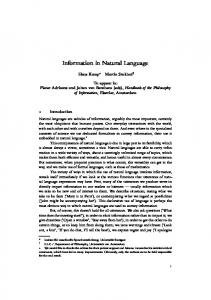
(a)Swaps of 1 and 2 bytes codewords, (b) Swaps of 2 and 3 bytes codewords and (c) Number of new words.
instructions, when an exchange in their codeword lengths is needed to keep the original DETDC compression ratio. Figure 5 shows the pseudocode for the receiver process. Observe that the receiver only has to follow the instructions of the sender, that is, insert new symbols in the words vector (sorted by codewords) when Cnew−symbol arrives, and swap two words in the vector when Cswap arrives.
4.
% 50
EXPERIMENTAL RESULTS
We used some large text collections from trec-2, namely AP Newswire 1988 (AP) and Ziff Data 1989-1990 (ZIFF), as well as trec-4, namely Congressional Record 1993 (CR) and Financial Times 1991 to 1994 (FT91 to FT94). We created two larger corpora ALLFT and ALL by aggregating all texts from FT and of all corpora respectively. As a small collection we use the Calgary corpus. We used the spaceless word model [9] to create the vocabulary, that is, if a word was followed by a space, we just encoded the word, otherwise both the word and the separator were encoded. r Pentium r -III 800 Mhz system, with 768 A dual Intel MB SDRAM-100Mhz was used in our tests. It ran Debian GNU/Linux (kernel version 2.2.19). The compiler used was gcc version 3.3.3 20040429 and -O9 compiler optimizations were used. Time results measure cpu user time in seconds.
4.1 Swaps and evolution of new words Remember that using bytes as target symbols and an ETDC approach, words from position 0 to position 127 are encoded with one byte, words in positions form 128 to 128 + 1282 are encoded with two bytes and so on. With 3 bytes, it is possible to encode more than two millions of words (and vocabularies very rarely will be so huge given Heaps law [12]). Therefore there are two very clear limits in the sorted vocabulary, 128 and 128 + 1282 . These two limits set three intervals. Only when a word changes its position in a way that it changes its ranking interval, the corresponding codeword is modified. Therefore, and this is the key idea, very few changes will occur in the mapping codewords-words. That is, very few swaps will be needed. We compressed collection ZIFF to show how the number of swaps evolves as the text is compressed. The file has 40,627,132 words, and a vocabulary of 237,622 (different) words. In the compression process, 31,772 swaps were produced. This means that only the 0.078% of the frequency changes implied a swap. In addition, most of these swaps were produced in the first stages of the compression, as it can be seen in Figure 4. Note that most of the changes (30,971) are between codewords of size 2 and 3. This is expected since the shape of the Zipf distribution signals a bigger difference in frequency between words 127th and 128th than between words in po-
sitions 128 + 1282 − 1 and 128 + 1282 . Notice that if the word in a position 128 + 1282 − 1 has frequency 1, just one occurrence of any word at position lower than 128 + 1282 will produce a swap. Observe in Figure 4(a) that most of the swaps involving codewords of 1 and 2 bytes take place during the processing of the first 5% of the file. After processing 20% of the file, there are almost no further swaps of this type. Many (about 30%) of the swaps between codewords of 2 and 3 bytes also take place during the compression of the first 5% of the file (see Figure 4(b)). The number of swaps decreases as the compression progresses, showing that the model gets closer to the real distribution as the sample grows. However, the convergence is slower. Figure4(c)) shows that the distribution of new words, as expected, follows a Heaps’ law.
4.2 Compression ratio and efficiency Our implementation of DLETDC uses fixed three-byte values for Cnew−Symbol and Cswap , producing a small lose in compression. If we uses the first two free codewords, we would have saved 2 bytes for Cnew−Symbol in the 127 first new words and one byte in the 1282 = 16, 384 next words. That is, we would have saved 16, 640 bytes for codeword Cnew−Symbol . The same reasoning can be done for Cswap . We have lost exactly 534 bytes by using a fixed three-byte Cswap in the compression of the ZIFF collection shown in Figure 4. These 17, 174 bytes are insignificant in the compressed text size. Table 1 shows the compression ratio we obtained in the different corpora using the two alternatives. Column “Variable” shows the compression ratio reached using the first two free codewords, while “Fixed” refers to using the last two codewords of three bytes. Notice that the loss in compression ratio is insignificant, especially on large files. Corpus CALGARY FT91 CR FT92 ZIFF FT93 FT94 AP FTALL ALL
Size 2,131,045 14,749,355 51,085,545 175,449,235 185,220,215 197,586,294 203,783,923 250,714,271 591,568,807 1,080,719,883
Variable 49.36% 36.16% 32.21% 32.93% 33.87% 32.97% 32.92% 33.17% 32.57% 33.69%
Fixed 50.16% 36.28% 32.24% 32.94% 33.88% 32.98% 32.93% 33.18% 32.57% 33.69%
Table 1: Comparing compression ratios.
The computationally most significant work at the receiver is to process the swap, and as we have shown, the number of swaps occurred is insignificant with respect to the number of words processed. In addition, the number of swaps drops as
Corpus CALG. FT91 CR FT92 ZIFF FT93 FT94 AP FTALL ALL
Gzip DETDC DETDC Arith Bzip2 36,95% 50,16% 47,73% 34,68% 28,92% 36,42% 36,28% 35,64% 28,33% 27,06% 33,29% 32,24% 31,98% 26,30% 24,14% 36,47% 32,94% 32,84% 29,82% 27,09% 33,06% 33,88% 33,79% 26,36% 25,11% 34,21% 32,98% 32,89% 27,89% 25,32% 34,21% 32,93% 32,84% 27,86% 25,26% 37,31% 33,18% 33,11% 28,00% 27,21% 34,94% 32,57% 32,54% 27,85% 25,86% 35,09% 33,69% 33,66% 27,98% 25,98%
Table 2: Compression Ratio. Corpus Gzip DLETDC DETDC Arith Bzip2 CALG. 0.933 0.470 0.384 1.030 2.660 FT91 6.303 2.990 2.488 6.347 18.200 CR 19.767 10.010 8.418 21.930 65.170 FT92 76.313 36.983 31.440 80.390 221.460 ZIFF 71.293 39.370 33.394 82.720 233.250 FT93 77.560 41.823 36.306 91.057 237.750 FT94 73.290 43.703 36.718 93.467 255.220 AP 114.570 54.647 47.048 116.983 310.620 FTALL 234.703 127.745 111.068 274.310 718.250 ALL 431.470 254.910 213.905 509.710 1.342.430
Table 3: Compression time. the model converges, and therefore, since the receiver does very little computation, it is very fast. We empirically compare the compression ratio and compression/decompression speed of DLETDC, against Gzip (a Ziv-Lempel compressor) [23, 24], Bzip2 (a block sorting compressor) [7], an arithmetic encoder [8] and DETDC [5]. Table 2 shows the results on compression ratio. As expected Bzip2 compresses the most and Gzip the least. DLETDC achieves better compression ratios than Gzip except in small collections (Calgary). DLETDC compresses slightly less than DETDC, since the compressed data has to carry information about the swaps. Table 3 shows compression time. Now it is clear that DETDC and DLETDC are by far the best anternatives. Notice that due to the swap management, DLETDC is slightly worse than the DETDC. Table 4 shows decompression times. Remember that Gzip is considered a very efficient technique for decoding, and in fact this is its strength when compared to DETDC and the others. However, DLETDC is never much slower than Gzip and it is clearly faster than Gzip as soon as the collection has a medium size. Hence, DLETDC is easier to program, compresses more, and compresses and decompresses faster Gzip. This is enough by itself to make DLETDC an interesting choice for dynamic compression of natural language texts. However, it has other relevant features, as we show next.
5.
KEYWORD FILTERING Gzip DLETDC DETDC Arith Bzip2 CALGARY 0.067 0.097 0.240 0.973 0.830 FT91 0.673 0.600 1.545 5.527 5.890 CR 2.123 2.013 5.265 18.053 19.890 FT92 7.703 7.850 19.415 65.680 71.050 ZIFF 7.577 7.947 20.690 67.120 72.340 FT93 9.120 8.610 21.935 71.233 77.860 FT94 9.160 8.933 22.213 75.925 80.370 AP 13.057 11.650 27.233 88.823 103.010 FTALL 28.823 25.735 66.238 214.180 235.370 ALL 59.790 49.530 126.938 394.067 432.390
Table 4: Decompression time.
The problem to perform direct search over text compressed with previous dynamic methods is that the codeword, used to encode a specific word, changes many times along the process. Following those changes requires an effort close to that of just decompressing the text and then searching it. Since, as we showed, there are very few swaps, the codeword of each word changes with much less frequency than in the case of previous adaptive techniques. This makes it possible to scan the arriving text looking for some specific patterns. Of course the codewords for those patterns may change along the process. At the beginning of the process, a searched word will appear in ASCII form, preceded by the Cnew−Symbol codeword. At that point the Clast codeword becomes the pattern we must look for to find that word. Latter, that codeword may change again but the Cswap codeword marks each change and, therefore, the scanning algorithm can easily follow the evolution of all the search patterns in the compressed text. Since we have few changes in the codeword-word mapping as we show in Section 4.1, we can apply a Boyer-Moore family search algorithm, which in our experiments has been the set Horspool algorithm [13, 18]. However, we have to consider several special issues when searching DLETDC compressed text. Let us suppose that we are searching for patterns p1 , p2 , . . . , pn . We use P (pi ), 1 ≤ 1 ≤ n to denote the plain version of the pattern and C(pi ) to denote the codeword representing pi in a certain moment. We represented the patterns, both ASCII versions of the words and codewords, using a trie. Initially all the P (pi ) are represented in the trie, but as soon as any P (pi ) appears for the first time in the text, the trie is updated by deleting P (pi ) and inserting the corresponding C(pi ) pattern (which initially is always the current Clast value). Codeword Cswap is also represented in the trie, since the codeword of a search pattern can be changed by the sender using Cswap as the escape codeword. Upon finding Cswap , the algorithm has to read the next two codewords and check if one (or both) of them is in the trie. If it is, the algorithm updates the trie in order to replace the current C(pi ) codeword of a search pattern by its new codeword. Remember that, although we lose some compression, we preferred to use for Cnew−Symbol and Cswap the last threebyte codewords, because this improves the search speed. Both Cnew−Symbol and Cswap must be explicitly represented in the trie, so if we used the first two free codewords to represent them, we would have to update the trie each time a new word arrived, which would be too expensive. On the other hand, a Booyer-Moore pattern matching algorithm takes advantage of longer patterns because it permits skipping more bytes. The use of variable values for Cnew−Symbol and Cswap would yield too short codewords to look for at the beginning of the process. The fixed alternative of three-byte codewords permits longer shifts (unless we search for a frequent word coded with one or two bytes).
5.1 Empirical results on searching We searched, in both the compressed and the uncompressed versions of the text, the same set of patterns chosen at random from the text. We averaged the results over 100 searches, each with different patterns. Patterns that occurred only once in the test were not chosen, to avoid strange elements such as long arrays of separator characters. Table 5 compares search times over corpora of different
Patterns CR AP ALL # len. PlainDLETDC (%) PlainDLETDC (%) PlainDLETDC (%) 5 6 0.47 0.20 42.55 2.40 0.92 38.33 10.14 3.52 34.74 5 1 0.51 0.20 38.83 2.62 0.92 35.30 11.76 3.36 28.61 10 6 0.62 0.21 33.87 3.14 0.98 31.32 13.80 3.46 25.06 10 1 0.73 0.21 28.76 3.60 0.97 26.90 17.12 4.17 24.35 15 6 0.73 0.21 28.76 3.68 1.02 27.71 15.84 4.38 27.64 15 1 0.89 0.22 24.71 4.31 1.01 23.40 19.18 4.33 22.57 20 6 0.80 0.22 27.50 4.09 1.06 25.91 17.61 4.49 25.49 20 1 0.99 0.23 23.23 5.18 1.06 20.56 20.47 4.49 21.93 25 6 0.88 0.35 39.77 4.35 1.26 29.08 18.70 5.01 26.81 25 1 1.12 0.23 20.53 5.57 1.21 21.72 23.14 4.63 20.03
Table 5: Searching in CR, AP and ALL corpora. sizes. The first column gives the number and minimum ASCII length of the search patterns. For each corpus we give the time to search the plain and the uncompressed text, as well as the compressed/uncompressed time fraction. The use of longer patterns obviously improves the search speed in the uncompressed text. However, this has little effect in the search time over the compressed text, as in this case we always search for codes of two or three bytes (rarely shorter, as only 128 words are encoded with just one byte). A more surprising result is that a larger number of patterns favors the search of the compressed over the uncompressed text. Note that handling more patterns does not affect much the search speed in DLETDC compressed text. The main reason is that Horspool algorithm benefits from a lower probability of two characters (from the text and the pattern) being equal. The lower this probability, the more patterns can be handled efficiently. In DLETDC compressed text this probability is close to 1/256 ≈ 0.004, while in plain English text it is known to be around 0.067.
6.
CONCLUSIONS
We have presented Dynamic Lightweight End Tagged Dense Code (DLETDC), a new word-based byte oriented statistical compressor that, as ETDC [6], (sc)-DC [4] and DETDC [5], belongs to the family of dense compressors. DLETDC, as other statistical word-oriented compressors, obtains compression ratios around 32-34% but, being a member of the “dense” family, it is easier to implement and, at the same time, compresses more efficiently. We show that, as soon as the compressed text collection reaches a significative size, DLETDC becomes an interesting alternative because it is more efficient and obtains better compression ratios than DETDC and Gzip. At the same time DLETDC offers an interesting space/time tradeoff that no other dynamic compressor, such as bzip2 or arithmetic encoders, can reach. A very interesting feature of this compressor is that it breaks the usual symmetry between sender and receiver processes, which is common to most adaptive compressors. Two interesting consequences of this asymmetry are: the low computing power required by the receiver, where decompression is remarkably fast, and the possibility of searching the compressed text without decompressing it, uncommon on adaptive scenarios. This second property opens the possibility of scanning the compressed text as it arrives and filtering it by the words it contains to perform classification or retrieval tasks. The possibility of scanning a dynamic compressed text as it is arriving opens a new horizon of possibilities for new applications and environments, such as mobile computing when a source continuously broadcasts information.
7. REFERENCES
[1] R. Baeza-Yates and B. Ribeiro-Neto. Modern Information Retrieval. Addison-Wesley, 1999. [2] T. C. Bell, J. G. Cleary, and I. H. Witten. Text Compression. Prentice Hall, 1990. [3] R. Boyer and J. Moore. A fast string searching algorithm. Comm. ACM, 20(10):762–772, 1977. [4] N. Brisaboa, A. Fari˜ na, G. Navarro, and M. Esteller. (s,c)-dense coding: An optimized compression code for natural language text databases. In Proc. 10th SPIRE, LNCS 2857, pages 122–136, 2003. [5] N. Brisaboa, A. Fari˜ na, G. Navarro, and J. Param´ a. Simple, fast, and efficient natural language adaptive compression. In Proc. 11th SPIRE, LNCS 3246, pages 230–241, 2004. [6] N. Brisaboa, E. Iglesias, G. Navarro, and J. Param´ a. An efficient compression code for text databases. In Proc 25th ECIR, LNCS 2633, pages 468–481, 2003. [7] M. Burrows and D. J. Wheeler. A block-sorting lossless data compression algorithm. Tech.Rep. 124, Digital, 1994. [8] J. Carpinelli, A. Moffat, R. Neal, W. Salamonsen, L. Stuiver, A. Turpin, and I. Witten. Word, character, integer, and bit based compression using arithmetic coding. http://www.cs.mu.oz.au/~alistair/arith coder/, 1999. [9] E. de Moura, G. Navarro, N. Ziviani, and R. Baeza-Yates. Fast searching on compressed text allowing errors. In Proc. 21st SIGIR, pages 298–306, 1998. [10] E. de Moura, G. Navarro, N. Ziviani, and R. Baeza-Yates. Fast and flexible word searching on compressed text. ACM TOIS, 18(2):113–139, 2000. [11] A. Fari˜ na. New Compression Codes for Text Databases. PhD thesis, University of A Coru˜ na, Computer Science Department, A Coru˜ na, Spain, 2005. To appear. [12] H. S. Heaps. Information Retrieval: Computational and Theoretical Aspects. Academic Press, 1978. [13] R. N. Horspool. Practical fast searching in strings. Software Practice and Experience, 10(6):501–506, 1980. [14] D. A. Huffman. A method for the construction of minimum-redundancy codes. Proc. Inst. Radio Eng., 40(9):1098–1101, 1952. [15] A. Moffat. Word-based text compression. Software Practice and Experience, 19(2):185–198, 1989. [16] A. Moffat and A. Turpin. Compression and Coding Algorithms. Kluwer, 2002. [17] G. Navarro, E. de Moura, M. Neubert, N. Ziviani, and R. Baeza-Yates. Adding compression to block addressing inverted indexes. Information Retrieval, 3(1):49–77, 2000. [18] G. Navarro and M. Raffinot. Flexible Pattern Matching in Strings – Practical on-line search algorithms for texts and biological sequences. Cambridge University Press, 2002. [19] G. Navarro and J. Tarhio. Boyer-Moore string matching over Ziv-Lempel compressed text. In Proc. 11th CPM, LNCS 1848, pages 166–180, 2000. [20] A. Turpin and A. Moffat. Fast file search using text compression. In Proc. 20th Australian Computer Science Conf., pages 1–8, 1997. [21] I. H. Witten, A. Moffat, and T. C. Bell. Managing Gigabytes: Compressing and Indexing Documents and Images. Morgan, 1999. [22] G.K. Zipf. Human Behavior and the Principle of Least Effort. Addison-Wesley, 1949. [23] J. Ziv and A. Lempel. A universal algorithm for sequential data compression. IEEE TIT, 23(3):337–343, 1977. [24] J. Ziv and A. Lempel. Compression of individual sequences via variable-rate coding. IEEE TIT, 24(5):530–536, 1978. [25] N. Ziviani, E. de Moura, G. Navarro, and R. Baeza-Yates. Compression: A key for next-generation text retrieval systems. Computer, 33(11):37–44, 2000.