Index Structures for Efficiently Searching Natural Language Text Pirooz Chubak
Davood Rafiei
Department of Computing Science University of Alberta Edmonton, Canada
Department of Computing Science University of Alberta Edmonton, Canada
[email protected]
[email protected]
ABSTRACT Many existing indexes on text work at the document granularity and are not effective in answering the class of queries where the desired answer is only a term or a phrase. In this paper, we study some of the index structures that are capable of answering the class of queries referred to here as wild card queries and perform an analysis of their performance. Our experimental results on a large class of queries from different sources (including query logs and parse trees) and with various datasets reveal some of the performance barriers of these indexes. We then present Word Permuterm Index (WPI) which is an adaptation of the permuterm index for natural language text applications and show that this index supports a wide range of wild card queries, is quick to construct and is highly scalable. Our experimental results comparing WPI to alternative methods on a wide range of wild card queries show a few orders of magnitude performance improvements for WPI while the memory usage is kept the same for all compared systems.
Categories and Subject Descriptors I.7.3 [Document and Text Processing]: Index Generation; H.2.4 [Database Management]: Systems—Query Processing
General Terms Performance
Keywords Indexing natural language text, Querying performance, Wild card queries
1.
INTRODUCTION
Natural language text is pervasive; emails, news-group messages, web pages, research papers, books, news, etc. are almost entirely authored in a human readable natural
Permission to make digital or hard copies of all or part of this work for personal or classroom use is granted without fee provided that copies are not made or distributed for profit or commercial advantage and that copies bear this notice and the full citation on the first page. To copy otherwise, to republish, to post on servers or to redistribute to lists, requires prior specific permission and/or a fee. CIKM’10, October 26–30, 2010, Toronto, Ontario, Canada. Copyright 2010 ACM 978-1-4503-0099-5/10/10 ...$10.00.
language. Such huge volumes of data provide the feed for many applications including search engines, Question Answering (QA) systems, and many analytical tools built on more ad-hoc basis. QA systems in particular are important in that they extract relevant facts and meaningful answers to questions, but mostly deal with relatively small and clean corpora and involve deep and time-consuming natural language processing. Hence, there has been little focus on the performance of such systems on large text collections. This is the topic we study in this paper. In particular, we introduce and evaluate access methods that greatly improve upon the performance of keyword searching for wild card queries over large natural language text collections. The work has a significant impact on many applications where answers to natural language questions are sought or the query includes some wild cards.
1.1 From Natural Language Questions to Wild Card Queries Question answering on a large corpus is a challenging task mainly because it is difficult to analyze the whole (or a good portion of) data and to retrieve candidate answers. On open-domain QA applications, such as question answering over the web1 , it would be very difficult to build a general QA system with high accuracy. In those cases, a reasonable approach is to convert natural language questions into queries and benefit from available querying engines to enhance the performance of the search. The choice of queries can further affect the efficiency of searching, ease of translating questions to queries and the relevance of the results. Table 1 gives a list of query types and some of the contexts where each query type is used. Of those listed, wild card queries, where keywords matching a wild card are sought, are particularly important for several reasons. First, a large number of natural language questions can easily be translated into one or more wild card queries. As an example who and what questions and a large number of which and where questions can be translated into wild card queries (See Table 2). Second, the results of such queries can easily be joined with data that may reside in a database. For example, candidate answers for the which question in Table 2 can be further refined by looking up the values returned by the first query in a database populated with a list of city names (second query). Finally, question answering systems often rely on NLP components that may directly or indirectly use wild card queries. Examples are taxonomy construction, fact extraction, named entity recog1
See OpenEphyra [7] for an example
Table 1: Summary of the literature Query Type Query Elements Keyword queries keywords, Boolean operators Multi-keyword queries keywords, phrases Proximity queries keywords, proximity radius Wild card queries queries, wild cards(%) Structured queries SQL, text predicates
on query types Result Set documents documents documents list of keywords relations
Full-text search
strings
characters, regular expressions
nition and query expansion. Rafiei and Li [28] present wild card querying over web text and discuss several techniques such as query expansion and relevance ranking to increase the precision and recall of extractions. Table 2: Samples of natural language questions and their corresponding wild card queries Question Who invented the light bulb? What is glass made of? Which city hosted 1988 Olympics? Where is Grand Canyon located?
Translation % invented the light bulb glass is made of % % hosted 1988 Olympics % is a city Grand Canyon is located in %
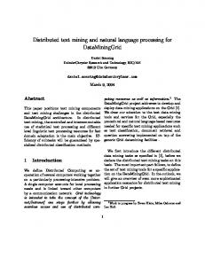
There has been a great deal of activity around increasing the efficiency of keyword-based queries. However, the same structures and algorithms would not necessarily be useful or efficient for evaluating wild card queries. Assume we are given an inverted index structure, such as the one depicted in Figure 1 with four terms and three documents. Each term t in the index has a list of postings, each posting in the form of a triplet < d, ft,d , [o1 , · · · , oft,d ] > where d is a document id, ft,d is the frequency of t in d and o1 · · · oft,d are offsets in d where t appears. Given a keyword query Q1:‘world population’ and a wild card query Q2:‘world population is %’, the algorithm for evaluating Q1 involves only intersecting the posting lists of terms ‘world’ and ‘population’, and finding the list of matching documents. However, for Q2, each matching document has to further be scanned in order to find the keywords that match the wild card. In the above example, Q1 matches , and , and Q2 matches ‘6706993152’ which is located on offset 10 of document 3. Although Q2 matches its answer in fewer documents than Q1, the query response time for Q2 using inverted indexes in one of our experiments was 12 times larger. This indicates that inverted indexes are not appropriate for evaluating wild card queries. 6706993152 → is →, ,
population →, ,
world →, ,
Figure 1: Architecture of an inverted index Solutions on multi-keyword queries such as phrase and nextword indexes [11, 30] can help reduce the time it takes
and their result sets References AltaVista [1], Google [4], Yahoo [8] [17], [11, 30] Lucene [2], INDRI [5], [16] Dewild [28], BE [14], KnowItAll [18] Oracle InterMedia Text[9], DB2 Text Extender[24], [15]
to intersect the posting lists, but won’t help in the keyword matching step, which is in most cases the dominant process. Therefore, development of solutions for efficient retrieval of keyword matches from text seems essential.
1.2 Our Contributions and the Structure of the Paper In this paper we introduce Word Permuterm Index (WPI), as an efficient index structure for evaluating wild card queries over natural language text. WPI extends Permuterm Index (PI) [22] in several aspects. (1) By construction, WPI supports pattern matching over keywords rather than characters, (2) WPI supports a wider range of queries than PI, adding support for queries that are more frequently used over natural language text, and (3) WPI returns the actual keywords that match a wild card query whereas PI is mostly used to find the range of elements that match a pattern. Thus, WPI goes one more step toward matching the keywords after finding the range of matching elements. Our other contribution is a broad set of experiments and analyses comparing the performance of WPI to alternative stateof-the-art methods. Our performance comparison includes cases where WPI is given a limited memory and is forced to do paging. To the best of our knowledge this is the first work that experimentally compares traditional inverted file indexes with more recent compressed full-text indexes (See the survey in [26]). The rest of this paper is structured as follows. In Section 2 we describe the different index structures in the literature and how they can be utilized to solve the wild card querying problem. In Section 3 we detail our solution and give a theoretical comparison with the previous approaches. In Section 4 we provide comprehensive comparison among these structures and their performance. A review of the literature on different query types, index structures and querying algorithms are given in Section 5. Finally we conclude and provide remarks for future work in Section 6.
2. BASELINE METHODS Without loss of generality, we consider phrase queries that have exactly one wild card and any number of non-wild card terms, referred to as literals. For queries with multiple wild cards, one can find the matches for query sub-sequences that have only one wild card, substitute the wild card with its matches and look for further matches. Next, we introduce a few baseline access methods that are used within natural language applications and study their performance. Regardless of the access strategy, a wild card query evaluation can be often divided into two phases: (1) Binding phase, where the indexed elements (e.g. sentences, paragraphs or documents) are filtered based on the
query literals that are present and maybe their order, and (2) Matching phase in which filtered elements are scanned and the keywords that match the wild card are retrieved.
2.1 Full Scan A straightforward approach for answering wild card queries is to scan the full dataset and check every unit for possible query matches. If the dataset fits in main memory, a full scan may not be a bad idea given that the initial cost of loading is negligible when amortized over a reasonable-sized set of queries.
2.2 Inverted Index As illustrated in Figure 1, our implementation of an inverted index stores a linear vector of posting triplets < d, ft,d , [o1 , · · · , oft,d ] >. Wild card query evaluation over inverted index can be easily adapted from the standard implementations of keyword queries. Keyword queries are evaluated by intersecting the posting lists of query literals and finding the matching documents and corresponding offsets. The key idea behind wild card query evaluation is to sequentially scan these documents and to find and extract the wild card matches. Thus, in order to do the wild card matching we need to store and access the text dataset as well. The complexity of wild card matching over an inverted P index is O( m i=1,qi 6=% kqi k) + O(kQk · |davg |), where kP k is the number of bindings of a pattern P 2 . Since we have to go through all the matching elements in order to find the wild card matches, the cost is kQk · |davg |, where davg is the average size of an index element.
2.3 Neighbor Index Neighbor index, as proposed by Cafarella and Etzioni [14], is an inverted index that is more suitable for queries over natural language text data. The index stores for each term both its left and right neighbors. As shown in Figure 2 for our running example (given in Figure 1), the inverted lists have grown significantly larger, but the answer to wild card matches are stored within the index and can be found by looking at the appropriate neighbors of a query literal. For example, to find the matches for Q2 in the neighbor index, the search is conducted in the inverted index until offset o = 10 in document d = 1 is identified as an answer. To obtain the actual answer, it is sufficient to look at the right neighbor of the term at offset 9 in the index without retrieving the document. This can speed up the evaluation of wild card queries by 1-2 orders of magnitude compared to inverted index, as reported by the authors and confirmed in some of our experiments. The original implementation of the neighbor index stores for each neighbor in addition to the term, both its part of speech (e.g. noun-phrase) and its role (e.g. term). Since the tags are not explicitly used in our queries, we implemented a simplified version of the neighbor index, where for each offset, only one left neighbor and one right neighbor were stored with no further information. Therefore, the structure of a posting in our implementation of the neighbor index looked like < d, ft,d , [(o1 , l1 , r1 ), · · · , (oft,d , lft,d , rft,d )] >, where li and ri are the left and right neighbors of the i’th occurrence of t in d, respectively. Given that neighbor index is an inverted index, the algo2
The number of documents matching P
rithm for evaluating wild card queries over neighbor index follows the same bind-and-match process of any inverted index, except that the matching phase is much less costly. Once the matching documents and offsets are found, the wild card matches can be extracted in constant time. Thus, the running time of wild P card query evaluation over a neighbor index will be O( m i=1,qi 6=% kqi k) + O(kQk).
3. PERMUTERM INDEX OVER NATURAL LANGUAGE TEXT This section presents our Word Permuterm Index (WPI) as an efficient access method that supports wild card querying over natural language text. WPI is an adaptation of the permuterm index [22, 21] and as such it has the following three components: (1) A word level Burrows-Wheeler (BW) transformation of text [13], (2) an efficient mechanism to store and access the alphabet, and (3) an efficient mechanism to access the ranks. Next, we discuss these components in more detail.
3.1 Word Level Burrows-Wheeler transformation Burrows-Wheeler transformation (BWT) is a reversible transformation that is used in well-known compression algorithms such as bzip2 and is believed to give a permutation that is more amenable to compression. The transformation, when applied to a character string, can change the ordering of the characters in the string but not their values. Our work applies BWT to words instead of characters; a word-level transformation has some interesting properties especially in answering wild card queries. Assume we are given a dataset containing three sentences S1: ‘Rome is a city’, S2: ‘countries such as Italy’ and S3: ‘Rome is the capital of Italy’, and we would like to index them using WPI. Adapting the ideas proposed by Manning et al. [25] and Ferragina and Venturini [21], we sort this dataset lexicographically3 and use the $ symbol, to mark the sentence boundaries and the e symbol, to mark the end of the dataset. This results in our dataset to look like T: ‘$ Rome is a city $ Rome is the capital of Italy $ countries such as Italy $ e’.
A word-level BWT is obtained by (1) computing all the cyclic rotations of the words, (2) sorting the rotations, and (3) finding the vector that contains the last word in the rotations in the same order after the sorting. Figure 3 depicts the result of applying these three steps to T in the given example. Note that the set of sentences are rotated by one word at each level. We denote the vector of last words, BWtransformation, by L and the sorted vector of first words, by F . BWT has some very interesting properties. First, for any word in T , the j’th occurrence of the word in L and the j’th occurrence of the word in F correspond to the same word of the sequence. For instance, the second occurrence of the word ‘Italy’ in L is preceded by ‘as’, and so is the second ‘Italy’ in F ; hence, L(4) = F (6). Second, for every row, L(i) precedes F (i) in T . Given these two properties, Ferragina and Manzini [20] propose the following function for traversing L in backward order: LF (i) = C[L[i]] + RankL[i] (L, i) 3
Sorting guarantees nice properties on BWT, See Section 3.4
6706993152 → is →, , population →, , world →, , 1
Document Boundary Marker
Figure 2: Architecture of a neighbor index
i
F
L
1 2 3 4 5 6 7 8 9 10 11 12 13 14 15 16
Rome is a city $ Rome is the capital of Italy $ countries such as Italy $ ~ $ Rome is the capital of Italy $ countries such as Italy $ ~ $ Rome is a city $ a city $ Rome is the capital of Italy $ countries such as Italy $ ~ $ Rome is as Italy $ ~ $ Rome is a city $ Rome is the capital of Italy $ countries such capital of Italy $ countries such as Italy $ ~ $ Rome is a city $ Rome is the city $ Rome is the capital of Italy $ countries such as Italy $ ~ $ Rome is a countries such as Italy $ ~ $ Rome is a city $ Rome is the capital of Italy $ is a city $ Rome is the capital of Italy $ countries such as Italy $ ~ $ Rome is the capital of Italy $ countries such as Italy $ ~ $ Rome is a city $ Rome of Italy $ countries such as Italy $ ~ $ Rome is a city $ Rome is the capital
17 18 19
such as Italy $ ~ $ Rome is a city $ Rome is the capital of Italy $ countries the capital of Italy $ countries such as Italy $ ~ $ Rome is a city $ Rome is ~ $ Rome is a city $ Rome is the capital of Italy $ countries such as Italy $
$ Rome is a city $ Rome is the capital of Italy $ countries such as Italy $ ~ $ Rome is the capital of Italy $ countries such as Italy $ ~ $ Rome is a city $ countries such as Italy $ ~ $ Rome is a city $ Rome is the capital of Italy $ ~ $ Rome is a city $ Rome is the capital of Italy $ countries such as Italy Italy $ countries such as Italy $ ~ $ Rome is a city $ Rome is the capital of Italy $ ~ $ Rome is a city $ Rome is the capital of Italy $ countries such as
Figure 3: Sorted permutations of a sample set of sentences and the first and last word lists, F and L. where C[L[i]] is the number of words smaller than L[i] and RankL[i] (L, i) is the number of times L[i] appears in the sub-sequence L[1..i]. LF (i) tells where the element preceding L[i] in T is located in L. E.g. LF (6) = C[′ as′ ] + Rank′ as′ (L, 6) = 9 + 1 = 10 and L(10) is ‘such’ and is the word preceding L(6) =‘as’ in T . Since T is sorted, one can start from L(1) = F (n) and repeatedly call LF to find L(n) = F (1), traversing the whole text in backward order. Therefore, L is reversible, meaning that given L, any sub-sequence of words in T can be re-constructed. We can use this property to turn L into an index that can support searches over word sequences. The challenges would be to support a wide range of wild card queries and to efficiently support access to C and Rank, required for traversing L in backward order. Next, we discuss these challenges and the proposed solutions.
3.2 Maintaining the Alphabet A major difference between the permuterm index and WPI is in the size of their alphabets. The alphabet in permuterm index typically consists of ascii characters and symbols which are small in size and are not required to be explicitly stored. However, the alphabet size in WPI grows with the size of text dataset almost linearly. When |Σ| is in the order of millions, efficient access to alphabet elements, their ordering and their frequency is crucial. In order to provide efficient access to Σ, we built one array and one hash table. The array stores the elements of
Σ in ascending order, therefore the first element is always $ and the last is e. The array helps to find which alphabet element is represented by which numerical code, which is its index in the array. Coding the alphabet is essential for efficient implementation of algorithms such as backwardSearch and Rank. Without coding, we will not be able to achieve the time complexities we later report for these algorithms. Moreover, coding reduces the index size, replacing a keyword and a delimiter by a code which uses smaller number of bits. The hash table stores the same information in the reverse order; given an alphabet element, the hash returns the code of the element, together with its frequency and cumulative frequency, C. Thus, C[t] counts the number of alphabet elements in the whole dataset that are smaller than t. In the above example, |Σ| = 13 and the hash table provides constant-time access to C values for all the alphabet elements.
3.3 Rank Data Structures Rankc (L, i) returns the number of occurrences of c ∈ Σ in the prefix 1 · · · i of array L. In order to evaluate queries over WPI, we make frequent accesses to Rank and therefore, quick access would be required. Naive baseline solutions to the rank problem are as follows. (1) Start from the first element on L and compute rank by counting, which has space complexity and average search complexity of O(n). (2) Keep a matrix of all the alphabet elements and all the locations
on L and pre-compute all the values. This approach has the optimal constant search time but a space requirement of O(n|Σ|), which is too much given the fact that |Σ| grows relative to the size of the dataset. Given the large size of our alphabet, we chose a combination of a wavelet tree [23] and a three level architecture to support constant time rank operation over a bit sequence [26]. A wavelet tree is a perfect binary tree, with a bit sequence at each node representing the occurrences of a sequence of alphabet elements. The root represents Σ over L and each leaf represents one of the alphabet elements. A non-leaf node v represents alphabet elements Σv = {ei · · · ej } and contains a bit sequence Bv = bi · · · bj . For each i ≤ k ≤ j we have bk = 0, if L[k] ∈ {ei · · · e(i+j)/2 } and bk = 1, if L[k] ∈ {e(i+j)/2+1 · · · ej }. The bit sequence at the left child of v will represent elements of Σ in {ei · · · e(i+j)/2 } and the right child represents alphabet elements {e(i+j)/2+1 · · · ej }, recursively. Thus, the algorithm for computing rank of an alphabet element e ∈ Σ in prefix 1 . . . i of L, using the wavelet tree, would be as shown in Figure 4. Rank(Node,f,l,e,i) 1 if i = j return nodeRank(Node,i) else 2 if e ≤ ⌊ f +l ⌋ 2 ⌋, e, i - nodeRank(Node,i)) 3 return Rank(Node→left, f, ⌊ f +l 2 else 4 return Rank(Node→right,⌊ f +l ⌋+1,l, e,nodeRank(Node,i)) 2
Figure 4: Rank function computes the occurrences of e
nodeRank(Node,e,i) 1 Rsbr = sbr[⌊ Si2 ⌋], Rbr = br[⌊ Si ⌋] b
b
2 if i − Sb × ⌊ Si ⌋ < t b 3 Rsr =sr[b2d(Node→bs,Sb × ⌊ Si ⌋,t)][i-Sb × ⌊ Si ⌋-1] b b 4 else if i − Sb × ⌊ Si ⌋ = t b 5 Rsr =sr[b2d(Node→bs,Sb × ⌊ Si ⌋,t)][t-1] b 6 if i − Sb × ⌊ Si ⌋ > t b 7 Rsr =Rsr +sr[b2d(Node→bs,Sb × ⌊ Si ⌋+t,t)][i-Sb × ⌊ Si ⌋-t-1] b
b
Figure 6: A constant-time nodeRank, returning binary rank at each node
tion 3.1 and propose backwardSearch algorithm, which searches for a pattern over PI in backward order and returns the range of matching strings. The term-level adaptation of backwardSearch over WPI is depicted in Figure 7. Given a sequence of natural language words P = p1 · · · pq , backwardSearch finds the range [f irst, last] of the sorted cyclic rotations prefixed by P . For the example provided in Figure 3, backwardSearch returns the range [7, 8] for the pattern P = ‘Rome is’, which is the range of cyclic rotations prefixed by P . backwardSearch makes O(|P |) accesses to C and Rank. We adjust the hash table size so that it provides constant time access to hash elements. The wavelet tree access for Rank requires traversing from the root to one of the leaves which requires O(log |Σ|) accesses to the tree nodes. Thus, backwardSearch has a complexity of O(|P | log |Σ|).
in prefix 1 . . . i of L backwardSearch(P )
In Figure 4, nodeRank(N ode, e, i) counts the number of 1’s in the prefix 1 . . . i at node N ode. The count of 0’s can be obtained by i−nodeRank(N ode, e, i). Counting the number of 1’s in each node by sequential scanning is very in-efficient. There are a few solutions, that provide constant-time access to binary rank values over a bit sequence [26]. In our work, we used a solution which uses n+o(n) bits of additional storage at each node, where n is the length of the bit sequence in the node. Figure 5 depicts our wavelet tree solution over L for the example of Section 3.1. For the nodeRank to operate in constant time, two arrays are maintained at each node, namely sbr and br4 . For each node, sbr[i] stores the count of 1’s in the range [b0 . . . bi×S 2 −1 ], where Sb = ⌈log n⌉ and b i ∈ {0 . . . ⌊ Sn2 ⌋}. br[i] stores the count of 1’s for the range b
[b⌊ i×Sb ⌋×S 2 . . . bi×Sb −1 ]. Finally, a table called Small Rank S2 b
b
(sr) is pre-populated, which stores the binary rank values for bit sequences of size t = ⌊Sb /2⌋ + 1. Recall that nodeRank function returns the rank of a prefix of the bit string stored at a given node. As depicted in Figure 6, nodeRank uses sbr, br and sr arrays to compute the rank in constant time. nodeRank is computed as shown in Figure 6. In this figure, b2d(bs, p, len) returns the decimal equivalent of the bit sub-sequence bsp . . . bsp+len .
3.4 Algorithms and Analysis Ferragina and Manzini in [20] benefit from the properties of the Burrows-Wheeler transformation discussed in Sec4 These stand for super block rank and block rank, respectively
1 2 3 4 5 6 7 8
i = |P |, c = P [i], f irst = C[c] + 1, last = C[c + 1] while ((f irst ≤ last) and (i ≥ 2)) do c = P [i] if 1 ≤ f irst ≤ M , increment first. Same for last f irst = C[c] + Rankc (L, f irst − 1) + 1 last = C[c] + Rankc (L, last) i=i−1 return the range [first, last]
Figure 7: backwardSearch algorithm for traversing L in backward order Adding delimiters and sorting stings as discussed in Section 3.1, permuterm index supports wild-card pattern matching over dictionary strings. More specifically, it supports (1) Prefix ($α%), (2) Suffix (%β$), (3) Substring (γ) and (4) PrefixSuffix ($α%β$) queries where α, β and γ are arbitrary sequences of characters [21]. We adapted the above four queries to wild-card keyword matching over natural language text. Thus in our queries α, β and γ are sequences of natural language text words. Moreover, we have added support for queries such as (5) α%, (6) %β, (7) α%β, (8) α%β$ and (9) $α%β where α or β could be in arbitrary places in the document. The set of queries supported by PI are very limited and we often need to search for natural language patterns that are neither a prefix nor a suffix in a document. The key idea behind supporting wild card queries using backwardSearch is to convert them into prefix searches over rotations. Table 3 gives a summary of how to evaluate wild card queries using backwardSearch. In this table, the columns from left to right display the different types of
sr 000 001 010 011 100 101 110 111
0 0 0 0 0 1 1 1 1
1 0 0 1 1 1 1 2 2
2 0 1 1 2 1 2 2 3
1000100011100000110
0 0
2
4
5
100100000010 0 0 2 2
000010110 0 0 1
1001100 0 0 3
100 0 0
1000 0 0
city
110000 0 0 $
100
Italy Rome
1111 0 0
11 0 0
01
0 0
2
0 0
11
a
0 0
1
as
0 0
1
of
1
0 0
101 0 0
0 0 capital
0 0
1
100 0 0
countries
0 0
1
~
1 0 0 is
0 0
11
01 0 0 such
0 0
1
1 0 0 the
0 0
1
Figure 5: A sample wavelet tree. In each node a bit string and two arrays ,super block rank and block rank, are stored. queries supported by WPI, the pattern(s) to invoke backwardSearch with, the range of wild card keyword matches, and the time complexity of the query evaluations, respectively. As displayed in this table, the first six queries could be matched with only one call to backwardSearch, while the last three require two invocations of backwardSearch as the sequence of words are separated by a wild card. For these queries, f irstα and lastα are the beginning and end of the range returned by backwardSearch when invoked by α. Recall that backwardSearch returns only a range of matching rotations, prefixed by a given pattern. Therefore, it does not provide any efficient support for extracting keyword matches for a wild card. We solved this problem by storing two additional lists, T and IF , where IF is the list of locations of elements of F over T ; hence T [IF [i]] = F [i]. These lists require O(n) extra space. However, since the overall space consumption of the index is O(n log |Σ|), storing these additional lists will not change the space complexity of WPI.
4.
EXPERIMENTAL RESULTS
4.1 Experimental Setup For the experiments we used all or parts of the following two text collections. (1) News Dataset is the AQUAINT corpus of English News Text [3], which we processed and extracted the sentences to be indexed. It contains around 18 million sentences and its size is more than 2 GBs. (2) Web Dataset is our crawl of the web done on May 2008, which contains around 2 million documents and is around 8 GBs in size. We created three sets of wild card queries. (1) WHQ query-set was created by replacing the wh keywords in who and what questions from AOL query log [27] with a wild card. (2) SVO query-set was generated by randomly replacing the subject or the object of a Subject-Verb-Object rela-
tion with a wild card. We obtained the SVO relationships using the minipar dependency parser [6]. Finally, (3) n-gram query-set was generated by randomly replacing a keyword with a wild card in an n-gram, with n = 1..5. These n-grams were selected according to their number of bindings in our datasets, in an attempt to cover a wide range of bindings. WPI is a memory-based index, hence to be fair to other indexes we assigned in our experiments as much cache to the inverted and neighbor indexes as the memory used by WPI. We ran each query multiple times and only considered the last running time, in order to make sure cache is being utilized by the querying engine. Neighbor and inverted indexes were implemented over Berkeley DB, with the terms as the keys and posting lists as values.
4.2 Performance of Querying Our first set of experiments compared the performance of the indexes under different settings, in terms of the average running time of queries in seconds. Table 4 gives a summary of the performance of each index over 10 million sentences of news data and 1 million documents of the web data and all the query sets. As Table 4 suggests, WPI performs the best among all indexes on any combination of data and query sets. The third row of the table shows the average number of bindings per query for each query and data set used. Neighbor index performs relatively good when the number of bindings are high. Inverted index performs very poorly on queries that match a large number of documents. MemScan performs relatively slow regardless of what type of query is given. The statistical correlation of the running time of queries over indexes is largest for inverted index and smallest for WPI. These correlations reflect how the indexes perform when the number of bindings grow. Figures 8 and 9 depict the behavior of these four methods with respect to the number of bindings
Table 3: Running queries of different types and the analysis of their complexity Q P wild card match Complexity (1)$α% $α T [IF [first]+|$α|]..T [IF [last]+|$α|] O(|$α| log |Σ|) (2)%β$ β$ L[first..last] O(|β$| log |Σ|) (3)γ γ matches documents1 O(|γ| log |Σ|) (4)$α%β$ β$α L[first..last] O(|β$α| log |Σ|) (5)α% α T [IF [first]+|α|]..T [IF [last]+|α|] O(|α| log |Σ|) (6)%β β L[first..last] O(|β| log |Σ|) (7)α%β α, T [IF [firstα ]+|α|]..T [IF [lastα ]+|α|], kαk ≤ kβk O[(|α|+|β|) log |Σ|] + β T [IF [firstβ ]-1]..T [IF [lastβ ]-1], kαk > kβk O[min(kαk|β|, kβk|α|)] (8)α%β$ α, T [IF [firstα ]+|α|]..T [IF [lastα ]+|α|], kαk ≤ kβ$k O[(|α|+|β$|) log |Σ|] + β$ T [IF [firstβ ]-1]..T [IF [lastβ ]-1], kαk > kβ$k O[min(kαk|β$|, kβ$k|α|)] (9)$α%β $α, T [IF [firstα ]+|$α|]..T [IF [lastα ]+|$α|], k$αk ≤ kβk O[(|$α|+|β|) log |Σ|] + β T [IF [firstβ ]-1]..T [IF [lastβ ]-1], k$αk > kβk O[min(k$αk|β|, kβk|$α|)] 1
See displayString in [21] for details
6
Table 4: Summary of the performance of the indexes in terms of the running time in seconds
Avg
Web data 1M documents n-gram WHQ SVO 5.4e+5 5.1 220 3e-6 2e-6 4e-6 1.34e-4 0.274 0.013 0.01 0.064 0.022 30.8 29.4 29.7 0.06 0.01 0.02 194 8.98 10.2 4.6e+4 4.03 35.8 219.8 116 33.2 6.8e-4 2.5e-4 3e-4 5.42 1.44 0.77 1.2e+3 0.75 1.66 44.9 31.3 30.7
MemScan(0.68) WPI(−0.02) Neighbor(0.66) Inverted(0.99)
4
10 Query running time in seconds (logscale)
Max
Min
News data 10M sentences n-gram WHQ SVO Avg Bindings 2.5e+5 0.4 3.3e+3 WPI 2e-6 1e-6 4e-6 Neighbor 1e-4 0.008 0.005 Inverted 0.03 0.007 0.028 Memscan 82.0 86.6 83.5 WPI 0.03 2.5e-4 2.6e-4 Neighbor 24.0 10.0 4.30 Inverted 1.6e+4 8.99 493 Memscan 431 432.9 424.8 WPI 3.5e-4 6.6e-5 1.2e-4 Neighbor 1.37 0.93 1.20 Inverted 373 0.73 9.71 Memscan 87 90.5 87.47
10
2
10
0
10
−2
10
−4
10
−6
10
0
10
of a query, plotted over 100 n-gram queries over 10 million sentences of news data and 1 million documents of web data, respectively. As these figures show, the running time of WPI is almost entirely independent of the number of bindings of the query. For the data presented in these figures, on average WPI is 5 orders of magnitude faster than the neighbor index. The worst case performance of WPI is still an order of magnitude faster than the neighbor index whereas in its best case, WPI is 6-7 orders of magnitude faster. The worst case, observed as a spike in Figures 8 and 9 for the running time of WPI, belongs to the query ‘the % of’. The running time of WPI on this particular query is relatively higher because the query is of type α%β whose running time complexity is decided by kαk and kβk according to Table 3. Since α=’the’ and β=’of’ are the two highest selective words in the alphabet, we observe the spike in these two figures. In order to compare the scalability of the indexes we conducted another experiment to compare how the indexes perform as the dataset size grows. Figure 10 shows the total querying time of the four indexes over 1000 SVO queries computed over web datasets of size 0.4, 0.8, 1.2, 1.6 and 2 million documents. As this figure shows, the running time of WPI stays almost constant. Starting as low as 0.095 seconds for 0.4 million documents and going up to at most 0.118 seconds for 2 million documents, WPI shows only 24% growth in the overall querying time. The running times of neighbor and inverted indexes grow almost linearly with the dataset size. The minimum (maximum) running times
2
4
6
10 10 10 Number of bindings of a query (logscale)
8
10
Figure 8: The performance of the indexes based on the number of bindings of queries over 10 million sentences of news data are 370 (1693) and 600 (2211) for neighbor and inverted indexes, respectively. Finally, MemScan shows an exponential growth with respect to the dataset size. The maximum running time (for 2 million documents) shows almost two orders of magnitude growth with respect to the minimum running time of MemScan.
4.3 WPI Performance with Limited Physical Memory Given that WPI is a memory-based index, it is important to evaluate its performance in settings where the space consumption of WPI exceeds the available system physical memory. This is a worst-case scenario for WPI whereas inverted and neighbor indexes are not expected to be affected much by limitations on the size of memory. A straightforward solution would be to use disk as a supplementary storage and allocate more memory than available and let the operating system do the paging5 (i.e. decide which memory blocks to swap with disk). In an attempt to push WPI to 5 the terms swapping and paging are used interchangeably in this paper
6
10
6
10
5
2
10
0
10
−2
10
−4
10
−6
10
0
10
2
4
6
10 10 10 Number of bindings of a query (logscale)
8
10
Figure 9: The performance of the indexes based on the number of bindings of queries over 1 million documents of web data do paging, we ran a set of experiments on the news data of sizes 4, 6, 8, 10, 12, 14, 16 and 18 million sentences and web data of sizes 0.4, 0.8, 1.2, 1.6 and 2 million documents. We used a machine with 4 GBs of physical memory, around 0.8 GB of which was reserved by a distribution of the Linux operating system for kernel and other system processes. We report here the amount of memory that was required for storing all data structures required by WPI, as a percentage of the available system physical memory. These memory requirements are depicted on the horizontal axis of Figures 11 and 12 for different sizes of data. The reported values are not the peak memory usage of operating system for WPI process as the process needed additional memory for code, stack and other static and dynamic data items. Hence, the amount of memory the process required exceeded the above figures, and paging could happen for the smaller datasets as well. Figures 11 and 12 show the total running time of 1000 SVO queries over WPI and neighbor index as the datasets vary in size. As Figure 11 shows, WPI’s running time grows dramatically as its size grows to 80% of the memory size. This shows the effect of paging on the WPI process. Moreover, as the figures show, even when paging happens, the running time of WPI is still much lower than the neighbor index. By increasing the swap size, we were able to run WPI over datasets that required memory equal to approximately 10 times that of the available system memory. For large datasets, a major part of the index resides over disk and increasing the dataset size, as our results suggest, does not dramatically change the running time of the queries. Even with such a naive disk-based solution to WPI, it performs pretty well and can scale up well with limited available memory. The total running times of queries for the inverted index and MemScan exceed those of the neighbor index in Figures 11 and 12 and have been omitted for brevity.
4.4 Index Construction Time Table 5 shows the time required to construct WPI compared to neighbor index for our experiment in Section 4.3.
Total running time of 1000 svo queries in seconds (logscale)
4
Query running time in seconds (logscale)
10
MemScan(0.90) WPI(−0.02) Neighbor(0.62) Inverted(0.99)
10
WPI Neighbor Inverted Memscan
4
10
3
10
2
10
1
10
0
10
−1
10
−2
10 400K
800K 1.2M 1.6M Dataset size in terms of the number of documents
2M
Figure 10: Scalability of the indexes over web data of growing sizes. As this table suggests, the construction time of WPI is smaller than neighbor index for the given sets of data. In most cases, inverted index has a slightly lower construction time than WPI and memory scan can be considered as having no construction time except loading the dataset once into the main memory. Table 5: Index construction time of WPI compared to the neighbor index in seconds News dataset sentences 4M 6M 8M 10M 12M 14M WPI 457 689 796 1172 2191 2246 Neighbor 871 1439 2028 2265 3170 3853
5. RELATED WORK Querying over natural language text is often addressed in the literature by indexes that are based on inverted lists. For large text corpora, these indexes run into the problem of high costs of intersecting long posting lists. As a result, solutions for multiple keywords have been proposed that materialize posting lists for more than one keyword. Examples are the works on phrase index and nextword index [11, 30]. Phrase index extracts natural language phrases from a query log and stores inverted lists for such phrases. A nextword index, for each term, keeps a list of high frequency terms that follow it in the text and the pair’s corresponding inverted list. Chaudhuri et al. [17] propose breaking long posting lists into smaller ones by storing lists for multiple keywords. As a result they can guarantee an upper bound for the worst case running time of the queries. The above works have no support for wild card queries. However, it would be interesting to compare the performance of these systems on keyword queries with WPI. Recently, there has been an evolving trend in developing indexes supporting fast sub-string searches over large
2000
1200 WPI Neighbor
WPI Neighbor
Total running time of 1000 SVO queries (seconds)
Total running time of 1000 SVO queries (seconds)
1800
1600
1400
1200
1000
800
600
400
1000
800
600
400
200
200
0
55%
80%
105%
129%
154%
179%
204%
230%
WPI memory consumption in terms of available system physical memory
0
253%
419%
592%
776%
945%
WPI memory consumption in terms of available system physical memory
Figure 11: The performance of WPI vs. neighbor index using paging on News Data of sizes 4, 6, 8, 10,12, 14, 16 and 18 million sentences
Figure 12: The performance of WPI vs. neighbor index using paging on Web Data of sizes 0.4, 0.8, 1.2, 1.6 and 2 million documents
text corpora. As a result, self-indexes6 have been developed and many interesting problems associated with them have been proposed or solved [26]. One of the key ideas that led to the development of such indexes have been the idea of the Permuterm Index by Garfield [22]. Burrows-Wheeler transformation [13] discussed in Section 3.1 uses Garfield’s permuterm index to build a self-index that is highly compressible. Ferragina and Manzini [20] propose algorithms for searching patterns over BWT in time proportional to the length of the pattern. In order to do that, they benefit from constant time access to structures such as Count and Rank. As discussed by Navarro and Makinen in a survey on compressed full-text indexes [26], different structures could be used to provide constant-time access to Rank over a fixed size alphabet. For large variable size alphabets, as is the case for WPI, wavelet trees [23] are proposed. WPI benefits from the above ideas for solving full-text search over strings to improve querying over natural language text. More space efficient implementations of nodeRank function have been reported in [29]. Similar to WPI, keyword-based generalizations of text index structures such as suffix arrays [19] and suffix trees [10] have been developed. Finally, Manning et al. [25] propose solutions for wild card queries with more than one wild card over Permuterm Index. They use the similar concept of materializing the range of matching rotations for one substring of query literals and intersecting with the results obtained from the prefix range returned by the rest of the query literals. Storing T and IF , we would be able to answer queries with arbitrary number of wild card over WPI. There’s a great deal of recent activity around compressing indexes that support full-text search. This emergence has been started since the introduction of the Burrows-Wheeler transformation in 1994 which has a high compressibility and is reversible, making it a good candidate for building a selfindex. The state of the art research in this area suggests indexes that are nearly optimal in size and search time. Ferragina and Venturini [21] proposed Compressed Permuterm
Index (CPI). CPI benefits from the high compressibility of the Burrows-Wheeler transformation. They propose the full indexing algorithms and asymptotic analysis and study the performance of CPI under different compression techniques and how it compares with other indexes such as a trie. There is also work on compressing natural language text databases in [12], suggesting high compression ratios are achievable. We did not dig into the subject of compression over our WPI and focused more on efficiency of indexing. However, since we are using the same concept of BW-transformation, our index could also benefit from the results achieved in this domain.
6
an index which could replace the text
6. CONCLUSIONS AND FUTURE DIRECTIONS We discussed the development of Word Permuterm Index (WPI) which supports single wild card natural language queries. WPI fills in the gaps for a time-efficient index supporting a wide range of wild card queries over natural language text. In this paper we presented our data structures and algorithms. Our asymptotic analysis of the complexity bounds of querying over different indexes shows the better time complexity of WPI over other approaches. Our wide range of experiments show the large gap in the performance of WPI with neighbor and inverted indexes over all combinations of data and query sets and number of bindings. Our results also show that WPI performs better than neighbor index even in the lack of sufficient physical memory, resulting in paging memory pages in and out of the disk which greatly reduces its performance. Allowing the operating system to swap memory pages in and out of the disk is a naive approach for solving the high memory consumption of WPI. One future extension would be to benefit from the localities available in natural language text to store WPI structures over disk in such a way to optimize the number of disk block accesses; hence, increasing the efficiency. WPI’s high space consumption is currently one of its main drawbacks. As another improvement, Compression techniques can be used to reduce the size of WPI. Finally,
as memory is getting cheaper and the indexing of natural language text is a data parallel task, one idea would be to generously allocate memory to WPI structures and build a distributed WPI.
7.
ACKNOWLEDGEMENTS
This research was supported by the Natural Sciences and Engineering Research Council and the BIN network.
8.
REFERENCES
[1] Altavista. http://www.altavista.com. [2] Apache lucene. http://lucene.apache.org/java/2_ 3_2/queryparsersyntax.html. [3] The aquaint corpus of english news text. http: //www.ldc.upenn.edu/Catalog/docs/LDC2002T31/. [4] Google. http://www.google.com. [5] Indri - language modeling meets inference networks. http://www.lemurproject.org/indri/. [6] Minipar home page. http: //webdocs.cs.ualberta.ca/~lindek/minipar.htm. [7] Openephyra - ephyra question answering system. http://mu.lti.cs.cmu.edu/trac/Ephyra/wiki/ OpenEphyra. [8] Yahoo! search - web search. http://search.yahoo.com. [9] Oracle text, an oracle technical white paper, 2005. http://www.oracle.com/technology/products/ text/pdf/10gR2text_twp_f.pdf. [10] A. Andersson, N.J. Larsson, and K. Swanson. Suffix trees on words. Algorithmica, 23(3):246–260, 1999. [11] D. Bahle, H.E. Williams, and J. Zobel. Efficient phrase querying with an auxiliary index. In Proceedings of the 25th ACM SIGIR conference on Research and development in information retrieval, pages 215–221. ACM, 2002. [12] N.R. Brisaboa, A. Fari˜ na, G. Navarro, and J.R. Param´ a. Lightweight natural language text compression. Information Retrieval, 10(1):1–33, 2007. [13] M. Burrows and D.J. Wheeler. A block-sorting lossless data compression algorithm. Technical Report 124, Digital Equipment Corporation, 1994. [14] M.J. Cafarella and O. Etzioni. A search engine for natural language applications. In Proceedings of the 14th World Wide Web Conference, 2005. [15] M.J. Cafarella, C. Re, D. Suciu, and O. Etzioni. Structured querying of web text data: A technical challenge. In Proceedings of 3rd Biennial Conference on Innovative Data Systems Research (CIDR), 2007. [16] S. Chakrabarti, K. Puniyani, and S. Das. Optimizing scoring functions and indexes for proximity search in type-annotated corpora. In Proceedings of 15th International World Wide Web Conference (WWW), pages 717–726, 2006.
[17] S. Chaudhuri, K. Church, A.C. Konig, and L. Sui. Heavy-tailed distributions and multi-keyword queries. In Proceedings of the 30th ACM SIGIR conference on Research and development in information retrieval. ACM, 2007. [18] O. Etzioni, M.J. Cafarella, D. Downey, S. Kok, A. Popescu, T. Shaked, S. Soderland, D.S. Weld, and A. Yates. Web-scale information extraction in knowitall: (preliminary results). In Proceedings of the 13th World Wide Web Conference (WWW), 2004. [19] P. Ferragina and J. Fischer. Suffix arrays on words. In Combinatorial Pattern Matching, pages 328–339. Springer, 2007. [20] P. Ferragina and G. Manzini. Indexing compressed text. Journal of the ACM (JACM), 52(4):581, 2005. [21] P. Ferragina and R. Venturini. Compressed permuterm index. In Proceedings of the 30th ACM SIGIR conference on Research and development in information retrieval, pages 535–542. ACM, 2007. [22] E. Garfield. The permuterm subject index: An autobiographical review. Journal of the ACM, 27:288–291, 1976. [23] R. Grossi, A. Gupta, and J.S. Vitter. High-order entropy-compressed text indexes. In Proceedings of the 14th ACM-SIAM symposium on Discrete algorithms, pages 841–850. Society for Industrial and Applied Mathematics, 2003. [24] A. Maier and H.J. Novak. Db2’s full-text search products - white paper, 2006. [25] C.D. Manning, P. Raghavan, and H. Schutze. An introduction to information retrieval. [26] G. Navarro and V. Makinen. Compressed full-text indexes. ACM Computing Surveys (CSUR), 39(1):2, 2007. [27] G. Pass, A. Chowdhury, and C. Torgeson. A picture of search. In Proceedings of the 1st international conference on Scalable information systems. Citeseer, 2006. [28] D. Rafiei and H. Li. Data extraction from the web using wild card queries. In Proceedings of the 18th Conference on Information and Knowledge Management (CIKM), pages 1939–1942, 2009. [29] R. Raman, V. Raman, and S.S. Rao. Succinct indexable dictionaries with applications to encoding k-ary trees and multisets. In Proceedings of the 13th ACM-SIAM symposium on Discrete algorithms, pages 233–242. ACM, 2002. [30] H.E. Williams, J. Zobel, and D. Bahle. Fast phrase querying with combined indexes. ACM Transactions on Information Systems (TOIS), 22(4):573–594, 2004.