Elastic Neural Networks for Classification

Elastic Neural Networks for Classification Yi Zhou1 , Yue Bai1 , Shuvra S. Bhattacharyya1 ,2 and Heikki Huttunen1 University of Technology, Finland, 2 University of Maryland, USA

arXiv:1810.00589v3 [cs.CV] 3 Jan 2019

1 Tampere

Abstract—In this work we propose a framework for improving the performance of any deep neural network that may suffer from vanishing gradients. To address the vanishing gradient issue, we study a framework, where we insert an intermediate output branch after each layer in the computational graph and use the corresponding prediction loss for feeding the gradient to the early layers. The framework—which we name Elastic network— is tested with several well-known networks on CIFAR10 and CIFAR100 datasets, and the experimental results show that the proposed framework improves the accuracy on both shallow networks (e.g., MobileNet) and deep convolutional neural networks (e.g., DenseNet). We also identify the types of networks where the framework does not improve the performance and discuss the reasons. Finally, as a side product, the computational complexity of the resulting networks can be adjusted in an elastic manner by selecting the output branch according to current computational budget. Index Terms—deep convolutional neural network, vanishing gradient, regularization, classification

I. I NTRODUCTION Deep convolutional neural networks (DCNNs) are currently the state of the art approach in visual object recognition tasks. DCNNs have been extensively applied on classification tasks since the start of ILSVRC challenge [1]. During the history of this competition, probably the only sustained trend has been the increase in network depth: AlexNet [2] with 8 layers won the first place in 2012 with an top-5 error rate of 16%; VGG [3] consists of 16 layers won the first place and decreased error rate to 7.3% in 2014; In 2015, ResNet [4] with 152 very deep convolutional layers and identity connections won the first place with continuously decreasing the error rate to 3.6%. Thus, the depth of neural network seems to correlate with the accuracy of the network. However, extremely deep networks (over 1,000 layers) are challenging to train and are not widely in use yet. One of the reasons for their mediocre performance is the behaviour of the gradient at the early layers of the network. More specifically, as gradient is passed down the computational graph for weight update, its magnitude either tends to decrease (vanishing gradient) or increase (exploding gradient), making the gradient update either very slow or unstable. There are a number of approaches to avoid these problems, such as using the rectified linear unit (ReLU) activation [5] or controlling the layer activations using batch normalization [6]. However, the mainstream of research concentrates on how to preserve the gradient, while less research has been done on how to feed the gradient via direct pathways. On the other hand, computationally lightweight neural networks are subject to increasing interest, as they are widely used

in industrial and real-time applications such as self-driving cars. What is still missing, however, is the flexibility to adjust to changing computational demands in a flexible manner. To address both issues—lightweight and very deep neural networks—we propose a flexible architecture called Elastic Net, which can be easily applied on any existing convolutional neural networks. The key idea is to add auxiliary outputs to the intermediate layers of the network graph, and train the network against the joint loss over all layers. We will illustrate that this simple idea of adding intermediate outputs, enables the Elastic Net to seamlessly switch between different levels of computational complexities while simultaneously achieving improved accuracy (compared to the backbone network without intermediate outputs) when a high computational budget is available. We study the Elastic Nets for classification problem and test our approach on two classical datasets CIFAR10 and CIFAR100. Elastic Nets can be constructed on top of both shallow (e.g., VGG, MobileNet [7]) and very deep (e.g., DenseNet, InceptionV3) architectures. Our proposed Elastic Nets show better performance on most of the networks above. Details of the experiment design and networks training will be explained in Section IV. Although attaching intermediate outputs to the network graph has been studied earlier, [8]–[10], we propose a general framework that applies to any network instead of a new network structure. Moreover, the intermediate outputs are added in systematic manner instead of hand-tuning the network topology. II. R ELATED S TUDIES The proposed work is related to model regularization (intermediate outputs and their respective losses add the constraint that also the features of the early layers should be useful for prediction), avoiding the gradient vanishing as well as flexible swithing between operating modes with different computational complexities. Regularization is a commonly used technique to avoid the over-fitting problem in DCNNs. There are many existing regularization methods, such as, weight decay, early stopping, L1 and L2 penalization, batch normalization [6] and dropout [11]. Auxiliary outputs can also help with regularization and they have been applied in GoogLeNet [12] with two auxiliary outputs. The loss function was the sum up of the two weighted auxiliary losses and the loss on the final layer. As a result, the auxiliary outputs increase the discrimination in lower layers and add extra regularization. In their later paper of Inception nets [13], ImageNet-1K dataset was tested on both with

Conv layers

Conv layers

Conv layers

Conv layers

Rescale Output 1

Output 2

Output 3

Loss 1

Loss 2

Loss 3

Final Output

Global pooling Dropout Fully connected Softmax

+

Final Loss Total Loss

Loss

+

Numeric sum

+

+

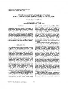
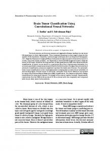
Fig. 1: the Architecture of Elastic network

and without auxiliary outputs Inception models, respectively. Experimental results showed that in the case with auxiliary outputs, classification accuracy was improved by 0.4% in top-1 accuracy than the case without adapting intermediate outputs. In addition to regularization, intermediate outputs are also expected to enhance the convergence during neural networks training. Deeply-supervised Nets (DSN) [14] connected support vector machine (SVM) classifiers after the individual hidden layers. Authors declared that the intermediate classifiers promote more stable performance and improve convergence ability during training. More recently, many studies related to a more systematic approach of using intermediate outputs with neural networks have appeared. In Teerapittayanon et al. [9], two extra intermediate outputs were inserted to AlexNet. This was shown to improve the accuracy on both the last and early outputs. The advantages of introducing auxiliary outputs has also been studied in Yong et al. [8], where the authors compare different strategies for gradient propagation (for example, should the gradient from each output be propagated separately or jointly). Moreover, our recent work [10] studied the same idea for regression problems mainly from the computational performance perspective. Here, we extend that work to classification problems and concentrate mainly on accuracy improvement instead of computational speed. III. P ROPOSED A RCHITECTURE A. Attaching the intermediate outputs In the structure of the intermediate outputs shown in Fig. 1, each unit of intermediate outputs consists of a global average pooling layer, a dropout layer, a fully connected layer and a classification layer with softmax function. The insight behind the global average pooling layer is that generally the data size at the early layers is large (e.g., 224 × 224 × 3), and attaching a fully connected layer directly would introduce an unnecessarily large number of new parameters.

… 56x56x64

Conv_depthwise

1x1x100

Fully connected 114x114x64 1x1x64

Conv_padding

112x112 Global average pooling 112x112x64

Pointwise relu

Fig. 2: The intermediate output on the top of the first “depthconv” block in MobileNet on CIFAR 100 The same intermediate output structure is directly connected to the network after each convolutional unit. B. The number of outputs and their positions Since network learns low level features on the early layers, the total number of weights allocated to the intermediate outputs is crucial to the final result. The number and the position of intermediate outputs in Elastic Nets are separately designed based on the different original network structures (e.g. network depth, network width). Although our general principle is to add auxiliary outputs after every layer, the particular design of the widely used networks require some adjustment. The network specific adjustments for each network in our experimentation are described next. Elastic-Inception V3 is based on the Inception-V3 architecture [13] having 94 convolutional layers arranged in 11 Inception blocks. We add intermediate outputs after the “concatenate” operation in each Inception block except the last one. Together with the final layer, in total, there are 11 outputs in the resulting Elastic-Inception V3 model. Elastic-DenseNet-121 is based on the DenseNet-121 architecture [16] with the growth rate hyperparameter equal to 32. DenseNet-121 consists of 121 convolutional layers

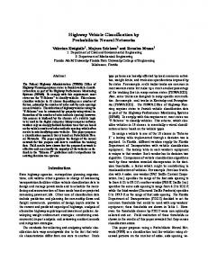
TABLE I: Testing error rate (%) on CIFAR 10 and CIFAR 100. Model

1

w/o Elastic Structure DenseNet-121 6.35 DenseNet-169 8.14 6.39 Inception V3 MobileNet 10.37 VGG-16 7.71 ResNet-50 5.54 ResNet-50-5 5.54 PyramdNet + ShakeDrop2 2.3 1 All the models we use are pretraiend on ImageNet 2 the state of the art accuracy [15]

CIFAR-10 w/ Elastic Structure 5.44 5.58 4.48 7.82 8.20 6.19 5.39 -

grouped into 4 dense blocks and 3 transition blocks. We attach each intermediate output after the “average pooling” layer of each transition block. We apply the same strategy for building Elastic-DenseNet-169, where the backbone is similar but deeper than the DenseNet-121. Totally, there are 4 outputs in both Elastic-DenseNet-121 and Elastic-DenseNet-169. Elastic-MobileNet is based on the MobileNet architecture [7] with hyperparameters α = 1 and ρ = 1. Here, an intermediate output is added after the “relu” activation function in each depthwise convolutional block. MobileNet has 28 convolutional layers and consists of 13 depthwise convolutional blocks. Elastic-MobileNet has 12 intermediate outputs besides 1 final classifier. We illustrate a part of the intermediate output structure from Elastic-MobileNet in Fig 2. Elastic-VGG-16 design is based on VGG16 architecture [3]. Intermediate outputs are attached after each of the “maxpooling” layers. In total, there are 5 outputs in Elastic-VGG16. Elastic-ResNet-50 is designed based on ResNet50 [4]. Intermediate outputs are attached after each of the “add” operation layers in the identity block and the conv block. The conv block is a block that has a convolutional layer at shortcut, identity block is a block with no convolutional layer at shortcut. In total, there are 16 total outputs in ElasticResNet-50. C. Loss function and weight updates Forward and backpropagation are executed in a loop during the training process. In the forward step, denote the predicted ˆ (i) = result at intermediate output i ∈ {1, 2, . . . , N } by y (i) (i) (i) [ˆ y1 , yˆ2 , . . . , yˆC ], where C is the number of classes. We assume that the output yields from the softmax function:   (k) exp zi (i)  , (1) yˆk = softmax(z) = X (c) exp zi c∈{1,...,C}

where z is a vector output of the last layer before the softmax. As shown in Fig. 1, loss functions are connected after softmax function. Denote the negative log-loss at i’th intermediate output by X 1 Li (ˆ y(i) , y(i) ) = − yc(i) log yˆc(i) , (2) C c∈{1,...,C}

Improvement 14.3% 31.5% 29.9% 24.6% -6.4% -11.7% 2.7% -

w/o Elastic Structure 24.48 23.06 24.98 38.60 38.06 21.96 21.96 12.19

CIFAR-100 w/ Elastic Structure 23.44 21.65 21.83 25.22 33.03 24.20 21.54 -

Improvement 4.3% 6.1% 12.6% 34.7% 13.2% -10.2% 1.9% -

where y(i) is the one hot ground truth label vector at output (i) i, and yˆc is the predicted label vector on the i’th output. The final loss function Ltotal is the weighted sum of losses at the intermediate outputs: Ltotal =

N X

  ˆ (i) , y(i) , w i Li y

(3)

i=1

with weights wi adjusting the relative importance of individual outputs. In our experiments, we set wi = 1 for all i ∈ {1, . . . , N }. IV. E XPERIMENTS We test our framework on the commonly used CIFAR10 and CIFAR100 datasets [17]. Both of them are composed of 32×32 color images. CIFAR10 has 10 exclusive classes, and there are 50,000 and 10,000 images in training and testing sets, respectively. CIFAR100 contains 100 classes, and each class has 500 training samples and 100 testing samples. A. Experimental setup and training At network input, the images are resized to 224×224×3 and we normalize the pixels to the range [0,1]. Data augmentation is not used in our experiment. We construct Elastic Nets using Keras platform [18]. The weights for different Elastic Nets are initialized according to their original networks pretrained on ImageNet, except the output layers that are initialized at random. Since we introduce a significant number of random layers at the network outputs, there is a possibility that they will distort the gradients leading into unstable training. Therefore, we first train only the new random layers with the rest of the network frozen to the imagenet-pretrained weights. This is done for 10 epochs with a constant learning rate 10−3 . After stabilizing the random layers, we unfreeze and train all weights with an initial learning rate 10−3 for 100 epochs. Learning rate is divided by 10 after the decaying loss on validation set staying on plateau for 10 epochs. All models are trained using SGD with mini-batch size 16 and a momentum parameter 0.9. The corresponding original networks are trained with the same settings. Moreover, data augmentation is omitted, and the remaining hyperparameters are chosen according to the library defaults [18].

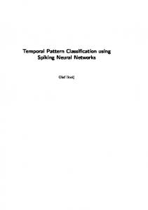
TABLE II: Testing error rate (%) of Elastic-DenseNet-169 with 4 different depth models, DenseNet-169 and DenseNet121 on CIFAR 100. Model Elastic-DenseNet-169-output-14 Elastic-DenseNet-169-output-39 Elastic-DenseNet-169-output-104 Elastic-DenseNet-169-output-168 DenseNet-169 DenseNet-121

# conv layer 14 39 104 168 168 120

params 0.39M 1.47M 6.71M 20.90M 20.80M 12.06M

error 73.37 48.96 22.86 21.65 23.06 24.48

B. Results In our experiment, we wish to compare the effect of intermediate outputs with their corresponding original nets. In our framework, each intermediate output can be used for prediction. For convenience, we only compare the last layer output as it is likely to be the most accurate prediction. The results on CIFAR test datasets are shown in Table I. From Table I we can see that in general the Elastic structured networks perform better compared to most of their backbone architectures for both datasets. More specifically, the use of intermediate outputs and their respective losses improves the accuracy for all networks except VGG-16 and ResNet50 for both datasets. Moreover, for CIFAR-100, ResNet-50 is the only network that does not gain in accuracy from the intermediate outputs. In CIFAR100, Elastic-DenseNet-169 achieves the lowest error rate (5.58%) among all models, which is 6.1% lower error rate than DenseNet-169. Elastic-DenseNet-121 and ElasticInception V3 have the better result than the original models as well, which reduce the error rate by 4.3% and 12.6% respectively. In CIFAR 10, Elastic-DenseNet-169 decreases 31.5% error compared to DenseNet-169. Elastic-DenseNet-121 and Elastic-Inception V3 outperform the back-bone networks by 14.3% and 29.9%. In relative terms, the highest gain in accuracy is obtained with MobileNet. Namely, Elastic-MobileNet achieves testing error of 25.22%, exceeding the backbone MobileNet (38.60%) by 35% relative improvement in CIFAR 100, and it’s the biggest performance improvement compared to all other Elastic Nets. In CIFAR 10, Elastic-MobileNet also reduces the error by 25%. There are two exceptions to the general trend: VGG16 and ResNet50 are not always improving in accuracy with the intermediate outputs. One possible reason is that VGG is shallow convolutional neural network. There is less gradient vanishing issue (over-parameters). Therefore, adding intermediate outputs effect positively less. The same reason probably holds for the ResNet-50 architecture, as well. Although the network itself is deep, there are shortcut connections every few layers, which help to propagate the gradient more effectively. Due to these reasons, the added layers do not have equally significant improvement as with the other networks. Additionally, the number of intermediate outputs is clearly the highest with the ResNet-50. In order to verify whether this might be a part of the reasons why ResNet-50 does not gain from our methodology, we decreased their number from 17 to

4 by removing all but the 2nd, 6th, 9th, and 12th intermediate outputs. This structure is denoted as ”Elastic-ResNet-50-5” in Table I. In this case, Elastic-ResNet-50-5 outpeforms the original ResNet-50 slightly by decreasing error by 2.7% and 1.9% on CIFAR 10 and CIFAR 100, respecively. So far, we have concentrated only on the accuracy of the last layer of the network. However, the accuracy of the intermediate layers is also an interesting question. In our earlier work [10] we have discovered that also the other late layers are relatively accurate in regression tasks. Let us now study this topic with one of the experimented networks. We study the case of DenseNet-169, because it has fewer intermediate outputs than the others and is thus easier to understand. The Elastic extension of this network has three intermediate outputs (after layers 14, 39 and 104) and the final output (after layer 168). We compare the Elastic extension of DenseNet-169 against the normal DenseNet-169 in Table II. The errors of all four outputs for test data on CIFAR 100 are shown on the rightmost columns and show that the best accuracy indeed occurs when predict from the ultimate layer. On the other hand, also the penultimate layer is more accurate than the vanilla DenseNet, and has remarkably fewer parameters. Moreover, using the 104’th layer output of the DenseNet turns out to be also more accurate than DenseNet121, which is roughly the same depth but with significantly more parameters. V. D ISCUSSION AND CONCLUSION This paper investigates employing intermediate outputs while training deep convolutional networks. When neural networks become to deeper, the gradient vanishing and overfitting problems result in decreasing classification accuracy. To mitigate these issues, we proposed to feed the gradient directly to the lower layers. In the experimental section we showed that this yields significant accuracy improvement for many networks. There may be several explanations for this behavior, but avoiding the vanishing gradient seems most plausible, since the residual networks with shortcut connections do not gain from the intermediate outputs. Interestingly, we also discovered, that using early exits from deep networks can be more accurate than the final exit of a network of equivalent depth. In particular, we demonstrated that using the 104’th exit of the DenseNet-169 becomes more accurate than the full DenseNet-121 when trained with the proposed framework. R EFERENCES [1] O. Russakovsky, J. Deng, H. Su, J. Krause, S. Satheesh, S. Ma, Z. Huang, A. Karpathy, A. Khosla, M. Bernstein et al., “Imagenet large scale visual recognition challenge,” International Journal of Computer Vision, vol. 115, no. 3, pp. 211–252, 2015. [2] A. Krizhevsky, I. Sutskever, and G. E. Hinton, “Imagenet classification with deep convolutional neural networks,” in Advances in neural information processing systems, 2012, pp. 1097–1105. [3] K. Simonyan and A. Zisserman, “Very deep convolutional networks for large-scale image recognition,” arXiv preprint arXiv:1409.1556, 2014. [4] K. He, X. Zhang, S. Ren, and J. Sun, “Deep residual learning for image recognition,” in Proceedings of the IEEE conference on computer vision and pattern recognition, 2016, pp. 770–778.

[5] V. Nair and G. E. Hinton, “Rectified linear units improve restricted boltzmann machines,” in Proceedings of the 27th international conference on machine learning (ICML-10), 2010, pp. 807–814. [6] S. Ioffe and C. Szegedy, “Batch normalization: Accelerating deep network training by reducing internal covariate shift,” arXiv preprint arXiv:1502.03167, 2015. [7] A. G. Howard, M. Zhu, B. Chen, D. Kalenichenko, W. Wang, T. Weyand, M. Andreetto, and H. Adam, “Mobilenets: Efficient convolutional neural networks for mobile vision applications,” arXiv preprint arXiv:1704.04861, 2017. [8] Y. Guo, M. Tan, Q. Wu, J. Chen, A. V. D. Hengel, and Q. Shi, “The shallow end: Empowering shallower deep-convolutional networks through auxiliary outputs,” arXiv preprint arXiv:1611.01773, 2016. [9] S. Teerapittayanon, B. McDanel, and H. Kung, “Branchynet: Fast inference via early exiting from deep neural networks,” in Pattern Recognition (ICPR), 2016 23rd International Conference on. IEEE, 2016, pp. 2464–2469. [10] Y. Bai, S. S. Bhattacharyya, A. P. Happonen, and H. Huttunen, “Elastic neural networks: A scalable framework for embedded computer vision,” arXiv preprint arXiv:1807.00453, 2018. [11] N. Srivastava, G. Hinton, A. Krizhevsky, I. Sutskever, and R. Salakhutdinov, “Dropout: a simple way to prevent neural networks from overfitting,” The Journal of Machine Learning Research, vol. 15, no. 1, pp. 1929–1958, 2014. [12] C. Szegedy, W. Liu, Y. Jia, P. Sermanet, S. Reed, D. Anguelov, D. Erhan, V. Vanhoucke, and A. Rabinovich, “Going deeper with convolutions,” in Proceedings of the IEEE conference on computer vision and pattern recognition, 2015, pp. 1–9. [13] C. Szegedy, V. Vanhoucke, S. Ioffe, J. Shlens, and Z. Wojna, “Rethinking the inception architecture for computer vision,” in Proceedings of the IEEE conference on computer vision and pattern recognition, 2016, pp. 2818–2826. [14] C.-Y. Lee, S. Xie, P. Gallagher, Z. Zhang, and Z. Tu, “Deeply-supervised nets,” in Artificial Intelligence and Statistics, 2015, pp. 562–570. [15] Y. Yamada, M. Iwamura, and K. Kise, “Shakedrop regularization,” arXiv preprint arXiv:1802.02375, 2018. [16] G. Huang, Z. Liu, L. Van Der Maaten, and K. Q. Weinberger, “Densely connected convolutional networks.” in CVPR, vol. 1, no. 2, 2017, p. 3. [17] A. Krizhevsky and G. Hinton, “Learning multiple layers of features from tiny images,” Citeseer, Tech. Rep., 2009. [18] F. Chollet et al., “Keras,” https://github.com/fchollet/keras, 2015.