Electric vehicle energy consumption modelling and prediction ... - MDPI

World Electric Vehicle Journal Vol. 7 - ISSN 2032-6653 - ©2015 WEVA

Page WEVJ7-0447

EVS28 KINTEX, Korea, May 3-6, 2015

Electric vehicle energy consumption modelling and prediction based on road information Jiquan Wang1, Igo Besselink1, Henk Nijmeijer1 1

Dynamics and Control Group, Department of Mechanical Engineering, Eindhoven University of Technology, Den Dolech 2, 5612 AZ Eindhoven, the Netherlands

Abstract The limited driving range is considered as a significant barrier to the spread of electric vehicles. One effective method to reduce “range anxiety” is to offer accurate information to the driver on the remaining driving range. However, the energy consumption during driving is largely determined by driving behaviour, road topography information and traffic situation, which are hard to predict. This paper will discuss an accurate electric vehicle energy consumption model validated using driving tests on different public roads, and then the model is used to predict future energy consumption based on road information. The energy consumption model includes five parts: the road load model, the powertrain loss model, the regenerative braking model, the auxiliary system model and the battery model. The parameters of these models are obtained through driving tests on public road and dynamometer tests in the TU/e Automotive Engineering Science lab. The results show that the model can calculate the energy consumption with a maximum error of 5% based on driving speed under different circumstances. To predict the future energy consumption, the road information is obtained from OpenStreetMap and Shuttle Radar Topography Mission. An offline algorithm is built to predict the energy consumption for a future trip based on the road information. The algorithm gives two energy consumption results: one is for the fastest driving speed; the other one is for the most economic driving speed. The results show that the measured energy consumption results for different types of road driving are all within the algorithm’s prediction scope. Therefore, the offline algorithm can give an accurate energy consumption estimation to the driver before a trip begins. Keywords: Electric vehicle, Energy consumption model, Road information, Energy prediction

1 Introduction Electric vehicles (EVs) are considered as future cars to solve oil dependency and environmental problems. However, the spread of EVs is limited by high price, long charging time, few charging stations and limited driving range. The limited driving range and long charging time may lead to

“range anxiety”, which can be explained as the drivers’ concern of not reaching the destination during driving [1]. Range anxiety is considered as one of the major factors that affect the acceptance of electric vehicles. Apart from a bigger battery, an accurate range estimation system is necessary to solve range anxiety. However, the prediction of the remaining range is complicated, because it is dependent on

EVS28 International Electric Vehicle Symposium and Exhibition

1


some stochastic factors such as vehicle characteristics, driving behaviour, traffic state, road topography and weather condition. Several studies have been performed to predict the remaining driving range of EVs. They mainly focus on predicting the driving speed [2-4] and obtaining the traffic information and road topography information [5-7]. The predicted driving speed and road information can help to improve the prediction accuracy. However, there are still two problems that need to be solved. Firstly, the energy consumption is also determined by the vehicle characteristic parameters, and some of the vehicle parameters are influenced by the weather condition and driving behaviour. Secondly, the driving speed may be difficult to predict accurately before a trip begins, because the driving speed is influenced by the traffic flow. In this paper, an offline algorithm is developed to solve these two problems. The algorithm can give the driver a first view on the energy consumption for a future trip based on different driving speed predictions including considering the weather influence. This research is based on an electric vehicle: TU/e Lupo EL. The TU/e Lupo EL is built from a donor vehicle VW Lupo 3L by the Dynamics and Control group of Eindhoven University of Technology in 2009, where EL is the abbreviation of “Electric Lightweight”. The TU/e Lupo EL is allowed to drive on the public road since spring 2011 [8-9].

Page WEVJ7-0448

driving tests, including highway driving, city driving and rural driving are shown to verify the offline algorithm.

2 Energy consumption model The energy flow of an electric vehicle for driving is shown in Figure 2. The electric energy is taken from the battery: a small part is used for the auxiliary system; the main energy is transformed by the electric motor into mechanical energy, which is used to overcome the road load. The electric vehicle energy consumption model is built in a backward way in this research. This means that the vehicle driving speed is the model input and the battery energy is the model output. The energy consumption model can be divided into five parts from the vehicle wheel to the battery: the road load model, the powertrain loss model, the regenerative braking model, the auxiliary system model and the battery model. The auxiliary system components energy consumption can be measured, the results are reported in [9]. The battery model adopted is a simple battery equivalent circuit model [10]. This paper will mainly introduce the road load model, the powertrain loss model and the regenerative braking model. The parameters of those models are obtained from different tests. Auxiliary system drive shaft 80 % of nominal capacity

Inverter motor

reduction

battery Discharging

wheel

Figure 2: Energy flow of an electric vehicle

2.1

Road load model

The moving of a vehicle on a road is influenced by the road load, which includes rolling resistance 𝐹𝑟 , aerodynamic drag force 𝐹𝑎𝑖𝑟 , road slope force 𝐹𝑔 and acceleration force 𝐹𝑖 , as shown in Figure 3. Figure 1: Lupo 3L with the existing diesel and new electric powertrain

This paper is organized as follows. In section 2, an energy consumption model is built with considering the influence of the weather condition based on the measurement data. In section 3, the road information is obtained from the OpenStreetMap (OSM) and Shuttle Radar Topography Mission (SRTM). Then the energy consumption for a future trip is predicted based on the road information. In section 4, three

Figure 3: Outside forces acting on a driving vehicle


2


where 𝐹𝑥 is the propelling force, 𝐹𝑟 is the rolling resistance force, 𝐹𝑎𝑖𝑟 is the air dynamic drag force, 𝐹𝑔 is the gravity force, 𝐹𝑖 is the acceleration force caused by vehicle inertia, 𝑓𝑟 is the rolling resistance coefficient, 𝑚 is the vehicle mass, 𝑔 is the gravitational acceleration, 𝜌 is the air density, 𝐶𝑑 is the aerodynamic drag coefficient, 𝐴 is the vehicle frontal area, 𝑣 is the vehicle speed, 𝑤 is the wind speed in the vehicle driving direction, 𝛼 is the road slope, 𝑚𝑒𝑓𝑓 is the vehicle effective mass, 𝑎𝑥 is the vehicle acceleration. The vehicle effective mass 𝑚𝑒𝑓𝑓 is the sum of the vehicle mass and the equivalent mass of the motor and wheel inertia. 4 ∙ 𝐽𝑤 𝐽𝑒𝑚 𝑚𝑒𝑓𝑓 = 𝑚 + 2 + 2 2 (2) 𝑅𝑒 𝑟𝑑 ∙ 𝑅𝑒

slope can be calculated based on the road information. However, the air density 𝜌 is changing with the weather condition, and the rolling resistance coefficient 𝑓𝑟 is determined by the weather and road condition. Therefore, these two parameters are always changing at different driving conditions. To model the energy consumption, the changing trend of these two parameters should be identified. 2.1.1 Air density The air density is a function of pressure, relative humidity and ambient temperature, while the humidity has a minor influence on the air density at higher temperature [12]. According to the equations published in [12], the value of air density is shown in Figure 4 for the condition that the humidity equals 80%. As can be seen, the air density will decrease with a temperature increase and air pressure decrease. Air density, 80% humidity 1.5

1.4

where 𝑚 is the vehicle mass, 𝐽𝑤 is the wheel inertia, 𝐽𝑒𝑚 is the motor inertia, 𝑅𝑒 is the tyre effective rolling radius and 𝑟𝑑 is the gear reduction ratio.

𝑓𝑟 𝜃 𝑎 𝑣 𝑤

Dependency

Variability

-

Stable

Passengers Weather Road Weather Weather Traffic Road Driver Weather route

Low High

Extremely high

All the parameters in Equation (1) need to be determined to build the road load model. Since the variability properties of these parameters are different (see Table 1), those parameters can be determined separately. The stable parameters can be obtained by doing tests in a lab. The extremely high variability parameters can be measured during the driving. The vehicle mass is dependent on the passengers number. The road

1.35 1.3 1.25 1.2 1.15

Table 1: Variability of vehicle longitudinal dynamics equation parameters Parameters 𝑔 𝐶𝑑 𝐴 𝑚 𝜌

1050 hPa 1025 hPa 1000 hPa 975 hPa 950 hPa

1.45

Air density [kg/m3]

The vehicle’s longitudinal dynamic equation is: 𝐹𝑥 = 𝐹𝑟 + 𝐹𝑎𝑖𝑟 + 𝐹𝑔 + 𝐹𝑖 1 (1) = 𝑓𝑟 ∙ 𝑚 ∙ 𝑔 + ∙ 𝜌 ∙ 𝐶𝑑 ∙ 𝐴 ∙ (𝑣 − 𝑤)2 2 +𝑚 ∙ 𝑔 ∙ sin 𝛼 + 𝑚𝑒𝑓𝑓 ∙ 𝑎𝑥

Page WEVJ7-0449

1.1 1.05

-20

-10

0 10 Ambient temperature [deg.C]

20

30

Figure 4: Air density as a function of ambient temperature and pressure [12]

2.1.2 Rolling resistance coefficient A series of coast down tests have been performed to obtain the rolling resistance coefficient at different conditions. During a coast down test, the propulsion is removed when the vehicle reaches a certain speed, and then the road load, consisting of rolling resistance, aerodynamic drag and friction force, will slow down the vehicle until the vehicle comes to a standstill. The differential equation describing the longitudinal dynamics in a coast down test is given as 𝑚𝑒𝑓𝑓 ∙ 𝑣̇ = −𝑓𝑟 ∙ 𝑚 ∙ 𝑔 𝑇𝑓𝑟 1 (3) − ∙ 𝜌 ∙ 𝐶𝑑 ∙ 𝐴 ∙ (𝑣 − 𝑤)2 − 2 𝑅𝑒 where 𝑇𝑓𝑟 is the friction moment in the gearbox and wheel bearings. The rolling resistance coefficient is dependent on the road surface, ambient temperature and driving speed [13]. Different coast down tests are done to


3


obtain the relation between the rolling resistance coefficient with these factors. A comparison between simulation and measurement of the coast down tests on different road types in summer are shown in Figure 5. Through the comparison, the value of rolling resistance coefficient can be obtained. The rolling resistance on a highway road (smooth asphalt) is 0.0095 and it increases to 0.0157 on a coarse rural road (Rijtvenweg test); the increase is about 65%. It can be seen that the difference is really significant. However, it is difficult to obtain the rolling resistance coefficient on every road section. This relative difference between highway road and rural road will be used to estimate the relative relationship of rolling resistance coefficient on other types of road, and the result is shown in Table 3. Rijtven test 1 Rijtven test 2 Simulation frr=0.0157 Highway test 1 Highway test 2 Simulation frr=0.0095

100

80

Velocity [km/h]

The effect of temperature on rolling resistance is shown in Figure 6. A comparison of simulation and measurement of coast down tests on a highway road in summer and winter is shown in Figure 6. The summer test was done on 1st August 2013, the ambient temperature was about 29 degree Celsius, and 𝑓𝑟 was then determined to be 0.0095. The winter test was done on 11th December 2013, the ambient temperature was about 2.5 degree Celsius, and 𝑓𝑟 was then determined to be 0.0132. The increase of 𝑓𝑟 is 39% from 29 ºC to 2.5 ºC. Based on the measurement data at different temperatures, the relationship between the rolling resistance coefficient with the temperature is given in Equation 5. 2 𝑓𝑟0 = 1.9 × 10−6 ∙ 𝑇𝑎𝑚𝑏 − 2.1 × 10−4 (5) ∙ 𝑇𝑎𝑚𝑏 + 0.013

2.2

120

60

40

20

0

Page WEVJ7-0450

0

50

100 Time [s]

150

200

Powertrain loss model

The vehicle powertrain components consist of a MES-DEA TIM 600 inverter, a MES-DEA A200200W water cooled AC induction motor and a Carraro reduction gear/differential (gear ratio 1:8.654). To determine the power loss, a test was executed on a dynamometer in the TU/e AES lab. The experiment is shown in Figure 7 [14]. The vehicle’s front wheels are put on the dynamometer in the test.

Figure 5: Coast down test on highway road and rural road

Apart from the road surface, the rolling resistance coefficient is influenced by the weather and the driving speed. Therefore, the rolling resistance coefficient can be expressed as (4) 𝑓𝑟 (𝑇𝑎𝑚𝑏 , 𝑣) = 𝑓𝑟0 (𝑇𝑎𝑚𝑏 ) + 𝑓𝑟1 ∙ 𝑣 where 𝑇𝑎𝑚𝑏 is the ambient temperature, 𝑓𝑟1 is a constant value 5.4 × 10−5, and 𝑓𝑟0 is determined by experiments. 120 summer test 1 summer test 2 simulation frr=0.0095 winter test 1 winter test 2 simulation frr=0.0132

100

Velocity [km/h]

80

60

40

20

0

0

50

100 Time [s]

150

200

Figure 6: Coast down test on highway road at different time

Figure 7: Dynamometer test in AES lab

When the drum is running at a constant speed, the output of the motor is changed by changing the inverter control signal. When the inverter control signal is bigger than 50, the vehicle is in traction mode, and the vehicle is in regenerative braking mode when the inverter control signal is smaller than 50. The motor electric power and bench mechanical power can be measured during the experiment, as illustrated by Figure 8. It can be seen from Figure 8, when the inverter control signal is 50, the motor is idling, the efficiency is zero, but the power loss still exists because of the friction. Therefore, the power loss is used to


4


Figure 8: The method of calculating the powertrain loss

The powertrain loss at a specific speed is the difference between the motor electric power and drum mechanical power. After processing the measurements, the relationship between the power loss and motor mechanical torque at different driving speed is shown in Figure 9. As can be seen, the power loss is different for the traction part and regenerative braking part at the same motor mechanical power.

For the regenerative mode, the empirical equation is: (7) 𝑃𝑙𝑜𝑠𝑠 = 0.21 ∙ 𝑇 2 + 0.097 ∙ |𝑇| ∙ 𝜔 + 𝑃𝑐 where 𝑇 is the motor torque, 𝜔is the motor angular speed, 𝑃𝑐 is the motor idling power loss. The power loss difference between the calculation and the measurement is depicted in Figure 10. It can be seen that the error is smaller than 0.5 kW in most cases. Therefore, the empirical equations are sufficiently accurate and can be used to calculate the powertrain loss. Based on the equations, the powertrain efficiency map is calculated and depicted in Figure 11. It can be seen that the powertrain efficiency is better in the traction mode than in the regenerative braking mode at the same motor output. 6.2 km/h 12.4 24.8 37.2 49.7 62.1 74.5 86.9 99.3 111.8 124.2

2

1.5

Power loss difference [kW]

represent the powertrain energy loss instead of efficiency map.

Page WEVJ7-0451

1

0.5

0

-0.5

6.2 km/h 12.4 24.8 37.2 49.7 62.1 74.5 86.9 99.3 111.8 124.2

Power loss [kW]

10

8

6

-40

-30

-20

-10 0 10 Mechanical power [kW]

20

30

40

Figure 10: The powertrain loss difference between simulation and measurement 0.9

250

0.3 0.3

0.20.4 0.4 200 0.2

4

0.8 0.6 0.6

150 2

-40

-30

-20 -10 0 10 20 Motor mechanical power [kW ]

30

Torque [Nm]

0 -50

40

0.85 0.85

50

0.92

0.6

0.92

0.5 0.85 0.85

-50

0.4

0.80.8 0.6 0.6

-150

0.3

0.70.7 0.5 0.1 0.10.5

-200

To simplify the calculation, algebraic equations are used to describe the power loss. Since the power loss for the traction mode and regenerative mode are different, separate empirical equations are used to calculate the power loss. Most of the power loss is caused by the inverter and motor, thus, the power loss can be calculated based on the motor torque and angular speed. The MATLAB/Simulink Parameter Estimation Tool is used to get the empirical equation structure and optimize the value of parameters. For the traction mode, the empirical equation is: 𝑃𝑙𝑜𝑠𝑠 = 0.3158 ∙ 𝑇 2 + (2.2 × 10−10 ∙ 𝜔3 (6) −1.62 × 10−7 ∙ 𝜔2 + 3.44 × 10−5 ∙ 𝜔) ∙ 𝑇 3 + 𝑃𝑐

0.9 0.9

0

-100

Figure 9: The relationship between the powertrain loss and the motor mechanical power at different speeds

0.7

0.7 0.7 0.80.8

100

0.2

0.4 0.4

-250 0

200

400 600 800 Angular Velocity [rad/sec]

1000

0.1

Figure 11: The powertrain efficiency map

2.3

Regenerative braking model

There are two kind of regenerative braking control strategies in the Lupo EL. The first one is a parallel regenerative braking control strategy, the other one is a one pedal driving control strategy. 2.3.1

Parallel regenerative braking control strategy The parallel regenerative braking control strategy in the Lupo EL is based on the brake pedal travel.


5


60 km/h 10000

Brake force [N]

8000

Total brake force Regenerative force

6000 4000

5 accelerator pedal released brake pedal actuation accelerator pedal > 30%

4 3 2

Acceleration [m/s ]

The total braking force and regenerative braking force are shown in Figure 12 when the driving speed is 60 km/h. As can be seen, when the brake pedal travel is below 10%, the hydraulic braking force is zero, this is the free travel between the brake disc and brake drum. And when the brake pedal travel is bigger than 60%, the regenerative braking force is reduced to zero, which is to ensure the braking stability in an emergency case. However, there are two disadvantages in the parallel regenerative braking strategy. The first issue is that the braking force is not linear with the brake pedal travel, which may not provide a comfortable and consistent brake feel for the driver. The second issue is that the hydraulic braking system is always working during the braking, which results in part of the energy being transferred into heat. Therefore, the regenerative braking strategy needs to be modified to improve the braking feel and energy efficiency.

Page WEVJ7-0452

2 1 0 -1 -2 -3 -4

0

20

40

60 80 Driving speed [km/h]

100

120

Figure 13: One pedal driving control strategy

2.4

Driving verification

Some driving tests on public road are used to verify the energy consumption model. A total of twelve driving tests were recorded in 2013 and 2014. Six recordings, from May to November in 2013, are driven with the parallel regenerative braking algorithm. Another six recordings in 2014 are driven with the one pedal driving algorithm. The driving tests include constant speed driving, city driving and rural road driving. The battery output energy is measured during driving. The details of these tests and measured energy results are listed in Table 2. Table 2: The recording of driving tests on public road

2000

0 0

20

40 60 80 Brake pedal travel [%]

Date

Speed [km/h]

Distance [km]

May 6th May 7th Jun 17th Jun 5th Jun 6th Nov 27th Jun 6th Sep 2nd Jun 26th Dec 3rd Nov 15th Dec 2nd

80 100 120 City City City 95 115 City City Rural Rural

228.9 114.1 113.9 47.7 49.6 50.1 60.2 106.8 6.9 7.9 17.96 17.97

100

Figure 12: Parallel regenerative braking control strategy

2.3.2 One pedal driving control strategy A one pedal driving control strategy is designed to improve the performance of the vehicle. For the one pedal driving algorithm the maximum deceleration that can be achieved when releasing the accelerator pedal is increased to 2 m/s2. This allows the vehicle to be driven by the accelerator pedal alone in most cases, and the brake pedal is only applied for emergency cases. The relationship between forward speed and acceleration/deceleration in a driving test on the public road is shown in Figure 13. It can be seen that the driving test include the city driving and highway driving, and the brake pedal is seldom used during the test.

Parallel regenerative braking algorithm (2013) One pedal driving algorithm (2014)

DC energy [kWh] 22.6 16.6 18.4 5.1 5.3 6.8 6.7 15.6 0.7 1.0 1.9 2.1

The energy consumption of a driving test can be calculated using the energy consumption model based on the driving speed. Finally, the error of the model can be represented by the difference between the calculation and measurement: 𝐸𝑠𝑖𝑚𝑢𝑙𝑎𝑡𝑖𝑜𝑛 − 𝐸𝑚𝑒𝑎𝑠𝑢𝑟𝑒𝑚𝑒𝑛𝑡 (8) 𝑒= ∙ 100% 𝐸𝑚𝑒𝑎𝑠𝑢𝑟𝑒𝑚𝑒𝑛𝑡 The simulation results demonstrate that the energy consumption model can calculate the vehicle energy consumption based on the driving speed with an error smaller than 5% for different


6


circumstances. Therefore, the model is considered sufficiently accurate and can be used as a tool to predict the future energy consumption information to the driver.

Page WEVJ7-0453

speed is an empirical value based on the road type in this research. The structure of the offline algorithm is depicted in Figure 15.

Figure 15: The energy prediction offline algorithm structure

Figure 14: The difference between the simulation and measurement for energy consumption model

3.1

3 Energy consumption prediction To predict the energy consumption for a future trip, the road information, weather condition and driving speed should be known first, and then the energy consumption model can be used to calculate the required amount of energy. The road information, including route length, road slope, road direction and road type, can be obtained from OSM and SRTM. The ambient temperature, wind speed and direction can be obtained from the weather report. The driving speed is determined by the road type, traffic condition and driver behaviour. The driving behaviour varies from driver to driver and even may be different for the same driver at different time and situations. Therefore, the driving speed cannot be predicted accurately before a trip begins. However, the maximum driving speed and most economic driving speed can be obtained based on the road information to predict the energy consumption. The offline algorithm is designed to give a first estimation on the energy consumption to the driver before a trip begins. In the algorithm, two kinds of driving speed are determined: one is for the fastest driving, while the other one is for the most economic driving. Two energy consumption results are provided correspondent to the predicted driving speed. The fastest driving speed is determined by the speed limit based on road type. The most economic speed of the Lupo EL is about 25 km/h for constant speed driving [15], but this value will decrease while considering the influence of the frequently startand-stop driving in city route. Therefore, the most economic speed is set as the minimum driving speed on the road. The minimum driving

Road information

The road information for the future driving route, including the geographic coordinates, road type, traffic light position and speed limitation signs, can be obtained from the OpenStreetMap (OSM). OSM is a collaboration project to create a free editable map of the world that provides geographical data to anyone [16]. It is freely available and has no technical restrictions in terms of processing the data. The height information of the future route can be obtained from the Shuttle Radar Topography Mission (SRTM) based on the geographic coordinates. SRTM is an international research effort that obtained digital elevation models on a near-global scale from 56 degrees south to 60 degrees north latitude, which comprises almost 80% of Earth’s total landmass. The data has been released at two horizontal resolutions: 3 arcseconds (90 m) globally, and 1 arc-second (30 m) for the Unites States [17-18].

3.2

Driving speed

Four factors can be obtained from OSM to determine the vehicle driving speed: road type, speed limit sign, road curvature and traffic lights. The maximum driving speed and most economic driving speed are a combination effect of these four factors. 3.2.1 Road type Normally, there is a legal allowed driving speed scope for each type of road. Therefore, the first estimation of the maximum and most economic driving speed is determined by the road type. The relative rolling resistance on different road types have been estimated based on the coast down test results in Section 2.1.2.


7


2 𝑣𝑚𝑎𝑥 = 𝑎𝑦𝑚𝑎𝑥 𝑅

Table 3: Road type information based on OSM Road type footway pedestrian living street residential service track unclassified tertiary secondary primary trunk motorway

Page WEVJ7-0454

Type number

Maximum speed [km/h]

Minimum speed [km/h]

Relative rolling resistance

1

15

5

1.25

2 3 4 5 6 7 8 9 10

30 30 30 50 50 70 80 100 120

10 10 10 20 20 30 50 70 80

1.15 1.25 1.40 1.20 1.10 1.05 1.00 1.00 1.00

The maximum allowed speed is 130 km/h on about half of motorways in the Netherlands, while the value is 120 km/h on the other half [19]. However, normally the driver doesn’t drive at the maximum speed for long distance on motorway. Therefore, the maximum speed is set to 120 km/h for motorway driving. The results are shown in Table 3. 3.2.2 Speed limit sign The vehicle driving speed is also limited by the speed limit sign. The road speed limit sign is used in most countries to set the maximum (or minimum in some case) speed. Speed limit sign is normally indicated as a traffic sign in the street, as Figure 16 [20]. The speed limit sign is added as nodes information in OSM road information database, which can be investigated once the driving route is settled down.

(9)

where 𝑅 is the corner radius, 𝑣𝑚𝑎𝑥 is the maximum driving speed and 𝑎𝑦𝑚𝑎𝑥 is the maximum lateral acceleration. The maximum lateral acceleration can reach 8 m/s2 on a standard vehicle during driving [21], however, the maximum lateral acceleration is smaller than 4 m/s2 at most cases according to the Lupo EL driving test measurement. Therefore, the maximum lateral acceleration is considered as 4 m/s2 in this research. The road curvature can be calculated based on the coordinates obtained from OSM. 3.2.4 Traffic light The influence of traffic lights has to be considered, because the vehicle may have to stop and wait in front of a traffic light. However, whether the traffic light is red or nor, cannot be predicted offline. To obtain the average influence of traffic lights, half of traffic lights are assumed to be red, and the waiting time is estimated to be 20 s. The traffic lights are tagged to road nodes in OSM. The position of the traffic lights can be obtained once the future travel route has been determined. 3.2.5 Acceleration After combining the influence of the road type, speed limit sign, road curvature and traffic lights, the target speed for a specific route can be obtained. An illustration is shown in Figure 17. As can be seen, the target speed isn’t continuous, which cannot be realised by the vehicle. To obtain a realistic driving speed, the discontinuities between two target speed values should be connected by the vehicle acceleration and deceleration.

Figure 16: Speed limit sign in a street

3.2.3 Road curvature The vehicle maximum lateral acceleration will limit the driving speed if the steering radius is small in a corner. The relation between the maximum driving speed and maximum lateral acceleration is given as

Figure 17: Speed information from OSM

The maximum deceleration caused by regenerative braking and acceleration of Lupo EL are determined by the motor setting, the value can be


8


calculated by the vehicle longitudinal dynamic equation. The equation is given as 𝑃𝑚,𝑚𝑒𝑐ℎ 𝐹𝑟 + 𝐹𝑎𝑖𝑟 + 𝐹𝑔 (10) 𝑎𝑚𝑎𝑥 = − 𝑚∙𝑣 𝑚 The maximum motor electric power is set to 50 kW for traction and -24 kW for regenerative braking. The motor efficiency is set to a constant value 80% in this calculation. Therefore, when the motor efficiency is considered, the maximum motor mechanical power 𝑃𝑚,𝑚𝑒𝑐ℎ is 40 kW for traction and -30 kW for regenerative braking. The acceleration/deceleration is determined by the motor power setting at high driving speed, while it is limited by the tire-road friction coefficient at low speed driving. In this algorithm, the maximum acceleration and deceleration at low speed is determined by the driving tests measurement. The relationship between the acceleration/deceleration and driving speed in a driving test is shown in Figure 18. As can be seen, the maximum acceleration is set to 3 m/s2 and the maximum deceleration is set to 2 m/s2 at low speed driving.

Page WEVJ7-0455

The acceleration is used to connect the target speed into the realistic driving speed. The result is illustrated by the blue curve in Figure 17.

4 Results Several illustrative tests are shown in this section to verify the offline algorithm, including the highway driving, rural driving and city driving. The highway driving test illustrates how the offline algorithm works. City driving and rural driving are performed by four different drivers on the same routes. The results show that the algorithm can give an accurate energy prediction scope for different drives.

4.1

Highway driving

A highway driving test was done to verify the energy prediction algorithm on 2nd September 2014 from Eindhoven to Nijmegen. The route of the driving is shown in Figure 19. Wind direction 51.85

51.8

51.75

51.7

measurement measurement maximum acceleration maximum deceleration

4 3

2

Acceleration [m/s ]

Latitude [deg]

5

51.65

51.6

51.55

2

51.5

1

51.45

0

5.4

-1 -2

5.45

5.5

5.55

5.6 5.65 Longitude [deg]

5.7

5.75

5.8

5.85

5.9

Figure 19: Driving route from Eindhoven to Nijmegen

-3 -4

0

20

40

60 80 Speed [km/h]

100

120

140

Figure 18: The relation between the speed and acceleration/deceleration in a driving test

To determine the driving speed, road types along the route have to be obtained from OSM first, and the results are shown in Figure 20. Most part of the route is highway road, but other types of road are also included.

The acceleration during driving in this algorithm is determined by the difference between the current driving speed and target speed. If the difference is bigger than 10 km/h, the maximum acceleration is adopted, or else, the acceleration linearly decreases from the maximum acceleration to zero with the speed difference decrease. The equation is 𝑎𝑥,𝑚𝑎𝑥 , ∆𝑣 ≥ 10𝑘𝑚/ℎ (11) 𝑎𝑥 = { 𝑎𝑥,𝑚𝑎𝑥 ∙ ∆𝑣, ∆𝑣 < 10𝑘𝑚/ℎ 10

motorway trunk primary

Road type

secondary tertiary uncalssified track service residential

0

10

20 30 Distance [km]

40

50

Figure 20: Road type along the highway driving route

where 𝑎𝑥 is the current acceleration, 𝑎𝑥,𝑚𝑎𝑥 is the maximum acceleration at the current driving speed and ∆𝑣 is the difference between the current driving speed and target speed.

The height information along the driving route can be obtained from SRTM, and the result is shown in Figure 21. This again illustrate that the Netherlands is a very level country.


9


Page WEVJ7-0456

9 maximum speed minimum speed 90 km/h 100km/h 110 km/h Measurement

8

30

Energy consumption [kWh]

7

25

Height [m]

20

15

6 5 4 3 2

10

1 0

5

0

-1

0

10

20 30 Driving distance [km]

40

50

Figure 21: The height information along the highway driving route

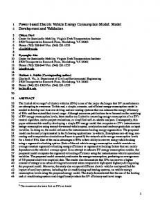
The speed information of simulation and measurement is shown in Figure 22. As can be seen, the highway driving speed can range from 80 km/h to 120 km/h. Normally, the driver needn’t to follow the traffic flow on highway road; he can choose his own driving speed. This will obviously affect the energy consumption results. To provide more energy consumption prediction information to the driver, more energy consumption results are calculated from 80 km/h to 120 km/h, the interval calculation speed is 10 km/h. The prediction and the measured energy consumption are shown in Figure 23. According to the measurement, most of the highway driving speed is between 110 km/h and 120 km/h, the measured energy consumption is also between the 110 km/h and 120 km/h driving speed energy prediction. This proves the accuracy of the algorithm on highway driving.

10


40

50

Figure 23: The simulation and measurement energy result along the highway driving route

4.2

City road driving

A driving route in the centre of Eindhoven is shown in Figure 24. The road type of the city driving route is shown in Figure 25. Four drivers have driven on this route, and the energy consumption results are recorded. The maximum and minimum predicted energy consumption results for this route are shown in Figure 26. As can be seen the measured energy consumption for four drivers are all between the minimum and maximum predicted result, which can confirm the accuracy of the approach. There are lots of traffic lights in the city route, thus the vehicle have to start-and-stop frequently. This is the reason why there are so many oscillations in the maximum driving speed energy consumption prediction result. 51.45 51.448 51.446 Latitude [deg]

140

120

100

Driving speed [km/h]

0

51.444 51.442 51.44 51.438

80

51.436 60

40

20

0

51.434 5.465

maximum speed minimum speed 90 km/h 100km/h 110 km/h Measurement 0

10


5.47


5.485

5.49

Figure 24: A driving route in Eindhoven centre 40

secondary

50

tertiary

Road type

Figure 22: The measurement and simulation driving speed along the highway driving route

unclassified

track

service

residential

0

1

2

3 Distance [km]

4

5

6

Figure 25: The road type in city centre driving


10


Page WEVJ7-0457

0.9

2.5 maximum speed minimum speed driver 1 driver 2 driver 3 driver 4


0.7 0.6

maximum speed minimum speed driver 1 driver 2 driver 3 driver 4

2


0.8

0.5 0.4 0.3 0.2

1.5

1

0.1

0.5 0 -0.1

0

1

2


5

6

0

Figure 26: The energy consumption in city centre driving

Rural road driving

4.3

A rural driving route in Eindhoven nearby is shown in Figure 27. The road type along this route can be seen in Figure 28. Four drivers have driven on this route and energy consumption results are recorded. The energy prediction results are shown in Figure 29. It is again shown that the energy consumption results are different for different drivers, but these four energy consumption results are all between the maximum and minimum energy prediction results. 51.5

Latitude [deg]

51.49 51.48 51.47 51.46 51.45 51.44 5.43

5.44

5.45

5.46


5.49

5.5

5.51

Figure 27: A rural driving route in Eindhoven primary

secondary

Road type

tertiary

unclassified

0

5

10 Driving distance [km]

15

20

Figure 29: The energy consumption in rural driving route

5 Conclusions The purpose of this work is to develop an offline algorithm for an electric vehicle range estimator, which can give a first impression to the driver on the possible energy consumption scope for a forthcoming trip. An energy consumption model is built based on measurements to predict the energy consumption. The model can calculate the energy consumption with a maximum error of 5% for different circumstances, which is accurate enough to be used in the offline algorithm. However, the rolling resistance coefficient varies significant on different road types, which need to be investigated further in future research. The model is used to predict the future energy consumption based on the road information obtained from OSM and SRTM. The highway driving, city driving and rural driving results show that the offline algorithm can provide an accurate energy consumption prediction scope for a future trip, which is suitable for different drivers. Additionally, the algorithm gives more prediction results based on different highway driving speeds, which can give a more precise advice when the driver is driving on highway road. The future work is to build an online algorithm for the range estimator. The purpose of the online algorithm is to adjust the energy prediction result during driving based on the driving behaviour.

track

Acknowledgments

service

residential

0

5

10 Distance [km]

15

20

Figure 28: The road type in rural driving route

The funding of PhD project of Jiquan Wang is provided by China Scholarship Council (CSC). Thanks to Vital van Reeven for providing the MATLAB tool to obtain data from OpenStreetMap. The authors would like to thank everyone involved in this project for their technical support and advice.


11


References [1]

Nilsson M., Electric Vehicle: The phenomenon of range anxiety, Lindholmen Science Park, Sweden, June 2011.

[2]

Hongwen He, et al., A method for identification of driving patterns in hybrid electric vehicles based on a LVQ neutral network, Energies, ISSN 1996-1073, 5 (2012), 3363-3380.

[3]

Valera J.J, et al., Driving cycle and road grade on-board predictions for the optimal energy management in EV-PHEVs, EVS27, 2013, Barcelona.

[4]

Frank A., et al., Drive cycle prediction and energy management optimization for hybrid hydraulic vehicles, IEEE Transaction on vehicular technology, ISSN 0018-9545, 62(2013), 3581-3592.

[5] Ravi Shankar, et al., Method for estimating the energy consumption of electric vehicles and plug-in hybrid electric vehicles under real-world driving conditions, IET Intelligent Transport System, ISSN 1751-956X, 7(2013), 138-150.

Page WEVJ7-0458

[15] I.J.M. Besselink, et al., Evaluating the TU/e Lupo EL BEV performance, EVS27, 2013, Barcelona. [16]

OpenStreetMap, http://en.wikipedia.org/wiki/ OpenStreetMap, accessed on 2014-12-17.

[17]

Shuttle Radar Topography Mission, http://en.wikipedia.org/wiki/shuttle_Radar_Topogr aphy_Mission, accessed on 2014-12-17.

[18] SRTM, http://wiki.openstreetmap.org/wiki/ SRTM, accessed on 2014-12-17. [19]

Speed limits in the Netherlands, http://en.wikipedia.org/wiki/Speed_limits_in_the_ Netherlands, accessed on 2015-01-21.

[20]

Speed limit, http://en.wikipedia.org/wiki/ Speed_limit, accessed on 2014-12-17.

[21] Gilles Reymond, et al., Role of lateral acceleration in curve driving: driver model and experiments on a real vehicle and a driving simulator, Human Factors, ISSN 0018-7208, 43(3): 483-495.

Authors

[6] Peter Ondruska, et al., Probabilistic attainability maps: efficiently predicting driver-specific electric vehicle range, IEEE Intelligent vehicles symposium (IV), 2014, Dearborn, Michigan, USA. [7]

Christophe Moure, et al., Range estimator for electric vehicles, EVS27, Barcelona, 2013.

[8]

I.J.M. Besselink, et al., Design of an efficient, low weight battery electric vehicle based on a VW Lupo 3L, EVS25, Shenzhen China, 2010.

[9]

P.F. van Oorschot, et al. Realization and control of the Lupo EL electric vehicle, EVS26, California USA, 2012.

[10] Jiquan Wang, et al. Evaluating and modeling the energy consumption of the TU/e Lupo EL BEV, Fisita 2014, Maastricht, the Netherlands. [11] Javier A. Oliva, et al., A model-based approach for predicting the remaining driving range in electric vehicles, Annual Conference of the Prognostics and Health Management Society 2013, New Orleans, USA.

Jiquan Wang is a PhD at the Eindhoven University of Technology, Department of Mechanical engineering, Dynamics and Control. Current research activities include electric vehicle energy modelling and driver support building. Dr. Ir. Igo Besselink is an assistant professor at the Eindhoven University of Technology, department of Mechanical engineering, Dynamics and Control. Research activities include tyre modelling, vehicle dynamics and electric vehicles. Prof. Dr. Henk Nijmeijer is a full professor at the Eindhoven University of Technology, department of Mechanical engineering, Dynamics and Control. Current research activities include non-linear dynamics and control.

[12] A. Picard, et al., Revised formula for the density of moist air (CIPM-2007), Metrologia, ISSN 0026-1394, 45(2008) 149-155. [13] Tony Sandberg, Heavy truck modeling for fuel consumption simulations and measurements, Linkoping University, thesis No. 924, Sweden. [14] Paul Kokke, et al., TU/e Lupo EL powertrain efficiency experiments, EEVC 2014, Brussels, Belgium.


12