Electrical Power Load Forecasting using Hybrid Self-Organizing ...

The 2ndInternational Power Engineering and Optimization Conference (PEOCO 2008), Shah Alam, Selangor, MALAYSIA. 4-5 June 2008.

Electrical Power Load Forecasting using Hybrid Self-Organizing Maps and Support Vector Machines J. Nagi, K. S. Yap S. K. Tiong, S. K. Ahmed, Member, IEEE

Abstract—Forecasting of future electricity demand is very important for decision making in power system operation and planning. In recent years, due to the privatization and deregulation of the power industry, accurate forecasting of future electricity demand has become an important research area for secure operation, management of modern power systems and electricity production in the power generation sector. This paper presents a novel approach for mid-term electricity load forecasting. It uses a hybrid artificial intelligence scheme based on self-organizing maps (SOMs) and support vector machines (SVMs). According to the similarity degree of time series input samples, the SOM is used as a filtering scheme to cluster historical electricity load data into two subsets using the Kohonen rule in an unsupervised manner. As a novel learning machine, the SVM based on statistical learning theory is used for prediction, using support vector regression (SVR). Two epsilon-SVRs are employed to fit the training data of each SOM clustered subset individually in a supervised manner for load prediction. The proposed hybrid SOM-SVR model is evaluated in MATLAB on the electricity load dataset used in the European Network on Intelligent Technologies (EUNITE) competition, arranged by the Eastern Slovakian Electricity Corporation. This proposed model is robust with different data types and can deal well with nonstationarity of load series. Practical application results show that this hybrid technique gives far better prediction accuracy for mid-term electricity load forecasting compared to previous research findings. Keywords—Support vector machine, self-organizing map, electrical power load forecasting, artificial intelligence.

L

I.

INTRODUCTION

OAD forecasting has always been a key instrument in power system operation. Many operational decisions in power systems, such as unit commitment, economic dispatch, automatic generation control, security assessment, maintenance scheduling, and energy commercialization depend on the future behavior of Jawad Nagi is with the Power Engineering Centre, Universiti Tenaga Nasional, 43009 Kajang, Malaysia (e-mail: [email protected]). Keem Siah Yap is with the Department of Electronic and Communication Engineering, Universiti Tenaga Nasional, 43009 Kajang, Malaysia. Email address: (e-mail: [email protected]). Sieh Kiong Tiong is with the Department of Electronic and Communication Engineering, Universiti Tenaga Nasional, 43009 Kajang, Malaysia (e-mail: [email protected]). Syed Khaleel Ahmed is with the Department of Electronic and Communication Engineering, Universiti Tenaga Nasional, 43009 Kajang, Malaysia (e-mail: [email protected]).

loads. In particular, with the rise of deregulation and free competition of the electric power industry all around the world, load forecasting has become more important than ever before. Load forecasts are currently being considered vital for energy transactions in competitive electricity markets[1]. In the recent years, accuracy of electricity load forecasting has received more attention on a regional and national scale. The error of electricity load forecasting may increase the cost of operation, where overestimation of the future load can result in excess supply. In contrast, underestimation of load leads to failure in providing enough electricity and implies high costs in peaking units[5]. During the last four decades, a wide variety of techniques have been used for the problem of load forecasting. Such a long experience in dealing with the load forecasting problem has revealed some time series modeling approaches based on artificial neural networks (ANNs) and statistical methods. Statistical models include moving average and exponential smoothing methods such as, multi-linear regression models, stochastic process, data mining approaches, autoregressive and moving averages (ARMA) models, Box-Jenkins methods, and Kalman filtering-based methods[1]. However, electric load time series are usually nonlinear functions of exogenous variables. Therefore, to incorporate non-linearity, ANNs have received much more attention in solving problems of electricity load forecasting. However, one major risk in using ANN models is the possibility of excessive training data approximation, i.e., overfitting, which usually increases the out-of-sample forecasting errors[4]. Hence, due to the empirical nature of ANN procedures their application is cumbersome and time consuming. Recently, new approaches based on machine learning techniques using support vector machines (SVMs) have been proposed for electricity load forecasting. Support vector regression (SVR) used in SVMs is a new and powerful machine learning technique for regression based analysis in statistical learning theory. SVRs established on the structure risk minimization principle (SRM) have shown to be very resistant to the overfitting problem of ANNs, by achieving a high generalization performance in solving forecasting problems of various time series[1]. Electricity demand now days is becoming difficult to forecast because of the variability of non-stationarity of load series that results from non-uniform demand supply, price-dependent loads, and time-varying prices. Therefore, more sophisticated forecasting tools with higher accuracy are required for modern power systems. This paper focuses on mid-term electricity load forecasting to predict the month-ahead electricity load profile, using historical electricity data from the 2001 51

EUNITE competition[7] with a time series modeling approach. The EUNITE competition data is an internetbased dataset and has been employed to allow reproduction of the results presented in this paper. The theoretical parts are addressed in Sections II-IV, self contained as much as possible. Section V discusses the design and architecture of the hybrid electricity load forecasting model. Section VI shows experimental results and Section VII presents concluding remarks. II. EUNITE DATA A. EUNITE Dataset The historical electricity load dataset used in the EUNITE competition[7] contains the following data: maximum daily electricity loads, average daily temperatures and annual holidays from January 1, 1997 to December 31, 1998 as shown in Table I. The maximum daily values of the electricity load for the 31 days of January 1999 are to be forecasted using the given data for the preceding two years.

2.

electricity load data follows seasonal patterns, i.e. high demand for electricity in the winter, while low demand in the summer, as shown in Figure 1. Secondly, another load pattern is observed, where load periodicity exists in the profile of every week, i.e. load demand on the weekend is usually lower than that on weekdays, as shown in Figure 2. In addition, electricity demand on Saturday is a little higher than that on Sunday[3] and the peak load occurs in the middle of the week, i.e., Wednesday. Temperature Influence: Through analysis it is observed that the load data has seasonal variation, which indicates a great influence in climatic conditions. A negative correlation between the load data and daily average temperature is observed which is found be 0.868[3] as shown in Figure 3. This observation concludes that due to the use of heating, higher temperature causes lower electricity demands.

C. Mean Absolute Percentage Error Accuracy of load forecasting depends upon the error metric, Mean Absolute Percentage Error (MAPE) of the predicted result. MAPE is defined as follows[4]:

100 Lia − Lip , n = 31 n Lia

MAPE =

(2.1)

where Lia and Lip are the actual and the predicted values of maximum daily electrical load on the ith day of the year 1999 respectively, and n is the number of days in January 1999. TABLE I GIVEN EUNITE ELECTRICITY LOAD DATASET Fig. 1. Average maximum daily load data from 1997 to 1998

Data Files

Content and Format Description Date Year

Load 1997

97 1 1 …………….................... 98

(Predicting)

Month

Day

12

00:30

99 1 1 ……………................… 99

1

31

(Training)

Year

Month

Day

Temp. 1997

97

1

01:30.. (etc)

797

31

Load 1999

784.. (etc)

797

…..…………………(etc)

…..

716

690.. (etc)

751

714.. (etc)

751

.…………………..…(etc)

…..

712

694.. (etc)

1

-7.6 …...

98

12

31

-8.7

(Predicting)

99

1

1

-10.7

Temp. 1999

………………..……...

…....

99

-6.0

1

31 (Training)

Holidays 1997 Holidays

B. Data Analysis Observations regarding the EUNITE electricity load dataset are investigated to determine the relations between the load demand and other information such as, temperature and annual holidays. The following observations are concluded for the given dataset: 1. Electricity Load Data: Firstly, through simple analysis of the graphs representing the data, it is observed that

733

743

Temperature (°C)

……………...………...

Fig. 2. Average maximum daily load data for January 1997

Max.

Half-hour load

(Training)

(Predicting)

Holidays 1998

Holidays 1999

01/01/1997

01/01/1998

01/01/1999

…………….

…………….

…….…..….

31/12/1997

31/12/1998

31/12/1999

III. SELF-ORGANIZING MAPS A. Overview Self-organizing maps (SOMs) also known as a Kohonen Maps are well known subtypes of ANNs. SOMs are an unsupervised learning process, which learn the distribution 52

of a set of patterns without any class information, while having the property of topology preservation. In a SOM, there is a competition among the neurons to be activated or fired. A SOM network identifies a winning neuron using the same procedure as employed by a competitive layer model. However, instead of updating only the winning neuron, all neurons within a certain neighborhood of the winning neuron are updated using the Kohonen Rule[3]. B. Kohonen Rule The Kohonen rule allows the weights of a neuron to learn an input vector. During the learning phase, the neuron with weights closest to the input data vector is declared as the winner. Then, weights of all of the neurons in the neighborhood of the winning neuron are adjusted by an amount inversely proportional to the Euclidean distance. This algorithm clusters and classifies the dataset based on the set of attributes used. The algorithm is as follows[3]: 1. Initialization: Choose random values for the initial weight vectors wj(0), the weight vectors being different for j = 1, 2, ..., l where l is the total number of neurons. wi = [ wi1 , wi 2 ,..., wil ]T ∈ ℜ n (3.1) 2. Sampling: Draw a sample x from the input space with a certain probability. x = [ x1 , x 2 ,..., xl ]T ∈ ℜ n (3.2) 3. Similarity Matching: Find the best matching (winning) neuron i(x) at time t, 0 < t ≤ n by using the minimum distance Euclidean criterion: i ( x) = arg min x(n) − w j ,

j = 1,2..., l

j

4.

Updating: Adjust the synaptic weight vector of all neurons by using the update formula: w j (n + 1) = w j (n) + η (n)h j ,i ( x ) (n) x(n) − w j (n) (3.4)

(

5.

(3.3)

)

where η(n) is the learning rate parameter, and hj,ix(n) is the neighborhood function centered around the winning neuron i(x). Both η(n) and hj,ix(n) are varied dynamically during learning for best results. Repetition: Continue with step 2 until no noticeable changes in the feature map are observed.

classification and regression. Support vector regression (SVR) for SVMs can be used for time series prediction, which is useful for problems characterized by non-linearity and high dimension. The basic concept of SVR is to map the input data, x non-linearly into a higher dimensional feature space[5]. Given training data (x1, y1), …, (xi, yi), …, (xn, yn) where xi is the input pattern, and yi is the associated output value of xi, to solve an optimization problem with[1,3]:

∑( n

1 T w w+C ξ i + ξ i* w,b ,ξ ,ξ * 2 i =1 min

)

subject to the following constraints: ⎧ y i − w T φ ( x i ) − b ≤ ε + ξ i , i = 1, 2, ..., N ⎪⎪ T * ⎨w φ ( x i ) + b − y i ≤ ε + ξ i , i = 1, 2, ..., N ⎪ * ⎩⎪ξ i ξ i ≥ 0,

(4.1)

where xi is mapped to a higher dimensional space by the function Φ, ξi and ξ*i are slack variables representing lower and upper training errors respectively, subject to the εinsensitive tube (wTΦ(xi) + b) - yi ≤ ε. The constant C > 0 determines the tradeoff between the flatness and losses. The parameters which control regression quality are: the cost of error C, width of the ε-insensitive tube ε, and the tolerance of termination criterion σ[1,3]. The constraints of (4.1) imply that data xi should be put in the tube ε. If xi is not in the tube, there is an error ξi or ξ*i that can be minimized in the objective function. SVR avoids under-fitting and over-fitting of the training data by minimizing the training error C∑(ξi + ξ*i) for i = 1, 2, …, n as well as the regularization term ½wTw. Since Φ might map xi to a high or infinite dimensional space, instead of solving w for (4.1) in a high dimension, its dual problem is solved with[1,3]: 1 min (α − α *)T Q (α − α *) + ε α ,α * 2

n

∑

(α i + α i* ) +

i =1

n

∑ (α

i

− α i* )

i =1

subject to the following constraints: ⎧ n ⎪⎪ (α i − α i ) = 0 ⎨ i =1 ⎪ * ⎪⎩0 ≤ α i , α i ≤ C

∑

(4.2)

where Qij = Φ(xi)TΦ(xj). However, this inner product is computationally heavy because Φ(x) has too many elements. Hence a “kernel trick” is applied to do the mapping implicitly, i.e. employing some special forms, inner products in a higher space can be calculated in the original space[1,3]. The four kernel functions used are listed below: • Linear kernel K ( x, y ) = x T y (4.3) • Polynomial kernel K ( x, y ) = (γ x T y + r d ), γ > 0 Fig. 3. Correlation between maximum daily load and daily temperature

• Radial basis function (Gaussian) kernel

(

), γ > 0

(4.5)

• Sigmoidal kernel K ( x, y ) = tanh(γ x T y + r ), γ > 0

(4.6)

K ( x, y ) = exp − γ x − y

IV. SUPPORT VECTOR MACHINES Support vector machines (SVMs), introduced by Vapnik are a set of related supervised learning methods used for

(4.4)

2

53

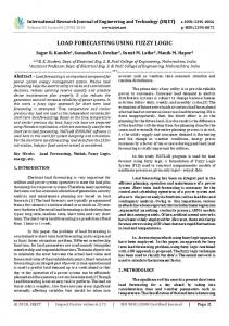
V. METHODOLOGY

Ttrain

Dtrain

Htrain

B. Data Preprocessing for Time Series Modeling For a time series alternating in time, a non-linear discretetime dynamic model for load forecasting is represented by: y (t + k ) = f ( y (t ), y (t + 1),..., y ((t + k ) − 1) ), k = 7

Kohonen Self-Organizing Map Historical load profile of two years used as training data

Ltrain

A. Feature Selection Features have been selected for use in the hybrid forecasting model to provide better prediction accuracy. Four features from the EUNITE competition dataset have been selected to evaluate the proposed forecasting model, which are as follows: • Maximum daily electricity load • Average daily temperature • Day type (weekday or weekend) • Annual holidays

SOM Training data clustered into two subsets: Lclust, Tclust, Dclust and Hclust

SVRs

ε-SVR-1 training with first data subset

Two cluster centers obtained from classified subsets

ε-SVR-2 training with first data subset

Subset 1 Subset 2

(5.1)

where y(t) is a vector representing the daily electricity load profile at time t = 0, 1, 2, ..., N, and k is the order of the dynamic system, which is a pre-determined time series shift constant. For the case of this experiment k = 7 is used in (5.1); i.e., historical load data of the first one week is used to calculate the load data of eighth day. Similarly, historical data from the second day until the eighth day (next 7 days) is used to calculate the load data of the ninth day, and so on, for the entire load data for the preceding two years. C. Architecture of Hybrid Network A hybrid artificial intelligence-based network is applied to reconstruct the dynamics of electricity load consumption using the time series of its observables. The proposed hybrid electricity forecasting model is shown in Figure 4, where the parameter subscripts: train, clust and test represent the training, clustered and testing data respectively. This model is based on a two stage architecture of the SOM and the epsilon-SVR. The hybrid electricity load forecasting model presented in this paper is developed, trained, and tested using MATLAB™ R2007b v7.5.0. The computer used was a Dell PowerEdge SC1420 Workstation with Windows XP, a 3.00 GHz Intel Xeon Processor and 512 MB of RAM. The Kohonen SOM model was implemented using the MATLAB Neural Network Toolbox and the epsilon-SVR models were implemented using the LIBSVM v2.85-1 Toolbox[6] for MATLAB. D. Data Representation Firstly, load and temperature time series data are linearly scaled (normalized) in the range from 0 to 1. Secondly, useful information is selected and a proper combination of features is selected to prepare the training dataset[3]. To represent calendar information, the day type feature uses seven binary digits [0, 1] to encode information for weekdays and weekends. The annual holidays feature uses one binary digit to encode information. To represent the historical electricity load for the preceding two years from January 1, 1997 to December 31, 1998, seven vector numerics for k = 7 in (5.1), from the preprocessed time series are used, each with a shift of one day. For temperature data only one numerical attribute is used from the normalized temperature data.

Decision based on Euclidean distance between cluster centers and testing data

d1 < d2

d2 < d1

ε-SVR-2 prediction ε-SVR-1 prediction Testing data

Ltest

Ttest

Dtest Htest

Predicted month-ahead electrical power load profile

Fig. 4. Proposed hybrid model for electricity load forecasting

E. Training and Testing Hybrid Network The training and testing for the hybrid electricity load forecasting model is outlined as follows: 1. In the first stage, the SOM clusters the space of the input training data set into two subsets with similar dynamical properties, in an unsupervised manner. The input variables for the SOM training are given in Table II. 2. Secondly, the SOM acts as a filtering scheme by generating two cluster centers from the clustered training dataset for each of the two subsets; based on individual location of each subset. 3. The three major parameters used in the SOM training are selected as follows: αi = 0.98, wp = 10exp(10) and e = 50, where αi is the initial learning rate, wp is the winning neuron criteria, and e is the number of epochs. 4. The incremental learning rate αf used in the Kohonen rule[2], is updated on each epoch iteration to calculate the winning neuron, using the expression:

α f (e) = α i ( −0.02e ) 5.

(5.2)

In the second stage, two ε-SVR (ε-SVR-1 and ε-SVR2) models are trained using the sequential minimal 54

6. 7.

optimization (SMO) algorithm individually, for each SOM clustered subset in a supervised manner. Next, two Euclidean distances between the cluster centers and the testing data are calculated; d1 and d2. Logical comparison of the Euclidean distances (d1 < d2) and (d2 < d1) as shown in Figure 4, provide the decision of selecting the appropriate ε-SVR model to fit the training data. The input variables for testing the two εSVR models are shown in Table III.

of error C, and kernel parameter γ, were selected to be 100 and 0.001 respectively. From the 10-fold cross-validation results obtained, the RBF kernel yielded the best accuracy, resulting in a MAPE of 1.73%. Hence, from this point onwards, all tests performed were done using the RBF kernel. TABLE IV PREDICTION ACCURACY BASED ON TYPE OF KERNEL Kernel type

TABLE II LIST OF INPUT DATA FOR SOM NETWORK TRAINING Input 1-7 8 9-15 16

8 9-15 16

MAPE 2.19%

Polynomial

C = 100, γ = 0.001, d = 2, r = 2

1.92%

Detail description

RBF

C = 100, γ = 0.001

1.73%

Load vector

Seven vector numerics of one week

Sigmoidal

C = 100, γ = 0.001, r = 0

2.33%

(Ltrain)

shifted load series from 97 to 98

Temperature

One vector numeric for average daily

(Ttrain)

temperature from 97 to 98

Day type

Seven binary digits representing

(Dtrain)

calendar information from 97 to 98

Holiday

One binary digit representing annual

(Htrain)

holidays from 97 to 98 TABLE III

1-7

Kernel parameters no values

Variable

LIST OF INPUT DATA FOR SVR-1 AND SVR-2 NETWORK SIMULATION Input

Linear

Variable

Detail description

Load vector

One vector for one week daily load

(Ltest)

from training data of 97 to 98

Temperature

One vector numeric for average daily

(Ttest)

temperature of January 99

Day type

Seven binary digits representing

(Dtest)

calendar information for January 99

Holiday

One binary digit representing annual

(Htest)

holidays for January 99

Cross-validation is used by dividing the training data into two sets: training set and validation set. The validation set uses different sets of one week historical data from the preceding two years data (from January 1, 1997 to December 31, 1998) to perform crossvalidation. 9. The best suited ε-SVR kernel, its parameters and optimal ε-SVR parameters: cost of error C, width of the ε-insensitive tube (loss function) ε, and the tolerance of termination criterion σ, are selected by generating 1 million random values for each parameter, and iterating them with different combinations to find the optimal set. 10. Finally, the month-ahead electricity load forecast for the 31 days of January 1999 is predicted using cross validation, and the MAPE is calculated.

TABLE V COMPARISON OF FORECASTING MODEL WITH OTHER TECHNIQUES Technique MAPE Forecasting model

SOM-SVR

1.42%

SVR

2.27%

ML-BPNN

3.31%

B. Parameter Optimization Through cross-validation trials, the best values for the εSVR parameters ε and σ were found to be 0.02 and 0.1 respectively. For finding the optimal values of C and the RBF kernel parameter γ, prediction accuracy of the hybrid electricity load forecasting model using different combinational values of the two parameters was determined. From the results obtained, two parameter values for ε-SVR1 and ε-SVR-2 were found, where C1 = 213.8381, γ1 = 0.0010, C2 = 52.8170 and γ2 = 0.0069 resulting in a MAPE of 1.42%.

8.

VI. EXPERIMENTAL RESULTS A. Kernel Selection The behavior of four different kernels namely: linear, polynomial, radial basis function (RBF) and sigmoidal for the ε-SVRs was observed using 10-fold cross-validation. Comparison of these kernels based on the accuracy of prediction of the forecasting model is shown in Figure 5. The parameter values selected for the kernels (defined in 4.3 4.4, 4.5 and 4.6) are shown in Table IV, where the cost

Fig. 5. Comparison of different kernels for ε-SVR model

C. Comparison of Forecasting Models For a comparative study, numerical simulations comparing with other load forecasting methods were also conducted. Besides using a hybrid SOM-SVR model, simulations using the EUNITE dataset were conducted for a stand-alone SVR and Multi-layer Back-propagation Neural Network (ML-BPNN) model, as shown in Figure 6. Overall results obtained, indicate that by far neural networks alone are not satisfactory as shown in Table V. The hybrid SOM-SVR model proved to be superior to the SVR and MLP-BPNN models, resulting in a MAPE of 55

1.42%. In addition, comparisons with previous work done on electricity load forecasting in [3] and [4], using the EUNITE competition[7] dataset revealed that, the proposed hybrid electricity load forecasting model has far better prediction accuracy than both of the forecasting models.

[6]

C.-C. Chang and C.-J. Lin. LIBSVM: A Library for Support Vector Machines. Available at: http://www.csie.ntu.edu.tw/~cjlin/libsvm

[7]

EUropean Network on Intelligent TEchnologies for Smart Adaptive Systems. Available at: http://www.eunite.org/. The competition page is: http://neuron.tuke.sk/competition/ Jawad Nagi was born in Karachi, Pakistan on March 23, 1985. He received his Bachelors degree from Universiti Tenaga Nasional (UNITEN), Malaysia with honors in Electrical and Electronics Engineering in 2007. He is currently working as a Project Engineer in the Power Engineering Centre at Universiti Tenaga Nasional, working towards his Masters degree in Electrical Engineering. His research interests include pattern recognition, image processing, fuzzy logic, neural networks and

support vector machines. Keem Siah Yap received his Bachelors and Masters degree both from Universiti Teknologi Malaysia (UTM) in 1998 and 2000 respectively. Currently he is working towards his Ph.D. degree in Electronic Engineering from Universiti Sains Malaysia (USM). He is currently a Senior Lecturer in the Department of Electronic and Communication Engineering, Universiti Tenaga Nasional (UNITEN), Malaysia. His research interests include neural networks, fuzzy logic, pattern

Fig. 6. Comparison of different forecasting models

VII. CONCLUSION In this paper, a novel technique for mid-term electricity load forecasting has been presented based on a hybrid SOM-SVR model. Experimental results obtained demonstrate the feasibility of successfully applying this new hybrid model for electricity load forecasting. The proposed model has three notable advantages. Firstly, it has the ability to tackle with the non-stationarity in the electricity load time series. Secondly, it can treat regular days (weekdays and weekends) and annual holidays with different schemes. Lastly, it has strong robustness and can be easily modified for different power systems. In addition, the structural risk minimization principle in SVRs proved to be superior compared to the empirical risk minimization principle employed by conventional ANNs. Comparisons with the previous winner[3] of the EUNITE competition[7], and [4] shows that this hybrid electricity load forecasting model has far better prediction accuracy compared to its predecessors. REFERENCES [1]

S. Fan and L. Chen, “Short-Term Load Forecasting based on Adaptive Hybrid Method”, IEEE Transactions on Power Systems, Vol. 21, No. 1, Feb. 2006, pp. 392-401.

[2]

J. Nagi, S. Khaleel Ahmed and F. Nagi, “A MATLAB based Face

recognition and robotics. Sieh Kiong Tiong obtained his Bachelors and Masters degrees from Universiti Kebangsaan Malaysia (UKM), in Electrical, Electronic and System Engineering in 1997 and 2000 respectively, and Ph.D. degree from Universiti Kebangsaan Malaysia (UKM), in Mobile Communication in 2006. He is currently a member of the Power Engineering Centre of Universiti Tenaga Nasional (UNITEN). He is working in the Electronic and Communication Engineering Department of Universiti Tenaga Nasional as a Senior Lecturer. His research interests include digital electronics, microprocessor systems, artificial intelligence and mobile cellular systems. Syed Khaleel Ahmed received his Bachelors degree from Anna University, India in Electrical and Electronics Engineering in 1988, and Masters degree in Electrical and Computer Engineering from the University of Massachusetts Amherst, United States in 1994. He is currently working in the Electronic and Communication Engineering Department of Universiti Tenaga Nasional (UNITEN) as a Senior Lecturer. His research interests include robust control, fuzzy logic and control, neural networks, robotics, signal processing and numerical analysis.

Recognition System using Image Processing and Neural Networks” in Proc. of The 4th International Colloquium on Signal Processing and its Applications”, CSPA 2008, March 2008, pp. 83-88. [3]

B.-J. Chen, M.-W. Chang, and C.-J. Lin, “Load Forecasting using Support Vector Machines: A Study on EUNITE Competition 2001”, IEEE Transactions on Power Systems, Vol. 19, No. 4, Nov. 2004, pp. 1821-1830.

[4]

S. Rahat Abbas and M. Arif, “Electric Load Forecasting using Support Vector Machines Optimized by Genetic Algorithm”, in Proc. of Multitopic Conference, INMIC 2006, Dec. 2006, pp. 395-399.

[5]

W.-C. Hong, P.-F. Pai, C.-T. Chen, and C.-S. Lin, “Support Vector Machines with Simulated Annealing Algorithms in Electricity Load Forecasting”, Energy Conversion and Management, Vol. 46, No. 17, Oct. 2005, pp. 2669-2688.

56