A Deployable Electrical Load Forecasting Solution for ...

A Deployable Electrical Load Forecasting Solution for Commercial Buildings Naveen Kumar Thokala

Aakanksha Bapna

M. Girish Chandra

TCS Research and Innovation Bangalore, India Email: [email protected]

TCS Research and Innovation Bangalore, India Email: [email protected]

TCS Research and Innovation Bangalore, India Email: [email protected]

Abstract—Electrical load forecasting for buildings plays a key role in the smart-grid paradigm, since accurate forecasts help in efficient energy management by addressing peak-load shaving, load scheduling and effective demand response programs. This paper presents a practical solution, which can be readily deployed, by considering various real-life issues. Load forecasting algorithms are developed using Non-linear AutoRegressive model with eXogenous input (NARX) neural network and Support Vector Regression (SVR) to forecast the power consumption for day ahead, week ahead and month ahead at 15 minute granularity. Missing values, outliers in the power consumption data are treated using simple but effective techniques based on the thorough understanding of the power consumption time-series data. Autoregressive features, temperature and some efficacious contextual information, which are completely pertinent to this problem, are being derived to model this heterogeneous time series that consists of disparate patterns on weekdays, weekends and holidays. The novelty of the solution lies in the fact that it extensively models all the variations and produces accurate long term predictions at high granularity (15 min). The algorithms are validated using the actual power consumption data from three Office buildings; forecasting accuracy of both SVR and NARX neural network are comparable, the latter performs better by a thin margin. The average forecasting accuracy is nearly 93%, 8890% and 85-87% for day ahead, week ahead and month ahead forecasting respectively. Keywords - load forecasting, NARX neural networks, support vector regression, energy management.

I. I NTRODUCTION Forecasting electrical load for commercial buildings amounts to estimating the future values of power consumption for the horizons of interest at different levels of granularity. The total power consumption in a building depends on all the loads operating in it. Major loads like Heating, Ventilation and Cooling (HVAC), Lighting and Computing which constitute almost 80% [1] of the total power consumption in a building, and are in turn influenced by factors like temperature, humidity, behavioral pattern of the occupants, holidays etc. These factors are highly varying, which in turn causes the variation in the total power consumption making the forecasting problem very challenging. Accurate prediction of the power consumption is helpful in prudent energy management as it can facilitate the building manager to carry out the following : •

Bidding Power : Which helps in optimizing the cost incurred in buying electricity from the utility

•

•

•

Peak Load Shaving : With high resolution load forecasting ( i.e. predicting power consumed in every 15/30 minute) the exact intervals when the peak load occurs can be known that can assist the building manager to schedule the loads judiciously, Addressing Demand Response : High and low power consuming loads can be scheduled appropriately to reduce the power consumption during the peak-pricing periods resulting in gaining financial incentives from the utility. Deviations in Building’s Power Consumption : The load forecasting model can be used to identify the deviations in building power consumption i.e. large discrepancies between the predicted and actual power consumption pattern under similar conditions would be alerted to the building manager.

This motivates us to solve the problem of electrical load forecasting for a commercial building. The building energy systems are mostly modeled using the available information like historical power consumption data from smart meters and temperature. However, such complex data cannot be modeled using only these two parameters. Additional features are derived and contextual information is also used in order to capture the dynamics of the system which are not explicit. There are many load forecasting solutions in literature which focus mainly on Utilities ([2],[3],[4]), like sub-stations load forecasting is addressed in the work by Luiz et. al. [4], which uses Transfer Function model and forecasts week ahead hourly load consumptions using exogenous variables like temperature, humidity and wind speed. Some of the earlier works related to building load forecasting can be traced in ([5],[7],[10],[11],[12]). A good study of models for forecasting loads for air-conditioned non-residential buildings is described in [5]. Ivan et. al. performed day ahead load forecasting for four such buildings and compared the performance of different models like Artificial Neural Network (ANN), Support Vector Machines (SVM), Polynomial and AutoRegressive Integrated Moving Average (ARIMA); reported ARIMA as the best model. In many recent works, ANNs have been used to predict long and short-term loads for non-residential buildings as mentioned in ([7],[6],[8],[9]). In [10], Cevik et. al. proposed a Fuzzy logic based method to model power consumption

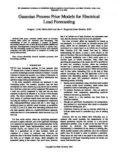
on holidays. They have analyzed the patterns observed in power consumption on national holidays, religious holidays and days around holidays. Their work corroborates our notion that power consumption is dependent on occupants’ behavior which is different on weekdays, weekends and holidays. Fux et. al.[11] also modeled weekdays, weekends and holidays separately and did short-term forecast of power values for a large office building. They compared the performance of ANN and SVR with least squares and reported that the latter performed better. There exist very few attempts in the space of high resolution forecasting. Yoon et. al. [12] used pattern ratio based method for short-term load forecasting at 15 minutes granularity and they assumed that the difference between any two consecutive power consumption values will be very small. This method requires very less data to predict next values which makes it very fast but accuracies were compromised. In our work, we attempted to develop a deployable solution for load forecasting by robust modeling of the building’s energy consumption; different variations due to holidays, weekends, optional holidays etc. are absorbed in to the model in the form of features. Three separate models are developed to perform high resolution load forecasting for different time horizons (day ahead, week ahead and month ahead) and to the best of our knowledge, this is the first attempt to address high resolution load forecasting i.e. at 15 minutes granularity for long time horizon (month ahead prediction). The block diagram as shown in Figure 1, depicts the energy management system, the solution includes preprocessing stage where the raw data churning out from the smart-meter is refined using the novel approaches which is followed by feature extraction stage. Thereafter, relevant subset of these features is employed to train different models for different time horizons. The forecasting models are overhauled after some definite time intervals to accommodate the changes in power consumption resulting from various factors like degradation, aging of the building etc. The inference engine acts on the load forecasting results to facilitate building manager or automatic control system to take necessary actions towards prudent energy management as depicted in the block diagram. The major contributions of this paper are • •

•

Novel methods to preprocess the data to deal with outliers/erroneous data and missing data. Efficient algorithms for high resolution forecasting for different time horizons: day ahead, week ahead and month ahead. A single robust system that models the power consumption data; the time series of data comprises of disparate patterns on weekdays, weekends, holidays etc. all of which get absorbed into one model.

The organization of the paper is as follows. Data preprocessing and feature extraction steps are detailed in Section II. The load forecasting algorithms are explained in Section III. Results for time horizons considered are shown in Section IV and there is a discussion on the results in Section V and

Fig. 1. Block Diagram for Building Energy Management

conclusions are presented in the Section VI. II. DATA P RE - PROCESSING AND F EATURE E XTRACTION While developing the models for forecasting, we considered the data captured well beyond the present instant under consideration. Effectively we have sufficient amount of historical power consumption data at 15 minutes granularity for around eight months. Also considered is the temperature data at 1 hour granularity for the same duration. A. Missing Values and Outliers in Power Data The power data is erroneous at places due to factors like malfunctioning of smart meter, communication failure or the failure of the meter itself. These factors introduce discrepancies in the data in the form of missing values or outliers. Missing values if very few, can be estimated using interpolation but if the values are missing continuously for a day or longer, it requires appropriate methods of estimation to address these bursts. Detecting outliers is very challenging due to many reasons like (i) it is not possible to define a fixed threshold based on standard deviation, as the dynamic range of power data is varying for different buildings (ii) the underlying system generating the power consumption data (P ) is not time-invariant, i.e. P is not same for identical temperature for different days and at different times of the day implying that power consumption has explicit dependency on time apart from temperature. To address this, a hierarchical approach is proposed where first the power consumption data is separated into two series, i.e. for weekdays and weekends and then, the power consumption at each time instant t, for all the days in the data set is considered as one time series. Since these time series represent power consumption values at the same time instant for all the days, the variance of the series would be very low and most of the values should be close to mean. In this case, the values beyond twice the standard deviation

from the mean are considered as outliers. Outlier are identified using the following: O(i, t) = 1 if P (i, t) > |PM ean (t) ± (2 ∗ PSD (t))| = 0 otherwise. where P (i, t) represents the power consumption on ith day at tth time instant, O(i, t) is a binary variable which is true if P (i, t) is an outlier. PM ean (t) is the mean of the time series at time t for all the days and PSD (t) is the standard deviation of the time series and P (i, t) is the power consumption value on ith day at time instant t. The outliers are replaced using weighted moving average filter, where the recent values in the series are given more weight than the farther values. P (k, t) = w1∗P (k −1, t)+w2∗P (k −2, t)+w3∗P (k −3, t) (1) where, w1, w2, w3 are weights in the decreasing order, P (k, t) is the estimation of power for outliers at time instant t on k th day. P (k − 1, t) is the power consumption value at same time instant on previous day. There are some time instants where consumption values are not available (i.e. missing values). If the values are very few in number (less than 4), linear interpolation is used to fill in those values as the power consumption would not have varied much in one hour time period. But, if there are more values missing continuously, then missing values are estimated using the weighted moving average filter approach as given in equation 1. B. Feature Extraction Towards time series analysis of power consumption data, it is required to derive relevant and appropriate features to train the algorithms effectively and generate accurate predictions. The following features are used in our work: 1) Temperature: Forecasting at different time horizons ahead of time necessitates having the temperature information as well for that horizon ; if the time horizon is a day or a week, hourly temperature can be obtained from online weather source [13] and interpolated for 15 minutes in order to synchronize with the power consumption data. But, if the time horizon is a month, it is observed that only minimum and maximum temperature forecasts are made available. To address this problem for high resolution forecasting month ahead, it requires to estimate the hourly temperature from the available information like min-max values. Therefore, we used method 1 specified in [14] by D.C. Reicosky et. al. for the hourly temperature estimation. 2) Autoregressive Features: Autoregressive features are derived from historical power consumption values using different lags. These lags are identified using the autocorrelation function. It was discovered that data points at day lag and week lag have a very good correlation with the current data point. Moreover, the correlation

is high for week lag compared to day lag. As the power consumption data considered is from large office buildings, has a specific pattern which is dependent on time and day of the week, i.e. this week Tuesday’s power consumption is very similar to previous week Tuesday’s power consumption and so on for the power consumption of different days in the same week. Upon careful inspection and experimentation, different lags which would be relevant for different prediction horizons were chosen. • For day ahead, the previous day’s, and previous three weeks same day power consumption information is used, as these features have more impact on the day ahead prediction. • For week ahead, previous three weeks’ same days’ power consumption are used as features as these are sufficient and most recent useful information is made available to model the week ahead forecasting. • For month ahead, previous fifth to eighth weeks’ same days’ power consumption are used as features, as these are sufficient and most recent useful information available to model the month ahead forecasting. 3) Contextual Information: Contextual information like weekday/weekend, day of the week, time of the day, holidays, optional holidays etc., are also used as the features. Weekends definitely observe a very low power consumptions w.r.t. weekdays in office building. Holidays are different from weekends (Saturday/Sunday) because these have an impact on power consumption on the days before and after holidays, as people tend to take long leaves if the holiday is close to weekend, affecting the power consumption pattern in their neighbourhood. Optional holidays are different from holidays, and it is generally given on religious festivals, so not everyone will avail that resulting in only partial reduction in the number of occupants in the building and affecting the power consumption. This information majorly contributes to learning a single resilient model to represent the power consumption data and to provide some veracious information for long term prediction. The aforementioned features like temperature, contextual information (time of the day, day of the week, weekend/weekday), and autoregressive terms of power consumption are encapsulated in feature vector (X) as input to the forecasting algorithms: X = {T (t), P1W (t), .., P8W (t), T oD, DoW, H}

(2)

where, T (t) represents the external temperature at time t, P1W (t), .., P8W (t) represents the power consumption lags (auto-regressive terms), T oD, DoW and H represents the contextual information like time of the day, day of the week, and holiday respectively. The subset of these features are used to train the models depending on the forecasting time horizon.

III. L OAD F ORECASTING A LGORITHMS A. NARX Neural Networks Non-linear autoregressive neural network with exogenous input (NARX NN) is known for its application for chaotic time series analysis generated by dynamical systems.([15],[17]). This model is a partial recurrent neural network (RNN) as the memory is embedded in to the network by adding autoregressive terms as inputs apart from the exogenous variables. These features will help in capturing the long-term dynamics of the time series and contextual information like time of the day, day of the week and other features will help in capturing the short-term dynamics of the system. In [16], NARX neural network is used to forecast day ahead power consumption for the buildings; only limited results were presented in that article. In the current work, it is enhanced and made robust to handle high resolution forecasting for different time horizons like day ahead, week ahead and month ahead. Three different functions are learned for three time horizons using NARX neural network and these functions are used to forecast the power consumption for the respective time horizon. The function for load forecasting using NARX neural network is given as follows: P (i, t) = fN ARX (X),

(3)

where fN ARX is the function learnt using NARX neural network, X is feature vector chosen appropriately for different time horizons and P (i, t) is the power predicted for day i at time step t. B. Support Vector Regression While performing Support Vector Regression (SVR), the data is transformed into higher dimensional space F using non-linear mapping φ and linear regression is performed in this space [18]. f (x) = (φ(x) ∗ w) + b

(4)

Thus, linear regression in the higher dimensional space F corresponds to non-linear regression in the low dimensional space (Rn ) and where w represents the weights in F space and b is the threshold. The ability to choose a sub-set of points (called support vectors) to build the model makes it computationally fast and very efficient in predicting highly complex time series accurately [19]. The load forecasting model developed using SVR is as shown in the following: P (i, t) = fSV R (X),

(5)

models are developed using almost eight months of power consumption and temperature data from three office sites (A, B, C) from three different cities in India. Among the three buildings, compared to the behaviour of A and B , the building C has some unpredictable pattern, as can be seen from the Figure 3. The NARX neural network used has one hidden layer with 15 neurons. The SVR-based load forecasting algorithm was tuned for the cost of constraints violation = 1 and tolerance for termination criterion = 0.01 using Radial Basis Function (RBF) kernel for learning the function for forecasting. We compared the forecasts generated by our algorithms with the standarad forecasting algorithms ARIMA and Linear Regression (LR) for day ahead forecasts and with only Linear Regression for week and month ahead forecasts. The ARIMA models start predicting the mean value associated with trend of the time series i.e a straight line for long horizon forecasts as auto-regressive terms converge to mean of the time series. Hence, ARIMA models can not be used for week and month ahead forecasts. In summary, ARIMA models are suitable for only short-term forecasts, and not for long-term forecasts. Towards benchmarking our results against the LR (rudimentary but popular) and ARIMA models, the same features are used for all the cases. For comprehensive evaluation of the performance of the algorithms, we examined two error metrics: Mean Absolute Percentage Error (MAPE) and Normalized Root Mean Square Error (NRMSE). MAPE is a very popular error metric used to measure the performance of the forecasting algorithms and NRMSE facilitates the comparison between datasets or models with different scales. It indicates the residual variance of the predictions. Note: All errors stated in the tables I, II and III are the average errors computed by taking mean of the errors obtained for multiple such predictions made for different time windows. A. Day Ahead Forecast Day ahead forecasting involves forecasting building power consumption for the next 96 time steps. The accuracy of day ahead forecasting is very high, almost 93% on an average, with the latest information is available to the algorithm in the form of previous day and previous weeks same day power consumption. Figures 2 and 3 show the forecasting performance of the algorithms for the buildings A and C. The errors incurred while forecasting day ahead for the three buildings considered are as shown in the Table I.

where fSV R is the function learnt using SVR, X is feature vector chosen appropriately for different time horizons and P (i, t) is the power predicted for day i at time step t. IV. R ESULTS A prototype of the proposed solution is developed using R package to validate its capability in forecasting the power consumption at 15 minutes granularity for different time horizons like day ahead, week ahead and month ahead. The

Fig. 2. Day Ahead Forecast for Building A

TABLE II W EEK A HEAD F ORECASTING E RRORS : E1 (MAPE), E2 (NRMSE) Algorithm

Building A

Building B

Building C

NARX NN SVR LR

E1 12 9.1 14

E1 9 9.1 12

E1 11 10 15.8

E2 0.11 0.10 0.18

E2 0.12 0.11 0.16

E2 0.10 0.10 0.19

Fig. 3. Day Ahead Forecast for Building C

TABLE I DAY A HEAD F ORECASTING E RRORS : E1 (MAPE), E2 (NRMSE)

are as shown in the Figures 4 and 5. The forecasting errors for week ahead for the three buildings considered are as shown in Table II.

Algorithm

Building A

Building B

Building C

C. Month Ahead Forecast

NARX NN SVR ARIMA LR

E1 9 8 22 12

E1 8 7 24 11

E1 9 8 27 13

High resolution month ahead forecasting i.e at 15 minutes granularity is very challenging due to the reasons mentioned in Section IV-B. All these arguments are valid and much more complex in the case of month ahead forecasting. Inspite of this, long time horizon forecasting at high resolution is worked out effectively, since the non-explicit dynamics of the system is captured to a large extent using contextual information. Reasonably good accuracy is achieved for month ahead forecasting also, as it is evident from Figures 6 and 7. The forecasting errors for month ahead for the three buildings considered are as shown in the Table III.

E2 0.12 0.13 0.24 0.19

E2 0.09 0.13 0.28 0.14

E2 0.12 0.13 0.29 0.15

B. Week Ahead Forecast Week ahead forecasting involves forecasting power consumption for the next week days at 15 minutes granularity. The forecasting accuracies for week ahead are less than day ahead by small percentage because (i) temperature forecast error would be more as the time horizon increases and (ii) capturing dynamics of the system which are not explicit is difficult as the time horizon increases, which are accounted by default when latest power data is considered in the case of day ahead forecasting.

Fig. 6. Month Ahead Forecast for Building A

Fig. 4. Week Ahead Forecast for Building A

Fig. 7. Month Ahead Forecast for Building C

TABLE III M ONTH A HEAD F ORECASTING E RRORS : E1 (MAPE), E2 (NRMSE) Fig. 5. Week Ahead Forecast for Building C

Algorithm

Building A

Building B

Building C

By considering contextual information like weekday, holidays, weekend etc., some information can be gleaned about the non-explicit dynamics to improve the week-ahead forecast. The performance of the algorithms for week ahead forecasting

NARX NN SVR LR

E1 13 12 16.3

E1 11 9.8 15.2

E1 15 14 17.4

E2 0.12 0.11 0.19

E2 0.13 0.11 0.17

E2 0.13 0.12 0.19

V. D ISCUSSION A. Performace Comparison From Figures and Tables in the results Section IV, it is evident that the proposed algorithms are lot more efficient than ARIMA and LR. Among the proposed two, SVR-based one is performing better than NARX neural network by a small margin for all the buildings and time horizons. One possible reason can be, unlike NARX neural network, SVR learning involves two stages of learning, where the initial non-linear mapping is followed by linear processing on support vectors. It gives a better handle to solve the problem of forecasting through the said regression. This two staged approach makes SVR more accurate and thus even the time series generated from complex dynamics like building energy systems can be modeled precisely using SVR . B. Incremental Model Update The forecasting algorithms are overhauled after definite time intervals to address the changes that take place in the building for maintaining the accuracy. The major changes include •

•

Different equipments used in the building like HVAC systems (air handling units, ducts, etc.), lighting, computing etc would be efficient during the early life and degrade with time, causing performance degradation of the energy systems and There can be increase or decrease in power consumption due to some major changes in the building like change in number of occupants, replacing old equipment with new equipment etc.

These might cause a large difference between the forecast and the actual power consumption resulting in large errors. Whenever this deviation goes beyond some threshold, the parameters of the forecasting algorithms are updated using the latest power consumption data for all the three horizons to improve the forecasting accuracy. VI. C ONCLUSION A holistic solution for forecasting the Office Buildings energy for different time horizons at a high granurality has been worked out, by addressing: (i) effective handling of the outliers/missing values and (ii) incorporation of pertinent features and contextual information to capture the underlying dynamics. The models are trained on the actual data from the smart meters of the real buildings and are tested for different time horizons. We have been able to construct models based on SVR and NARX, which can solitarily capture the heterogeneous behaviour of the power consumption time series because of different patterns on weekdays, weekend and holidays, all of which have been picked up elegantly. The performance results on the actual buildings demonstrated their efficacy, pointing to the usefulness of the proposed solution in Energy Management.

R EFERENCES [1] Kwatra, Sameer, Jennifer Thorne Amann, and Harvey M. Sachs. ”Miscellaneous energy loads in buildings.” American Council for an EnergyEfficient Economy, 2013. [2] Swaroop, R., and A. Abdulqader Hussein. ”Load Forecasting For Power System Planning And Operation Using Artificial Neural Network At Al Batinah Region Oman.” Journal of Engineering Science and Technology 7.4 (2012): 498-504. [3] Eisa Almeshaiei, Hassan Soltan, ”A methodology for Electric Power Load Forecasting”. Alexandria Engineering Journal, Volume 50, Issue 2, June 2011, Pages 137-144. [4] Friedrich, Luiz, and Afshin Afshari. ”Short-term forecasting of the Abu Dhabi electricity load using multiple weather variables.” Energy Procedia 75 (2015): 3014-3026. [5] Fernndez, Ivn, Cruz E. Borges, and Yoseba K. Penya. ”Efficient building load forecasting.” Emerging Technologies and Factory Automation (ETFA), 2011 IEEE 16th Conference on. IEEE, 2011. [6] W. Mai, C. Y. Chung, T. Wu and H. Huang, ”Electric load forecasting for large office building based on radial basis function neural network,” 2014 IEEE PES General Meeting — Conference and Exposition, National Harbor, MD, 2014, pp. 1-5. [7] Bunnoon, Pituk. ”Mid-Term Load Forecasting Based on Neural NetworkAlgorithm: a Comparison of Models.” International Journal of Computer and Electrical Engineering 3.4 (2011): 600. [8] Kaur, Navjot, and Er Amrit Kaur. ”Electricity demand prediction using artificial neural networks in data mining.” International Journal For Technological Research In Engineering Volume 2, Issue 8, April-2015 [9] Chae, Young Tae, et al. ”Artificial neural network model for forecasting sub-hourly electricity usage in commercial buildings.” Energy and Buildings 111 (2016): 184-194. [10] Cevik, Hasan H., and Mehmet unkas. ”A Fuzzy Logic Based Short Term Load Forecast for the Holidays.” International Journal of Machine Learning and Computing 6.1 (2016): 57. [11] Fux, Samuel Felix, et al. ”Short-term thermal and electric load forecasting in buildings.” CISBAT (International Conference on Clean-tech for Smart Cities and Buildings: From Nano to Urban Scale). No. EPFLCONF-211899. 2013. [12] Yoon, Ah-Yun, Hyeon-Jin Moon, and Seung-Il Moon. ”Very shortterm load forecasting based on a pattern ratio in an office building.” International Journal of Smart Grid and Clean Energy, vol. 5, no. 2, April 2016: pp. 94-99 [13] ’Accuweather Weather Forecast’, http://www.accuweather.com/en/in/indiaweather. [14] Reicosky, D. C., et al. ”Accuracy of hourly air temperatures calculated from daily minima and maxima.” Agricultural and Forest Meteorology 46.3 (1989): 193-209. [15] Eugen Diaconescu. 2008. “The use of NARX neural networks to predict chaotic time series.” WSEAS Trans. Comp. Res. 3, 3 (March 2008), 182191. [16] Naveen Kumar Thokala and M. Girish Chandra. 2016. Disaggregated Forecasting for Large Office Buildings: Poster Abstract. In Proceedings of the 3rd ACM International Conference on Systems for Energy-Efficient Built Environments (BuildSys ’16). ACM, New York, NY, USA, 231-232 [17] Chuanjin Jiang and Fugen Song, ”Forecasting chaotic time series of exchange rate based on nonlinear autoregressive model,” 2010 2nd International Conference on Advanced Computer Control, Shenyang, 2010, pp. 238-241. [18] Mller, K-R., et al. ”Predicting time series with support vector machines.” International Conference on Artificial Neural Networks. Springer Berlin Heidelberg, 1997. [19] Mukherjee, Sayan, Edgar Osuna, and Federico Girosi. ”Nonlinear prediction of chaotic time series using support vector machines.” Neural Networks for Signal Processing [1997] VII. Proceedings of the 1997 IEEE Workshop. IEEE, 1997.